Raleigh, NC North Carolina State University Department of … · A. A. Markov Anniversary Meeting...
72
Updating Markov Chains Carl Meyer Amy Langville Department of Mathematics North Carolina State University Raleigh, NC A. A. Markov Anniversary Meeting June 13, 2006
Transcript of Raleigh, NC North Carolina State University Department of … · A. A. Markov Anniversary Meeting...

UpdatingMarkovChains
Carl MeyerAmy Langville
Department of MathematicsNorth Carolina State UniversityRaleigh, NC
A. A. Markov Anniversary Meeting
June 13, 2006
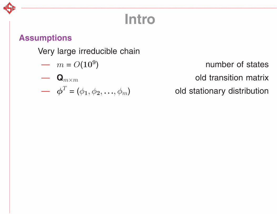
IntroAssumptions
Very large irreducible chain
— m = O(109) number of states
— Qm×m old transition matrix
— φT = (φ1, φ2, . . ., φm) old stationary distribution
IntroAssumptions
Very large irreducible chain
— m = O(109) number of states
— Qm×m old transition matrix
— φT = (φ1, φ2, . . ., φm) old stationary distribution
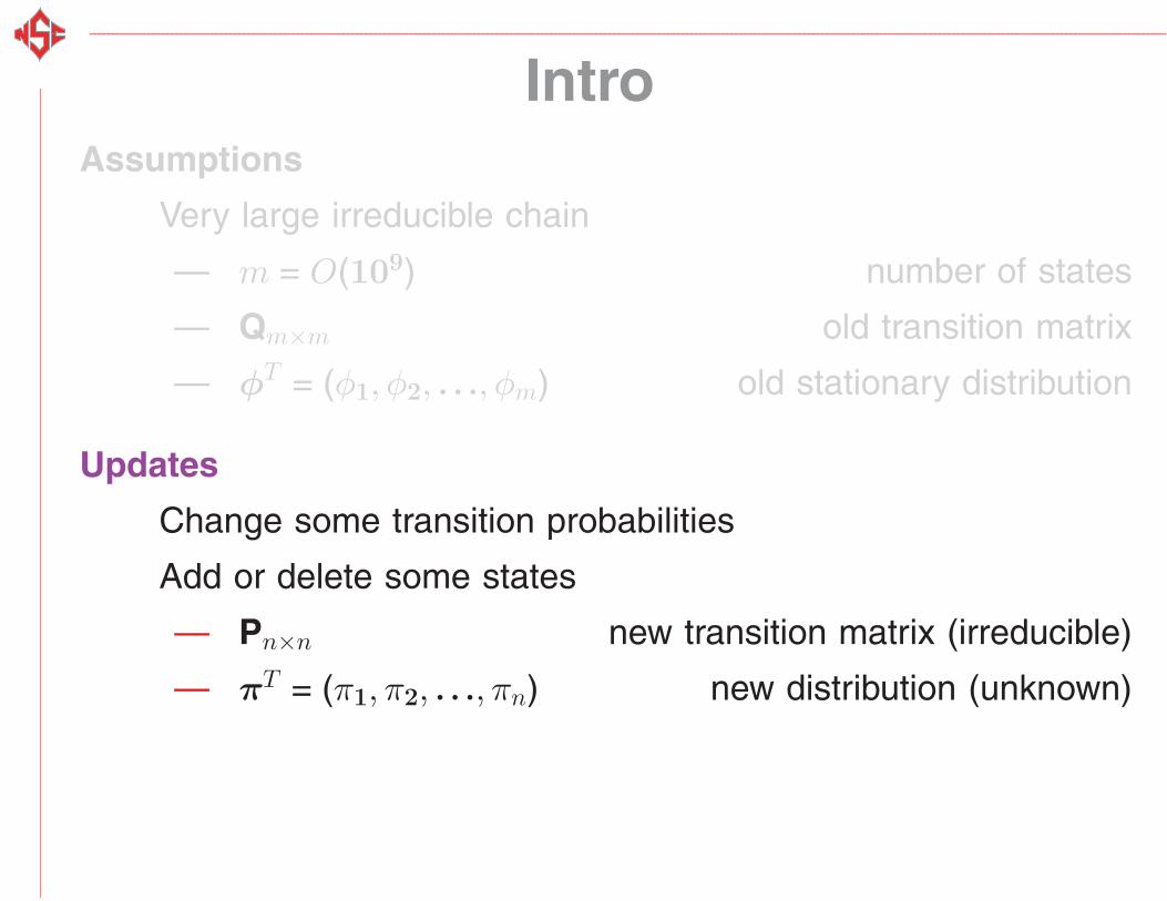
Updates
Change some transition probabilities
Add or delete some states
— Pn×n new transition matrix (irreducible)
— πT = (π1, π2, . . ., πn) new distribution (unknown)
IntroAssumptions
Very large irreducible chain
— m = O(109) number of states
— Qm×m old transition matrix
— φT = (φ1, φ2, . . ., φm) old stationary distribution
Updates
Change some transition probabilities
Add or delete some states
— Pn×n new transition matrix (irreducible)
— πT = (π1, π2, . . ., πn) new distribution (unknown)
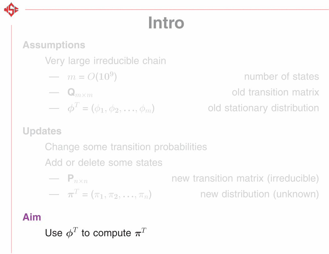
Aim
Use φT to compute πT
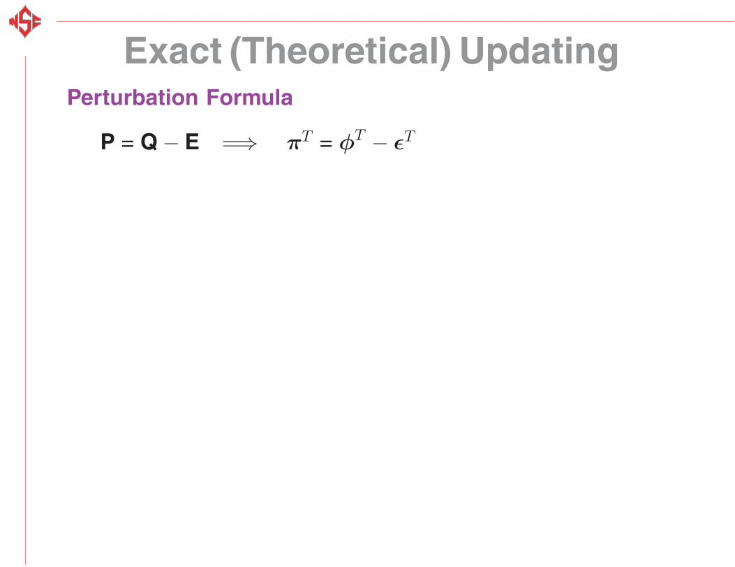
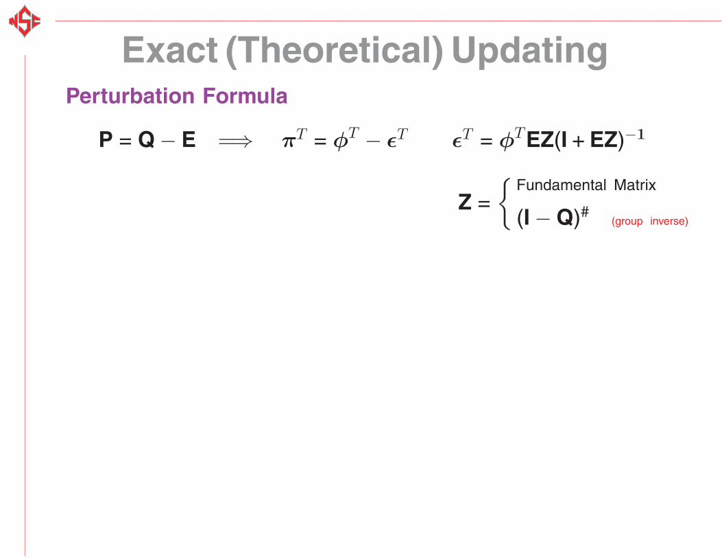
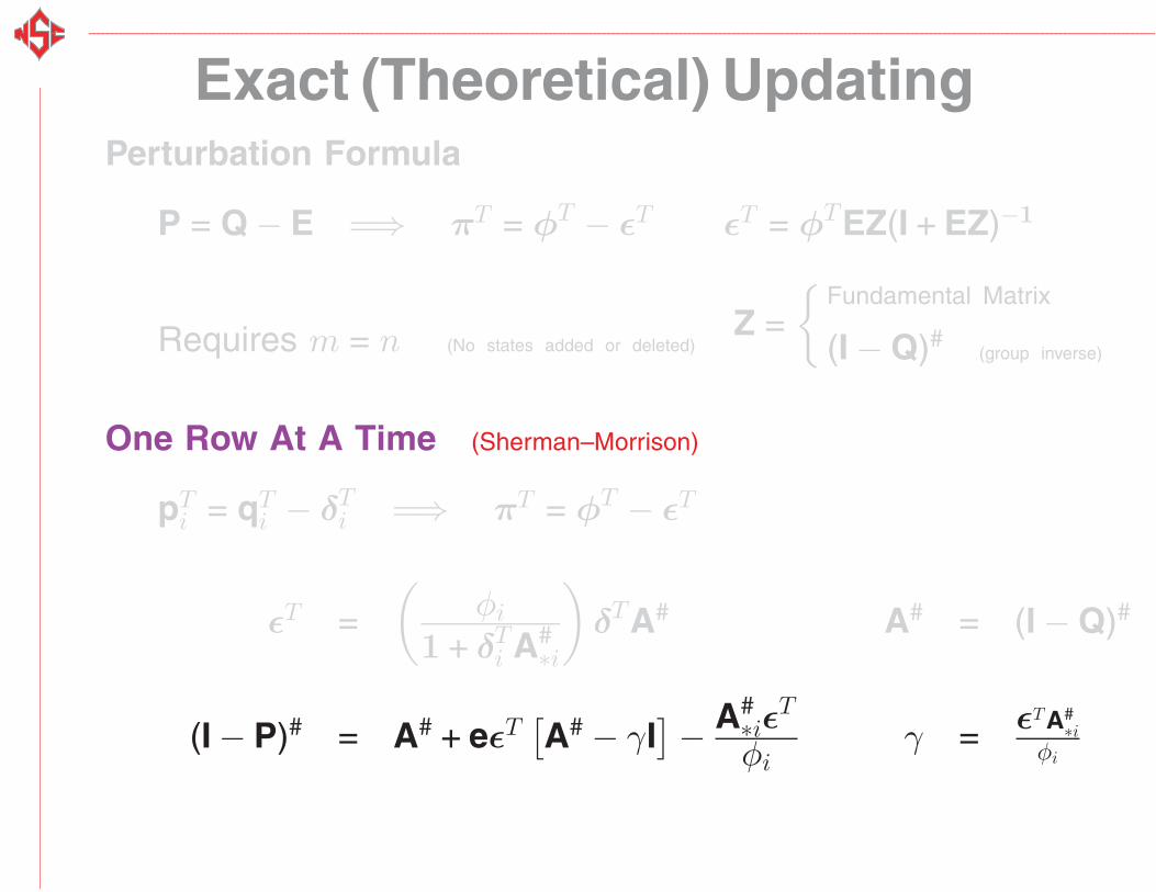
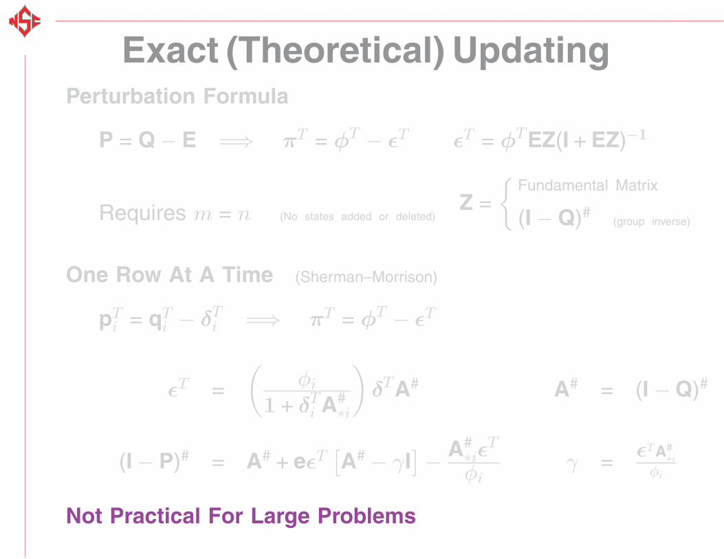
Exact (Theoretical) UpdatingPerturbation Formula
P = Q − E =⇒ πT = φT − εT
Exact (Theoretical) UpdatingPerturbation Formula
P = Q − E =⇒ πT = φT − εT εT = φTEZ(I + EZ)−1
Z ={
Fundamental Matrix
(I − Q)#(group inverse)
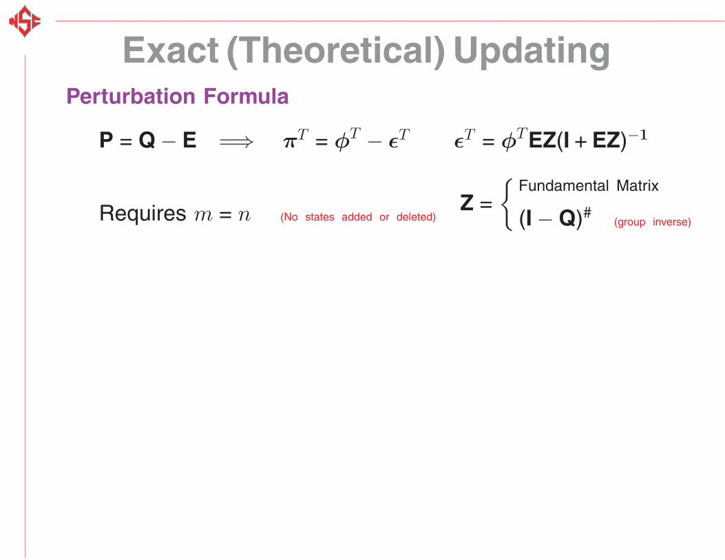
Exact (Theoretical) UpdatingPerturbation Formula
P = Q − E =⇒ πT = φT − εT εT = φTEZ(I + EZ)−1
Z ={
Fundamental Matrix
(I − Q)#(group inverse)Requires m = n (No states added or deleted)
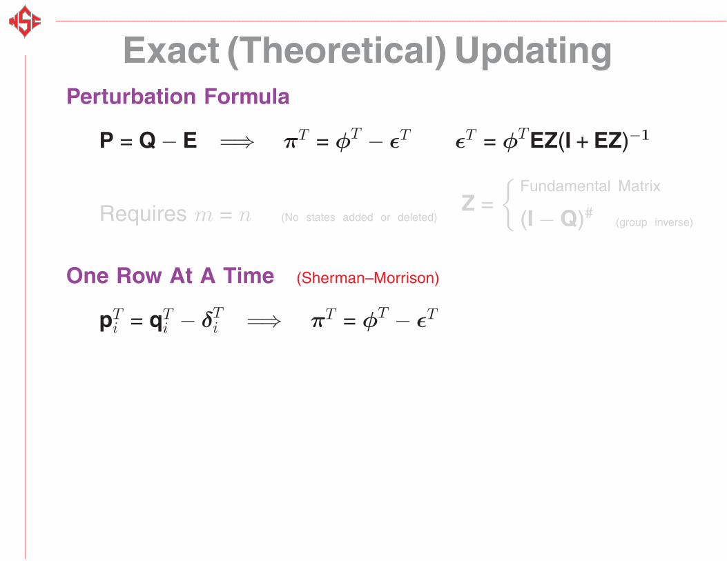
Exact (Theoretical) UpdatingPerturbation Formula
P = Q − E =⇒ πT = φT − εT εT = φTEZ(I + EZ)−1
Z ={
Fundamental Matrix
(I − Q)#(group inverse)Requires m = n (No states added or deleted)
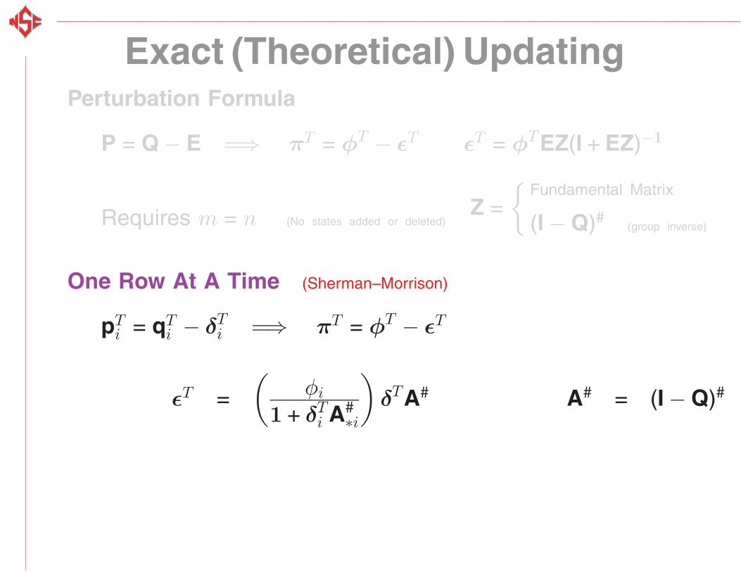
One Row At A Time (Sherman–Morrison)
pTi = qT
i − δTi =⇒ πT = φT − εT
Exact (Theoretical) UpdatingPerturbation Formula
P = Q − E =⇒ πT = φT − εT εT = φTEZ(I + EZ)−1
Z ={
Fundamental Matrix
(I − Q)#(group inverse)Requires m = n (No states added or deleted)
One Row At A Time (Sherman–Morrison)
pTi = qT
i − δTi =⇒ πT = φT − εT
εT =(
φi
1 + δTi A#
∗i
)δTA# A# = (I − Q)#
Exact (Theoretical) UpdatingPerturbation Formula
P = Q − E =⇒ πT = φT − εT εT = φTEZ(I + EZ)−1
Z ={
Fundamental Matrix
(I − Q)#(group inverse)Requires m = n (No states added or deleted)
One Row At A Time (Sherman–Morrison)
pTi = qT
i − δTi =⇒ πT = φT − εT
εT =(
φi
1 + δTi A#
∗i
)δTA# A# = (I − Q)#
(I − P)# = A# + eεT[A# − γI
]− A#
∗iεT
φiγ = εTA#
∗iφi
Not Practical For Large Problems
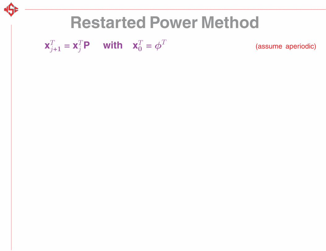
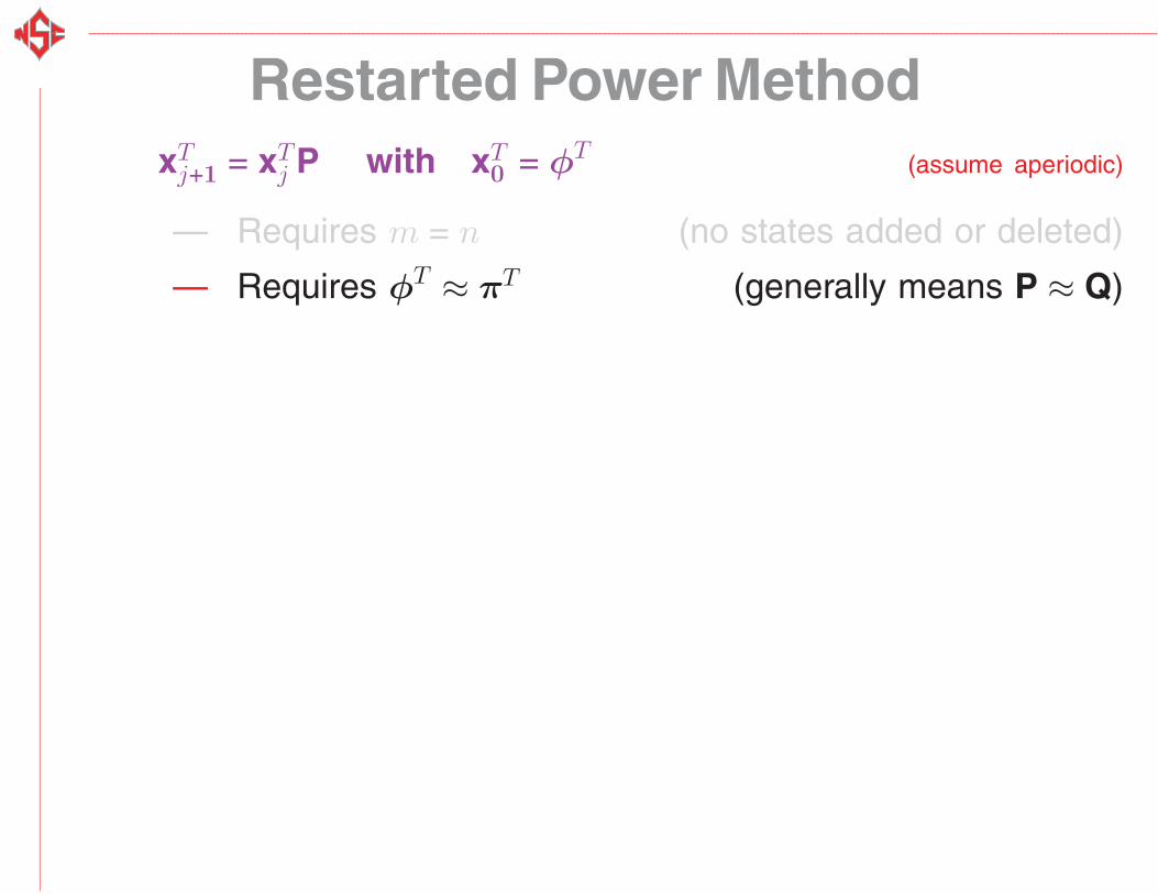
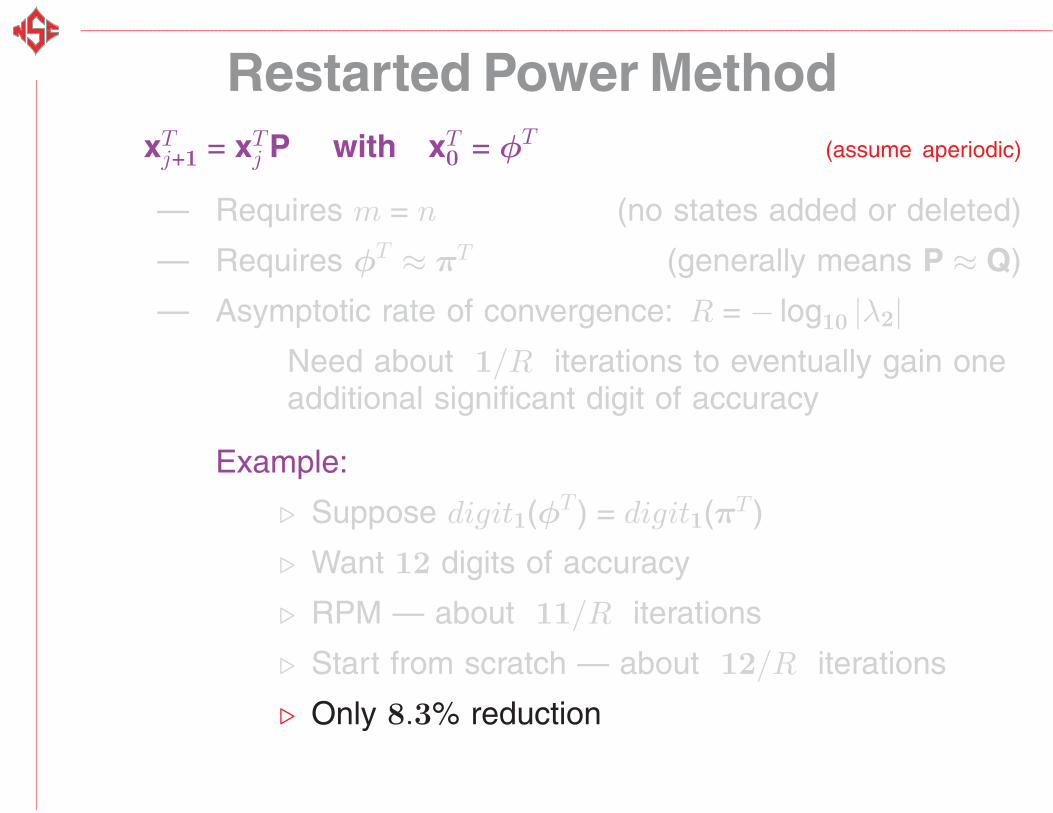
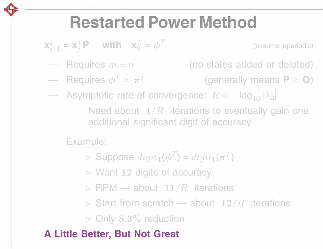
Restarted Power MethodxT
j+1 = xTj P with xT
0 = φT(assume aperiodic)
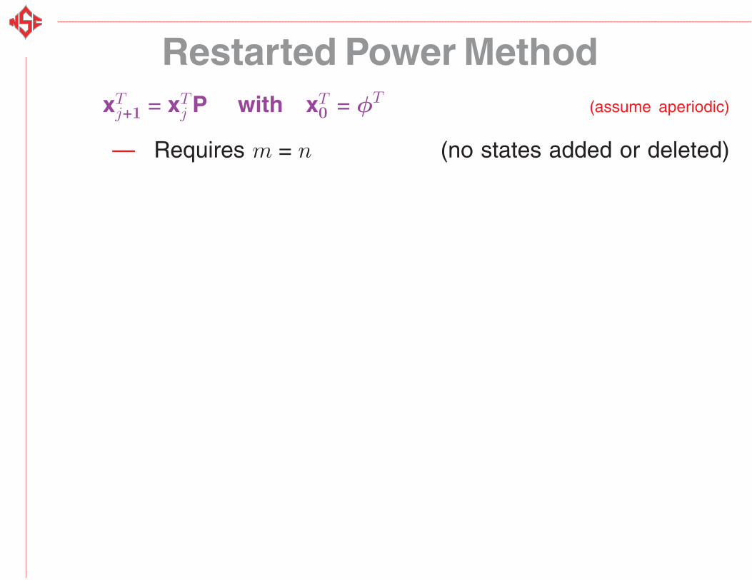
Restarted Power MethodxT
j+1 = xTj P with xT
0 = φT(assume aperiodic)
— Requires m = n (no states added or deleted)
Restarted Power MethodxT
j+1 = xTj P with xT
0 = φT(assume aperiodic)
— Requires m = n (no states added or deleted)
— Requires φT ≈ πT (generally means P ≈ Q)
Restarted Power MethodxT
j+1 = xTj P with xT
0 = φT(assume aperiodic)
— Requires m = n (no states added or deleted)
— Requires φT ≈ πT (generally means P ≈ Q)
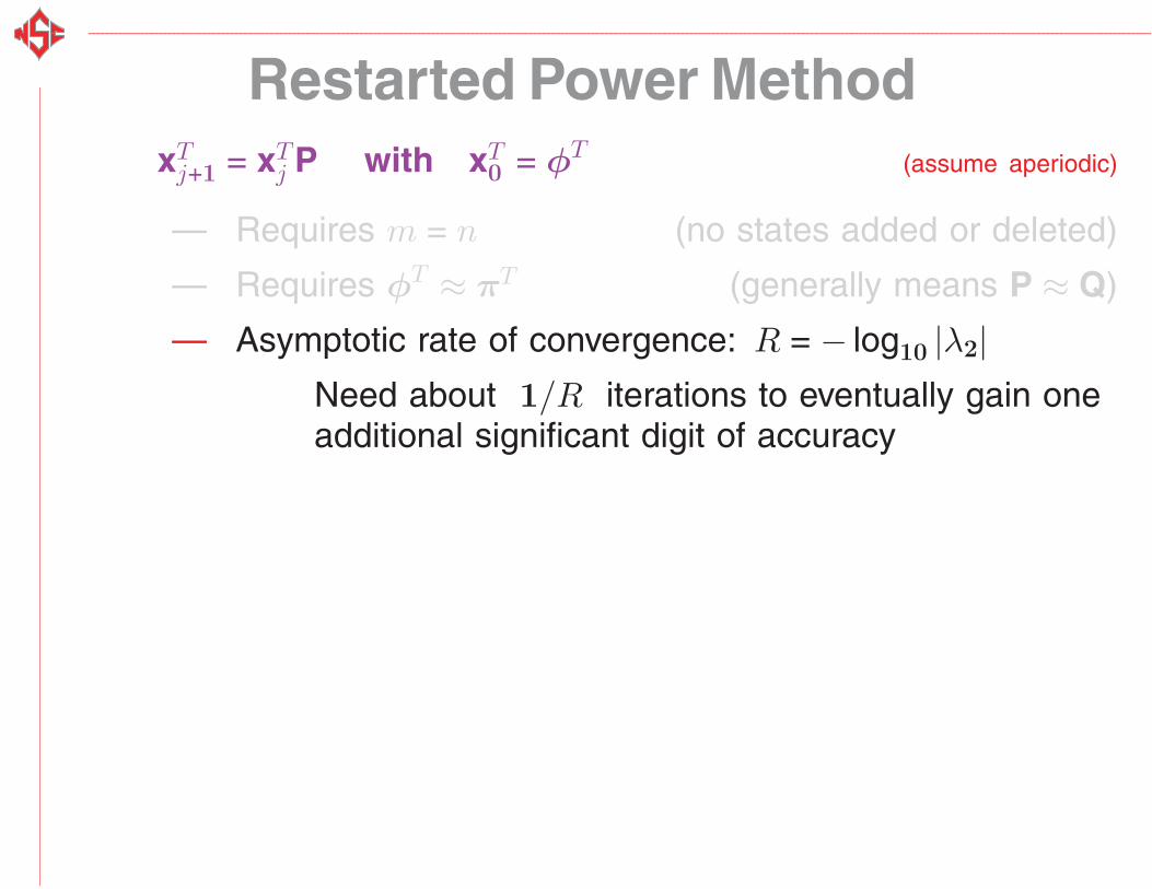
— Asymptotic rate of convergence: R = − log10 |λ2|Need about 1/R iterations to eventually gain oneadditional significant digit of accuracy
Restarted Power MethodxT
j+1 = xTj P with xT
0 = φT(assume aperiodic)
— Requires m = n (no states added or deleted)
— Requires φT ≈ πT (generally means P ≈ Q)
— Asymptotic rate of convergence: R = − log10 |λ2|Need about 1/R iterations to eventually gain oneadditional significant digit of accuracy
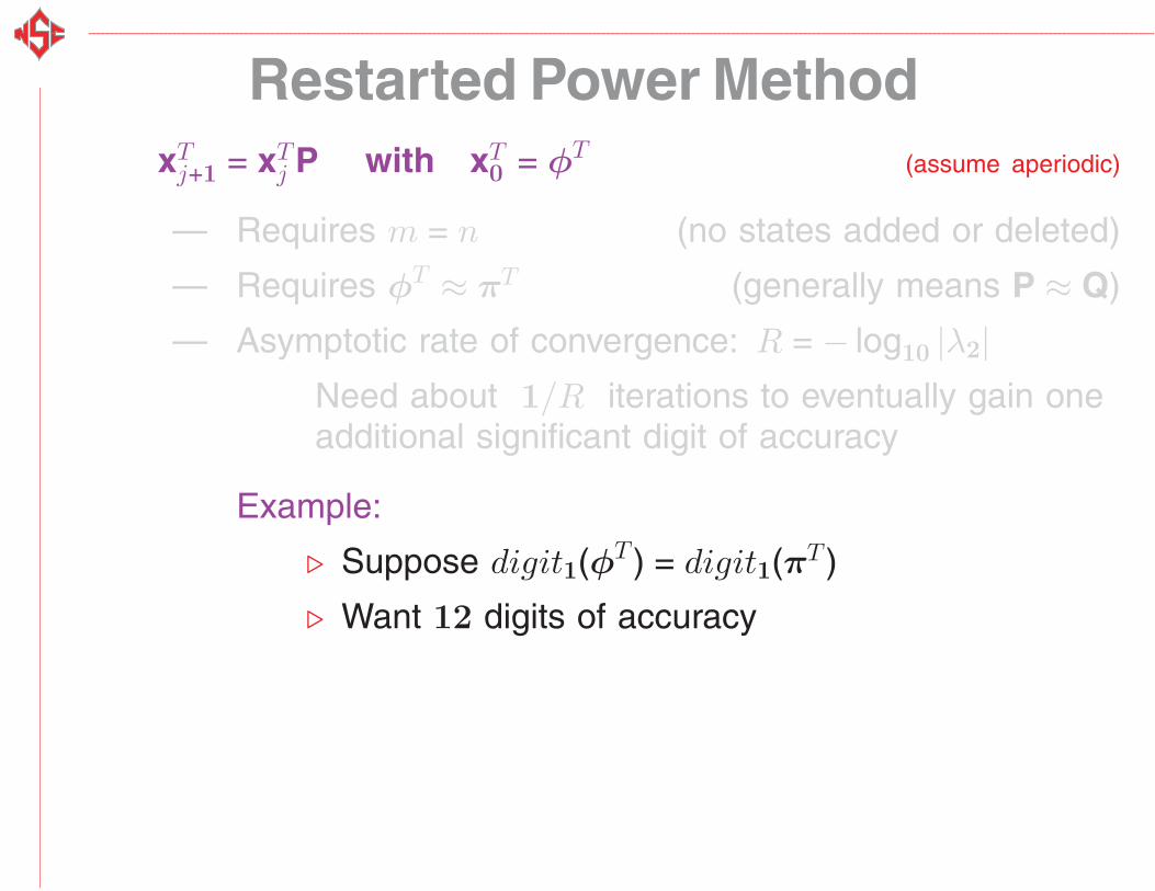
Example:
� Suppose digit1(φT ) = digit1(πT )
� Want 12 digits of accuracy
Restarted Power MethodxT
j+1 = xTj P with xT
0 = φT(assume aperiodic)
— Requires m = n (no states added or deleted)
— Requires φT ≈ πT (generally means P ≈ Q)
— Asymptotic rate of convergence: R = − log10 |λ2|Need about 1/R iterations to eventually gain oneadditional significant digit of accuracy
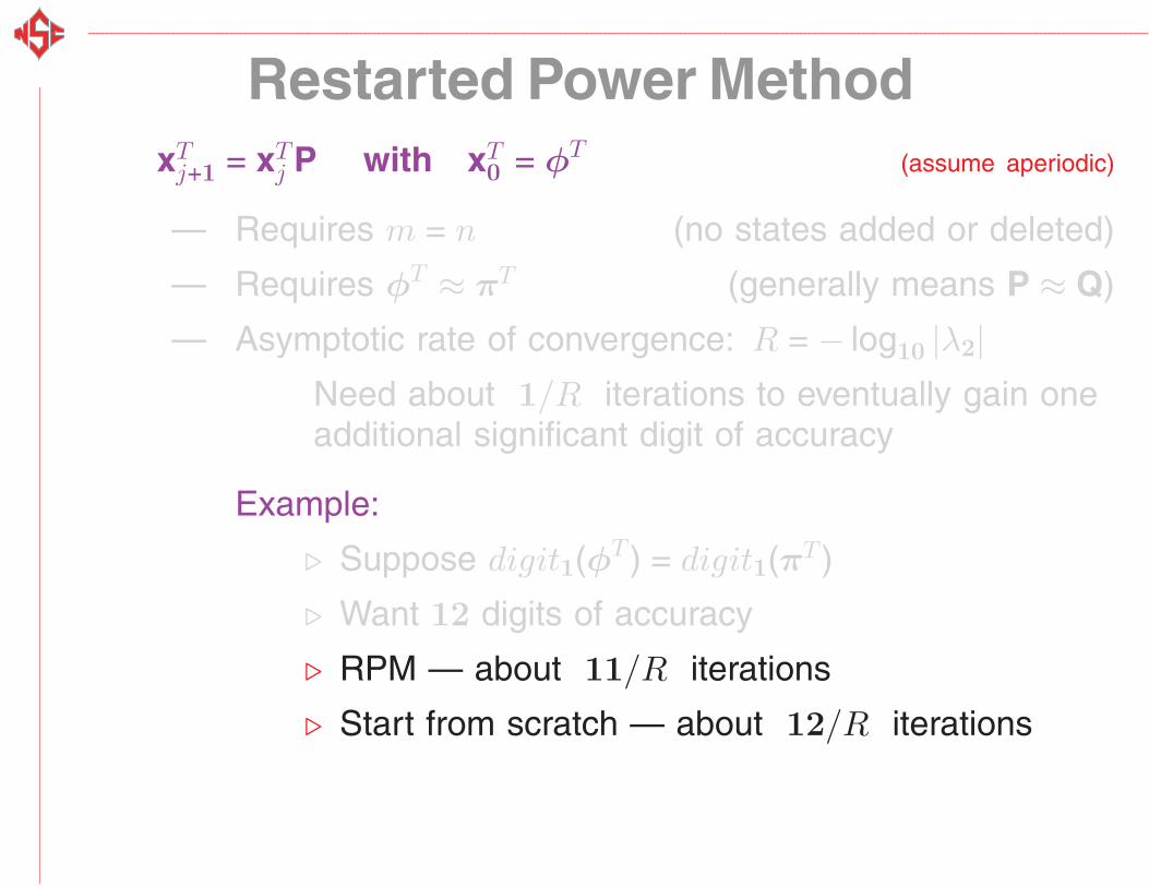
Example:
� Suppose digit1(φT ) = digit1(πT )
� Want 12 digits of accuracy
� RPM — about 11/R iterations
� Start from scratch — about 12/R iterations
Restarted Power MethodxT
j+1 = xTj P with xT
0 = φT(assume aperiodic)
— Requires m = n (no states added or deleted)
— Requires φT ≈ πT (generally means P ≈ Q)
— Asymptotic rate of convergence: R = − log10 |λ2|Need about 1/R iterations to eventually gain oneadditional significant digit of accuracy
Example:
� Suppose digit1(φT ) = digit1(πT )
� Want 12 digits of accuracy
� RPM — about 11/R iterations
� Start from scratch — about 12/R iterations
� Only 8.3% reduction
A Little Better, But Not Great
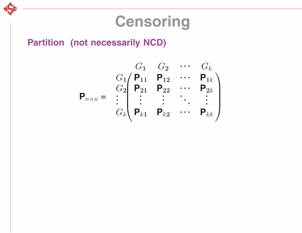
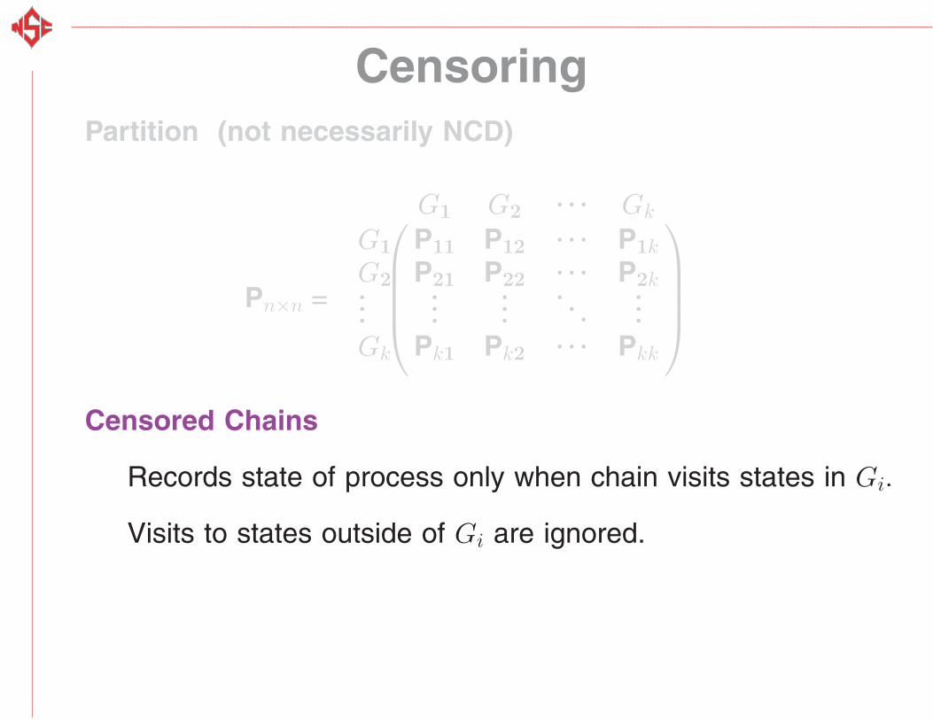
CensoringPartition (not necessarily NCD)
Pn×n =
⎛⎜⎜⎜⎝
G1 G2. . . Gk
G1 P11 P12. . . P1k
G2 P21 P22. . . P2k...
......
. . ....
Gk Pk1 Pk2. . . Pkk
⎞⎟⎟⎟⎠
CensoringPartition (not necessarily NCD)
Pn×n =
⎛⎜⎜⎜⎝
G1 G2. . . Gk
G1 P11 P12. . . P1k
G2 P21 P22. . . P2k...
......
. . ....
Gk Pk1 Pk2. . . Pkk
⎞⎟⎟⎟⎠
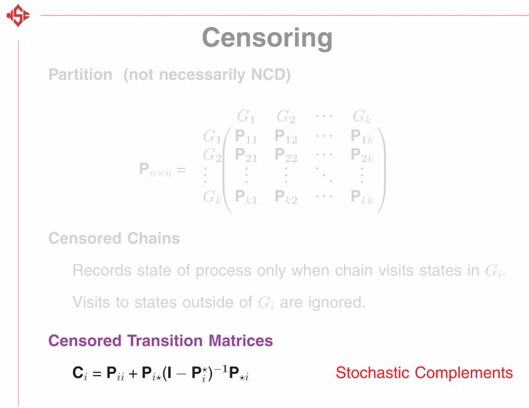
Censored Chains
Records state of process only when chain visits states in Gi.
Visits to states outside of Gi are ignored.
CensoringPartition (not necessarily NCD)
Pn×n =
⎛⎜⎜⎜⎝
G1 G2. . . Gk
G1 P11 P12. . . P1k
G2 P21 P22. . . P2k...
......
. . ....
Gk Pk1 Pk2. . . Pkk
⎞⎟⎟⎟⎠
Censored Chains
Records state of process only when chain visits states in Gi.
Visits to states outside of Gi are ignored.
Censored Transition Matrices
Ci = Pii + Pi�(I − P�i )−1P�i Stochastic Complements
Aggregation
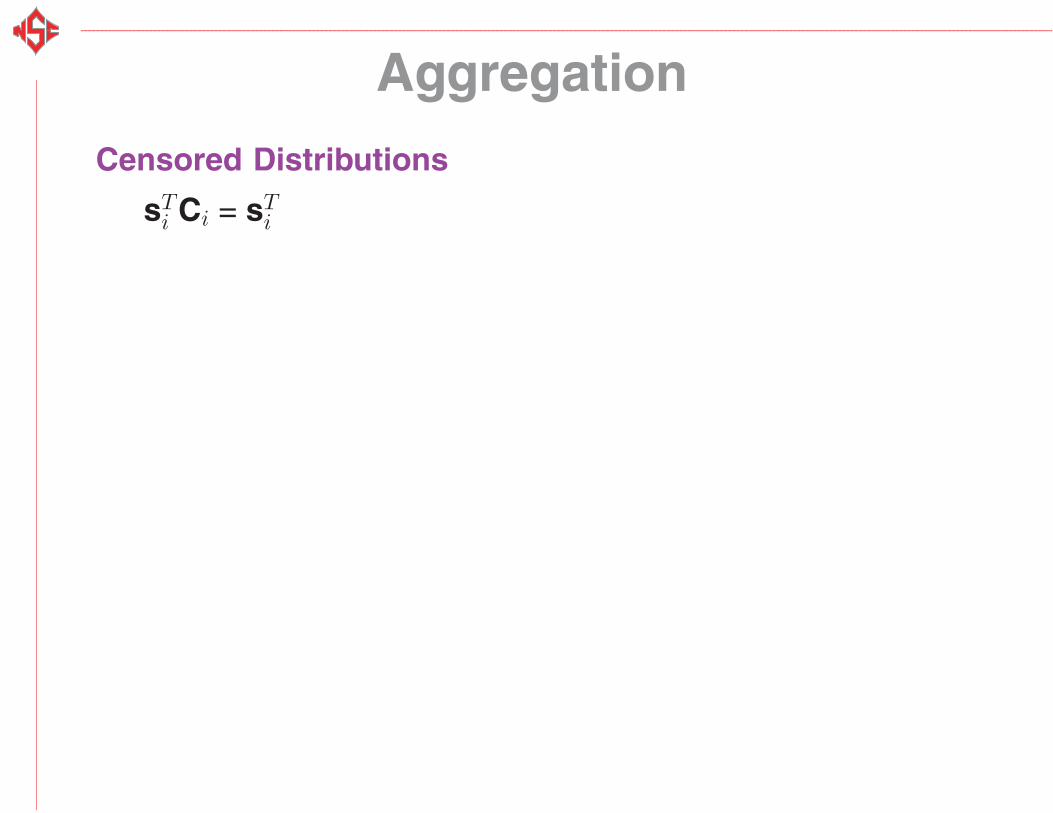
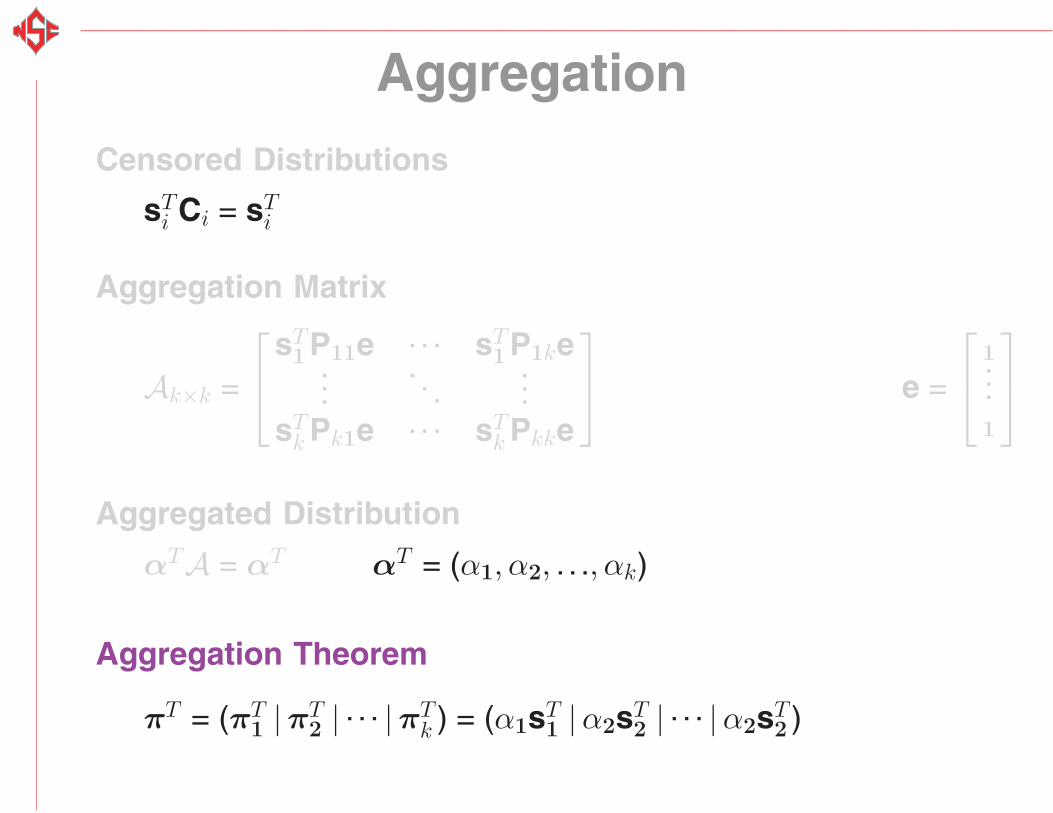
Censored Distributions
sTi Ci = sT
i
Aggregation
Censored Distributions
sTi Ci = sT
i
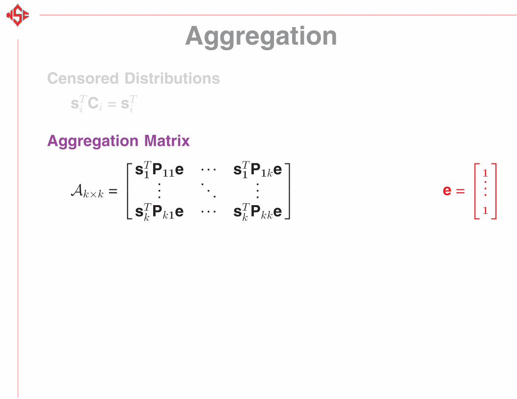
Aggregation Matrix
Ak×k =
⎡⎣ sT
1P11e . . . sT1P1ke
.... . .
...sT
k Pk1e . . . sTk Pkke
⎤⎦ e =
⎡⎣ 1...
1
⎤⎦
Aggregation
Censored Distributions
sTi Ci = sT
i
Aggregation Matrix
Ak×k =
⎡⎣ sT
1P11e . . . sT1P1ke
.... . .
...sT
k Pk1e . . . sTk Pkke
⎤⎦ e =
⎡⎣ 1...
1
⎤⎦
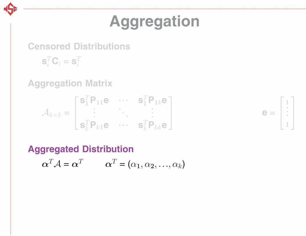
Aggregated Distribution
αTA = αT αT = (α1, α2, . . ., αk)
Aggregation
Censored Distributions
sTi Ci = sT
i
Aggregation Matrix
Ak×k =
⎡⎣ sT
1P11e . . . sT1P1ke
.... . .
...sT
k Pk1e . . . sTk Pkke
⎤⎦ e =
⎡⎣ 1...
1
⎤⎦
Aggregated Distribution
αTA = αT αT = (α1, α2, . . ., αk)
Aggregation Theorem
πT = (πT1 |πT
2 | . . . |πTk ) = (α1sT
1 |α2sT2 | . . . |α2sT
2 )
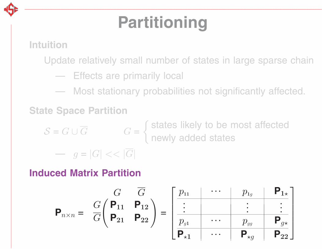
PartitioningIntuition
Update relatively small number of states in large sparse chain
— Effects are primarily local
— Most stationary probabilities not significantly affected.
PartitioningIntuition
Update relatively small number of states in large sparse chain
— Effects are primarily local
— Most stationary probabilities not significantly affected.
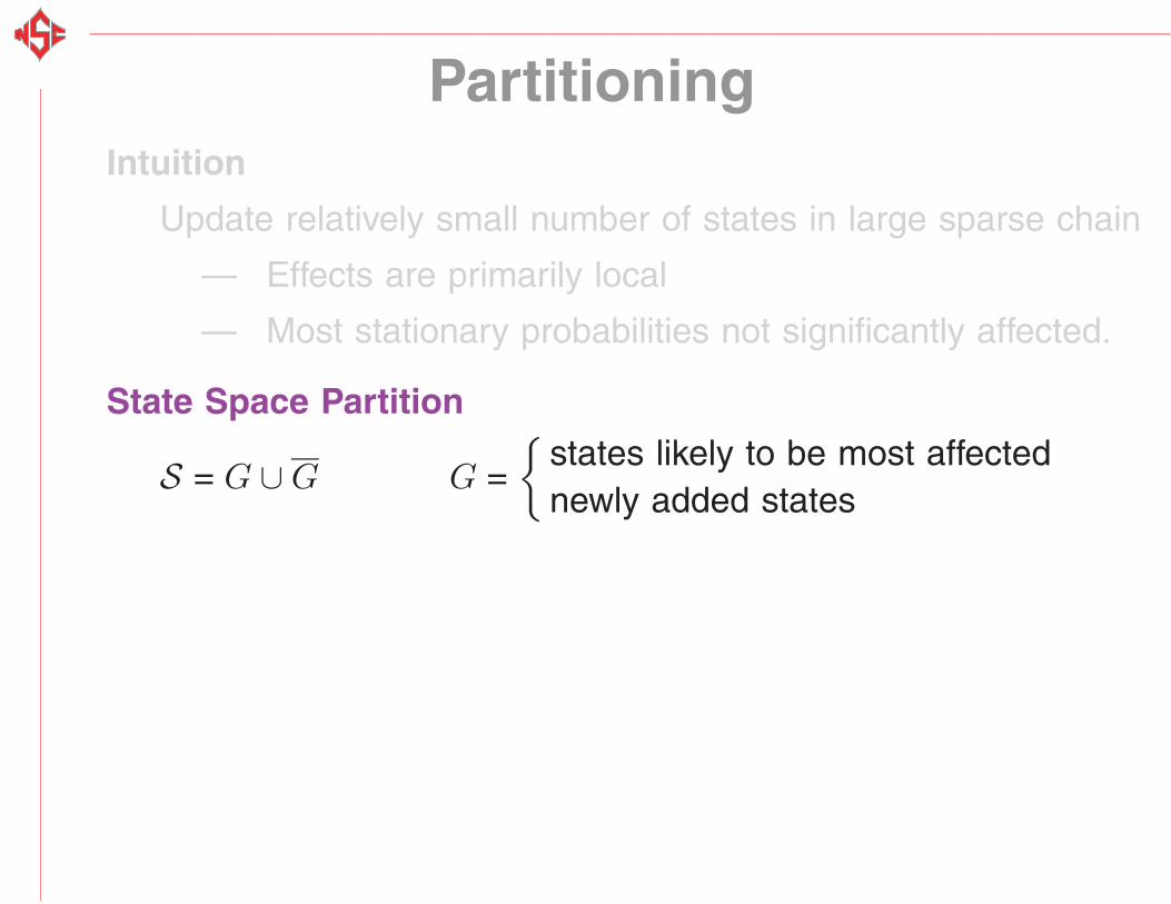
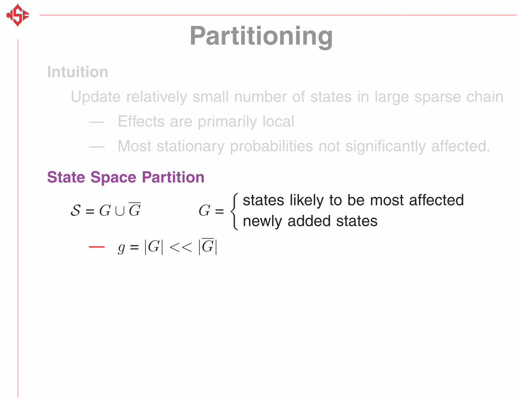
State Space Partition
S = G ∪ G G ={
states likely to be most affectednewly added states
PartitioningIntuition
Update relatively small number of states in large sparse chain
— Effects are primarily local
— Most stationary probabilities not significantly affected.
State Space Partition
S = G ∪ G G ={
states likely to be most affectednewly added states
— g = |G| << |G|
PartitioningIntuition
Update relatively small number of states in large sparse chain
— Effects are primarily local
— Most stationary probabilities not significantly affected.
State Space Partition
S = G ∪ G G ={
states likely to be most affectednewly added states
— g = |G| << |G|
Induced Matrix Partition
Pn×n =
( G GG P11 P12
G P21 P22
)=
⎡⎢⎢⎢⎣
p11. . . p1g P1�
......
...pg1
. . . pgg Pg�
P�1. . . P�g P22
⎤⎥⎥⎥⎦
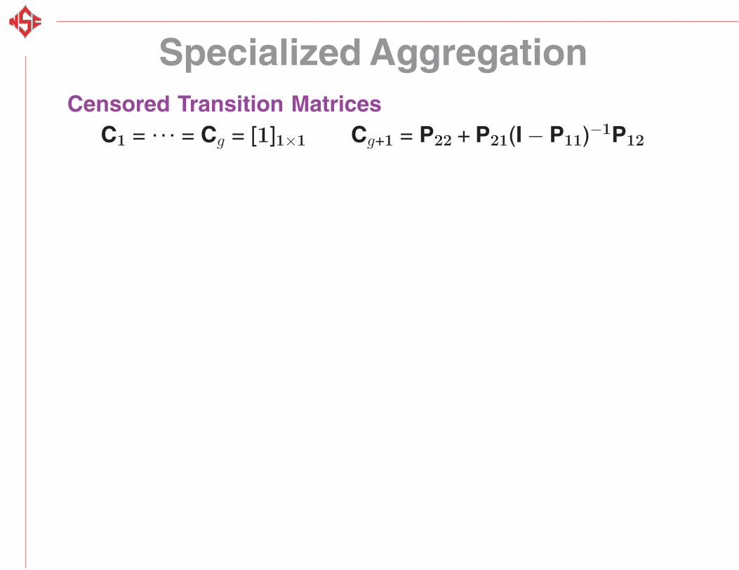
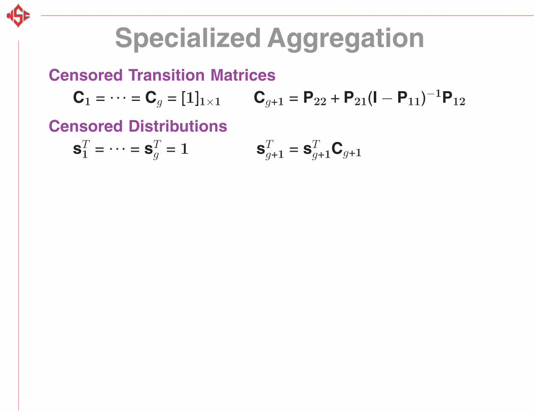
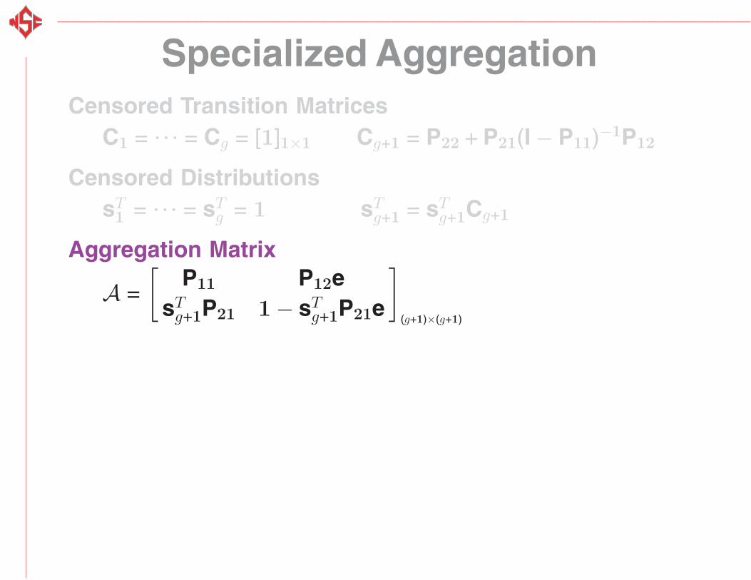
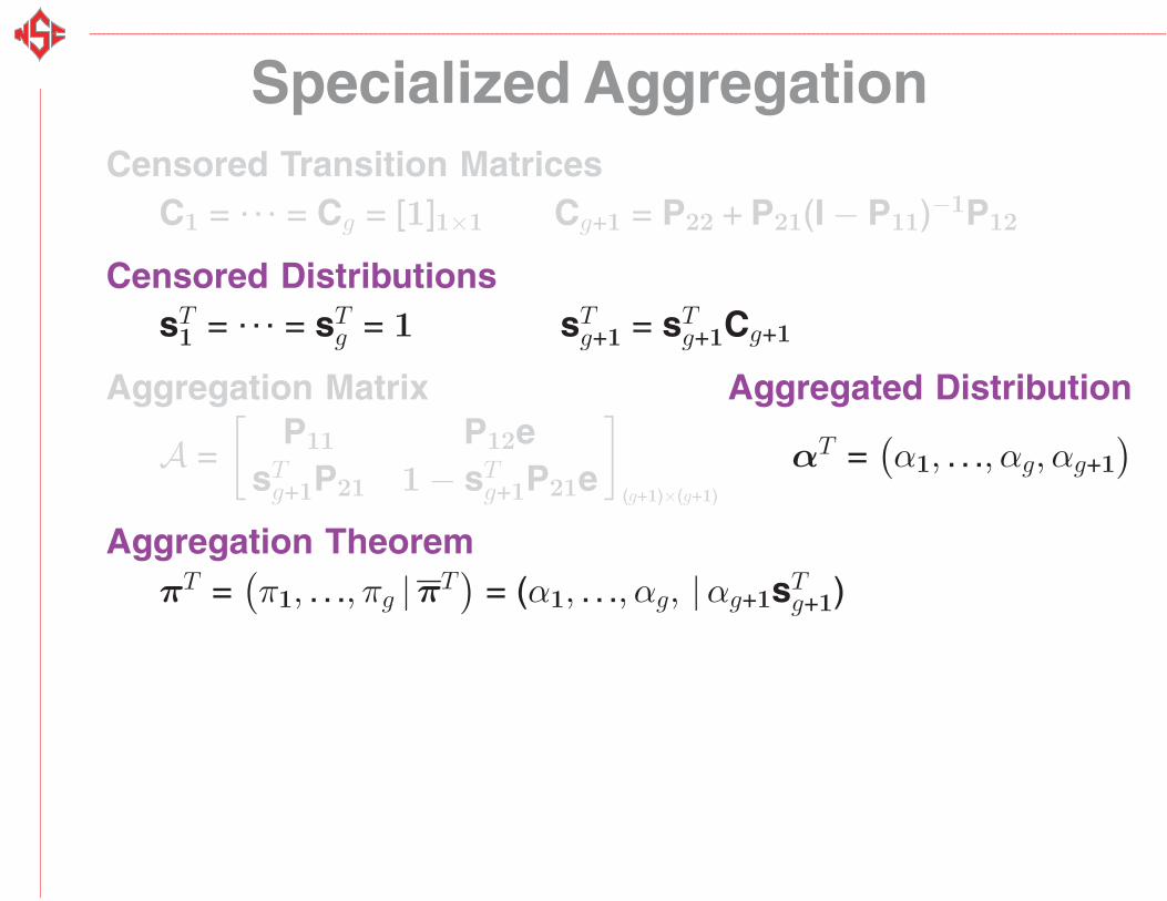
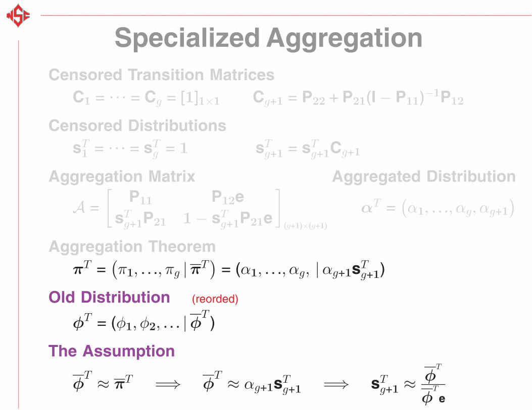
Specialized AggregationCensored Transition Matrices
C1 = . . . = Cg = [1]1×1 Cg+1 = P22 + P21(I − P11)−1P12
Specialized AggregationCensored Transition Matrices
C1 = . . . = Cg = [1]1×1 Cg+1 = P22 + P21(I − P11)−1P12
Censored DistributionssT
1 = . . . = sTg = 1 sT
g+1 = sTg+1Cg+1
Specialized AggregationCensored Transition Matrices
C1 = . . . = Cg = [1]1×1 Cg+1 = P22 + P21(I − P11)−1P12
Censored DistributionssT
1 = . . . = sTg = 1 sT
g+1 = sTg+1Cg+1
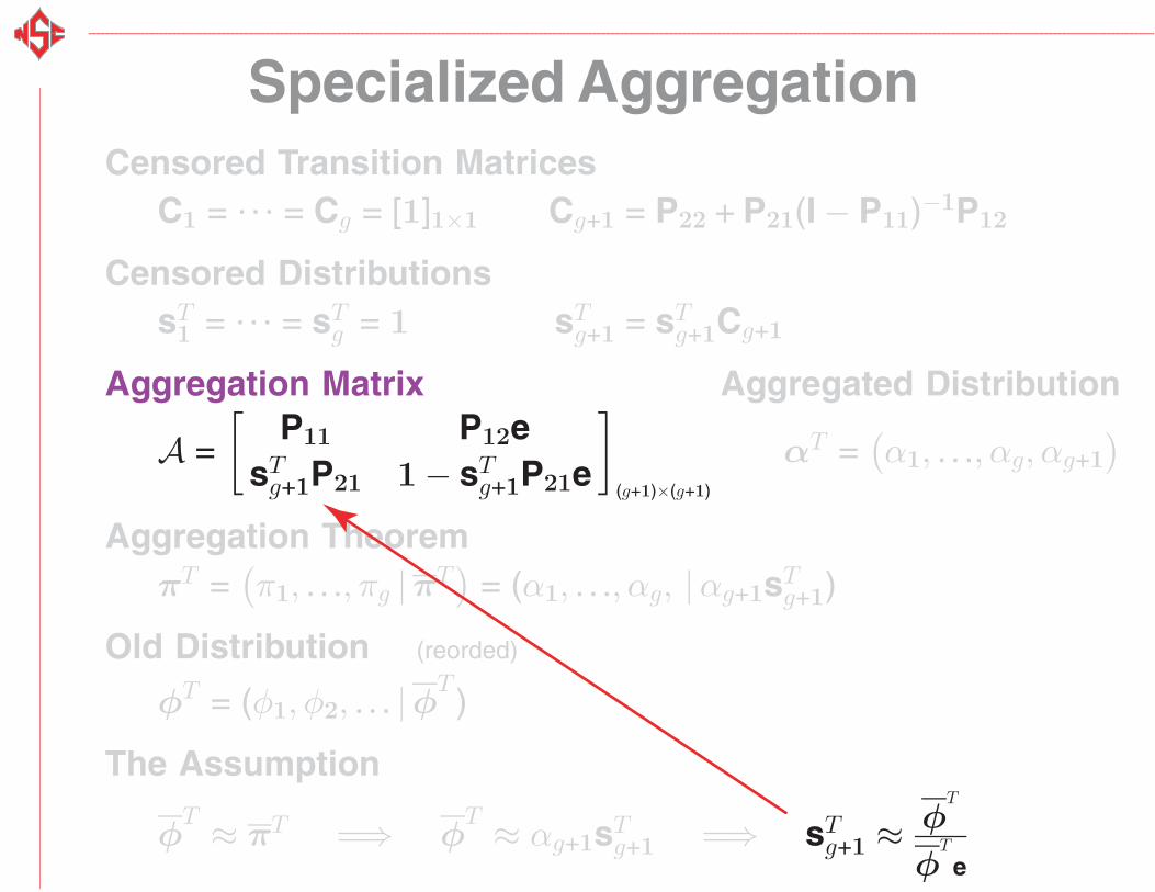
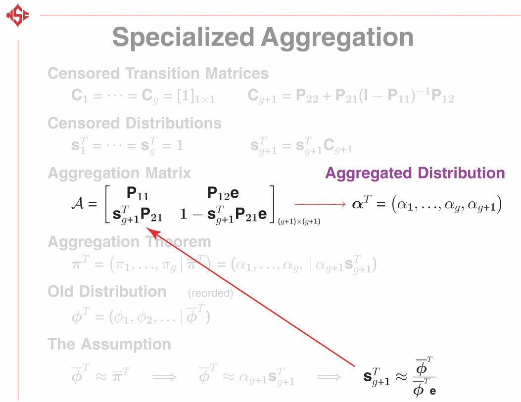
Aggregation Matrix
A =[
P11 P12esT
g+1P21 1 − sTg+1P21e
](g+1)×(g+1)
Specialized AggregationCensored Transition Matrices
C1 = . . . = Cg = [1]1×1 Cg+1 = P22 + P21(I − P11)−1P12
Censored DistributionssT
1 = . . . = sTg = 1 sT
g+1 = sTg+1Cg+1
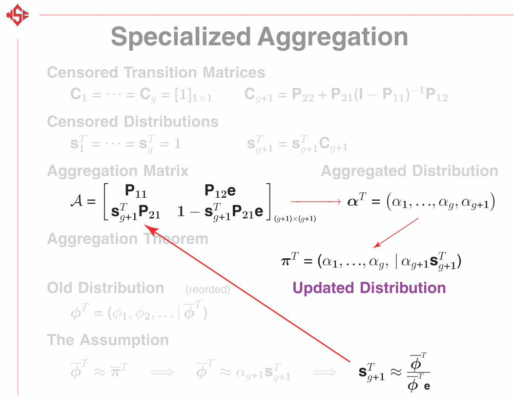
Aggregation Matrix Aggregated Distribution
A =[
P11 P12esT
g+1P21 1 − sTg+1P21e
](g+1)×(g+1)
αT =(α1, . . ., αg, αg+1
)Aggregation Theorem
πT =(π1, . . ., πg |πT
)= (α1, . . ., αg, |αg+1sT
g+1)
Specialized AggregationCensored Transition Matrices
C1 = . . . = Cg = [1]1×1 Cg+1 = P22 + P21(I − P11)−1P12
Censored DistributionssT
1 = . . . = sTg = 1 sT
g+1 = sTg+1Cg+1
Aggregation Matrix Aggregated Distribution
A =[
P11 P12esT
g+1P21 1 − sTg+1P21e
](g+1)×(g+1)
αT =(α1, . . ., αg, αg+1
)Aggregation Theorem
πT =(π1, . . ., πg |πT
)= (α1, . . ., αg, |αg+1sT
g+1)
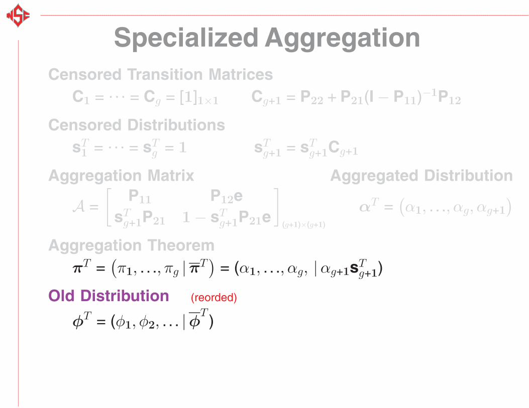
Old Distribution (reorded)
φT = (φ1, φ2, . . . |φT)
Specialized AggregationCensored Transition Matrices
C1 = . . . = Cg = [1]1×1 Cg+1 = P22 + P21(I − P11)−1P12
Censored DistributionssT
1 = . . . = sTg = 1 sT
g+1 = sTg+1Cg+1
Aggregation Matrix Aggregated Distribution
A =[
P11 P12esT
g+1P21 1 − sTg+1P21e
](g+1)×(g+1)
αT =(α1, . . ., αg, αg+1
)Aggregation Theorem
πT =(π1, . . ., πg |πT
)= (α1, . . ., αg, |αg+1sT
g+1)
Old Distribution (reorded)
φT = (φ1, φ2, . . . |φT)
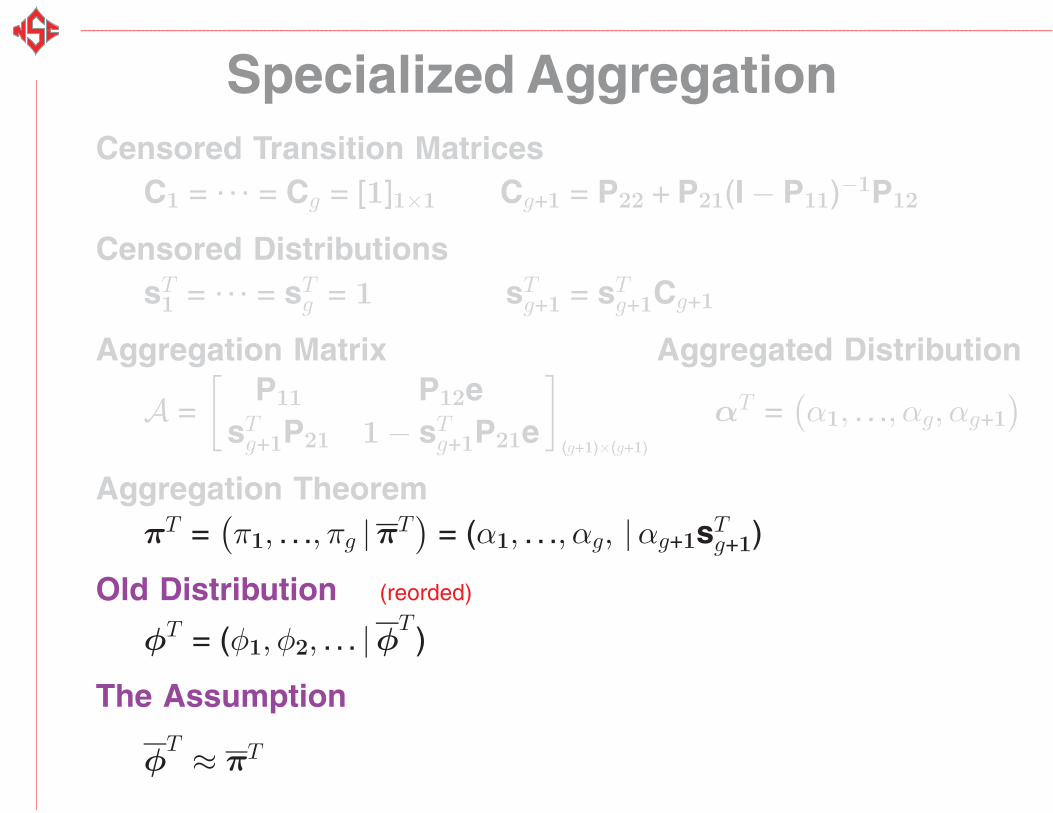
The Assumption
φT ≈ πT
Specialized AggregationCensored Transition Matrices
C1 = . . . = Cg = [1]1×1 Cg+1 = P22 + P21(I − P11)−1P12
Censored DistributionssT
1 = . . . = sTg = 1 sT
g+1 = sTg+1Cg+1
Aggregation Matrix Aggregated Distribution
A =[
P11 P12esT
g+1P21 1 − sTg+1P21e
](g+1)×(g+1)
αT =(α1, . . ., αg, αg+1
)Aggregation Theorem
πT =(π1, . . ., πg |πT
)= (α1, . . ., αg, |αg+1sT
g+1)
Old Distribution (reorded)
φT = (φ1, φ2, . . . |φT)
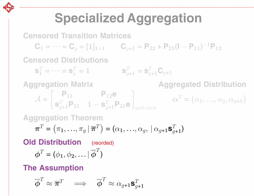
The Assumption
φT ≈ πT =⇒ φ
T ≈ αg+1sTg+1
Specialized AggregationCensored Transition Matrices
C1 = . . . = Cg = [1]1×1 Cg+1 = P22 + P21(I − P11)−1P12
Censored DistributionssT
1 = . . . = sTg = 1 sT
g+1 = sTg+1Cg+1
Aggregation Matrix Aggregated Distribution
A =[
P11 P12esT
g+1P21 1 − sTg+1P21e
](g+1)×(g+1)
αT =(α1, . . ., αg, αg+1
)Aggregation Theorem
πT =(π1, . . ., πg |πT
)= (α1, . . ., αg, |αg+1sT
g+1)
Old Distribution (reorded)
φT = (φ1, φ2, . . . |φT)
The Assumption
φT ≈ πT =⇒ φ
T ≈ αg+1sTg+1 =⇒ sT
g+1 ≈ φT
φT
e
Specialized AggregationCensored Transition Matrices
C1 = . . . = Cg = [1]1×1 Cg+1 = P22 + P21(I − P11)−1P12
Censored DistributionssT
1 = . . . = sTg = 1 sT
g+1 = sTg+1Cg+1
Aggregation Matrix Aggregated Distribution
A =[
P11 P12esT
g+1P21 1 − sTg+1P21e
](g+1)×(g+1)
−−−−−→ αT =(α1, . . ., αg, αg+1
)Aggregation Theorem
πT = (α1, . . ., αg, |αg+1sTg+1)
Old Distribution (reorded) Updated Distribution
φT = (φ1, φ2, . . . |φT)
The Assumption
φT ≈ πT =⇒ φ
T ≈ αg+1sTg+1 =⇒ sT
g+1 ≈ φT
φT
e
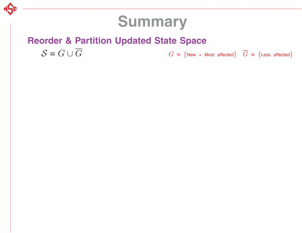
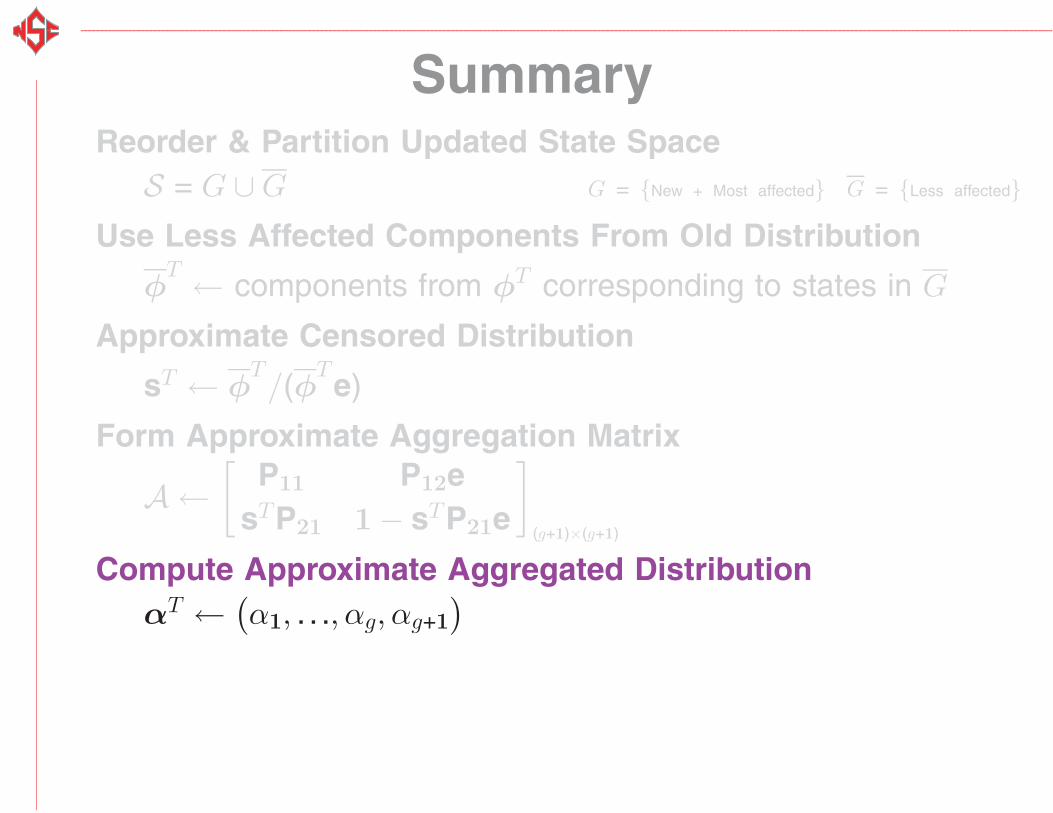
SummaryReorder & Partition Updated State Space
S = G ∪ G G = {New + Most affected} G = {Less affected}
SummaryReorder & Partition Updated State Space
S = G ∪ G G = {New + Most affected} G = {Less affected}
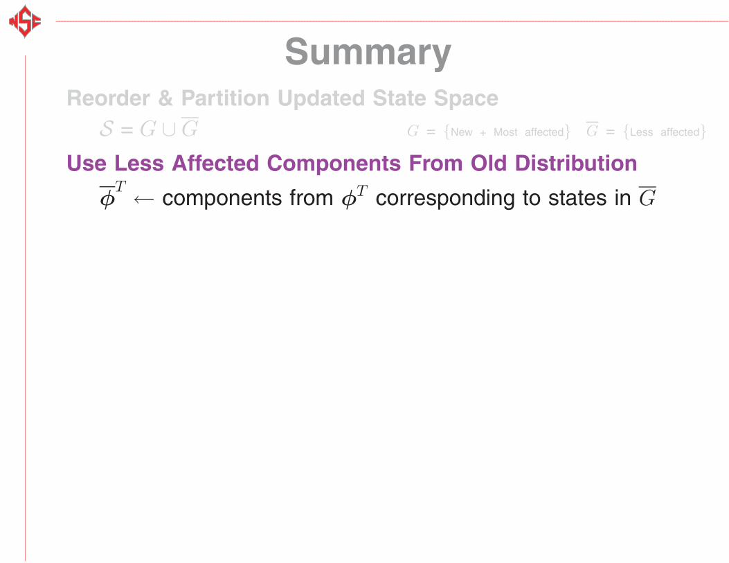
Use Less Affected Components From Old Distribution
φT ← components from φT corresponding to states in G
SummaryReorder & Partition Updated State Space
S = G ∪ G G = {New + Most affected} G = {Less affected}
Use Less Affected Components From Old Distribution
φT ← components from φT corresponding to states in G
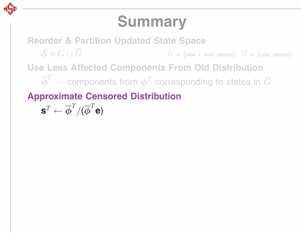
Approximate Censored Distribution
sT ← φT/(φ
Te)
SummaryReorder & Partition Updated State Space
S = G ∪ G G = {New + Most affected} G = {Less affected}
Use Less Affected Components From Old Distribution
φT ← components from φT corresponding to states in G
Approximate Censored Distribution
sT ← φT/(φ
Te)
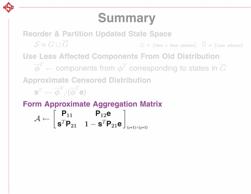
Form Approximate Aggregation Matrix
A ←[
P11 P12esTP21 1 − sTP21e
](g+1)×(g+1)
SummaryReorder & Partition Updated State Space
S = G ∪ G G = {New + Most affected} G = {Less affected}
Use Less Affected Components From Old Distribution
φT ← components from φT corresponding to states in G
Approximate Censored Distribution
sT ← φT/(φ
Te)
Form Approximate Aggregation Matrix
A ←[
P11 P12esTP21 1 − sTP21e
](g+1)×(g+1)
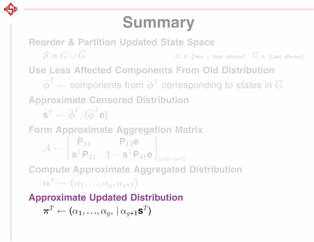
Compute Approximate Aggregated DistributionαT ←
(α1, . . ., αg, αg+1
)
SummaryReorder & Partition Updated State Space
S = G ∪ G G = {New + Most affected} G = {Less affected}
Use Less Affected Components From Old Distribution
φT ← components from φT corresponding to states in G
Approximate Censored Distribution
sT ← φT/(φ
Te)
Form Approximate Aggregation Matrix
A ←[
P11 P12esTP21 1 − sTP21e
](g+1)×(g+1)
Compute Approximate Aggregated DistributionαT ←
(α1, . . ., αg, αg+1
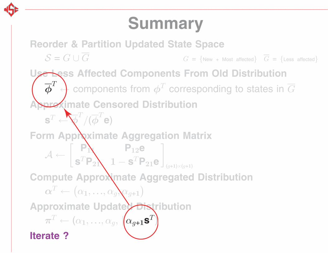
)Approximate Updated Distribution
πT ← (α1, . . ., αg, |αg+1sT )
SummaryReorder & Partition Updated State Space
S = G ∪ G G = {New + Most affected} G = {Less affected}
Use Less Affected Components From Old Distribution
φT ← components from φT corresponding to states in G
Approximate Censored Distribution
sT ← φT/(φ
Te)
Form Approximate Aggregation Matrix
A ←[
P11 P12esTP21 1 − sTP21e
](g+1)×(g+1)
Compute Approximate Aggregated DistributionαT ←
(α1, . . ., αg, αg+1
)Approximate Updated Distribution
πT ← (α1, . . ., αg, |αg+1sT )
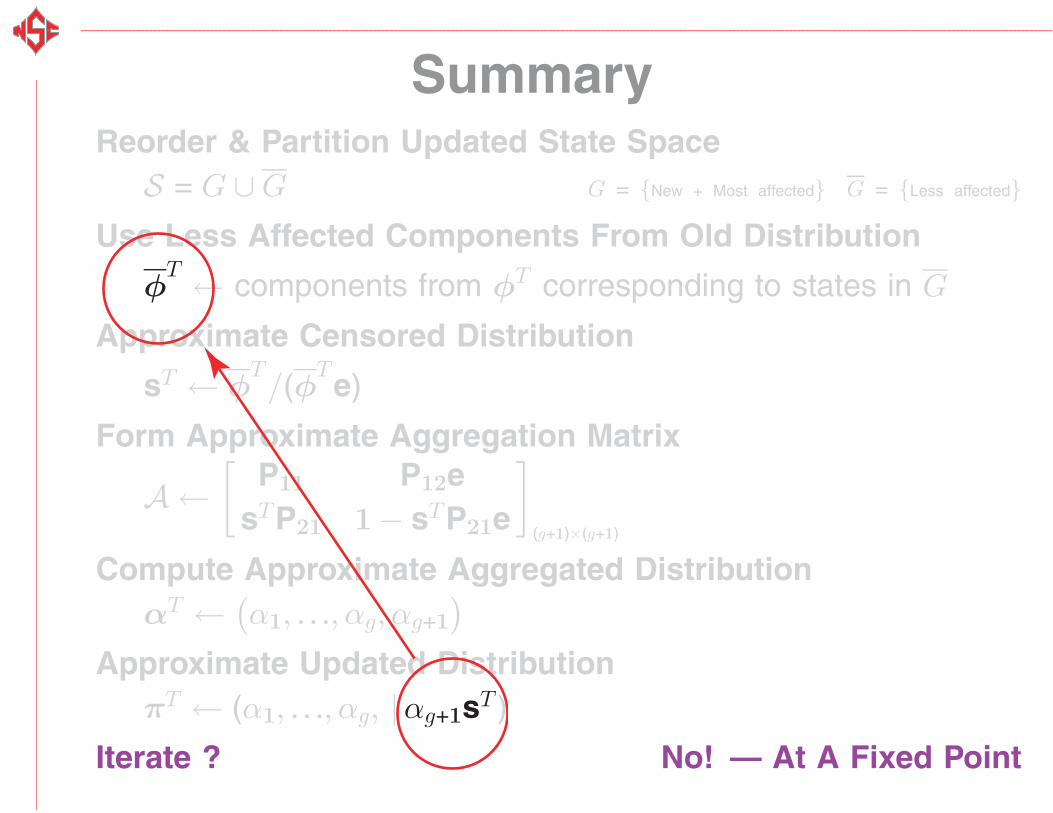
Iterate ?
SummaryReorder & Partition Updated State Space
S = G ∪ G G = {New + Most affected} G = {Less affected}
Use Less Affected Components From Old Distribution
φT ← components from φT corresponding to states in G
Approximate Censored Distribution
sT ← φT/(φ
Te)
Form Approximate Aggregation Matrix
A ←[
P11 P12esTP21 1 − sTP21e
](g+1)×(g+1)
Compute Approximate Aggregated DistributionαT ←
(α1, . . ., αg, αg+1
)Approximate Updated Distribution
πT ← (α1, . . ., αg, |αg+1sT )
Iterate ? No! — At A Fixed Point
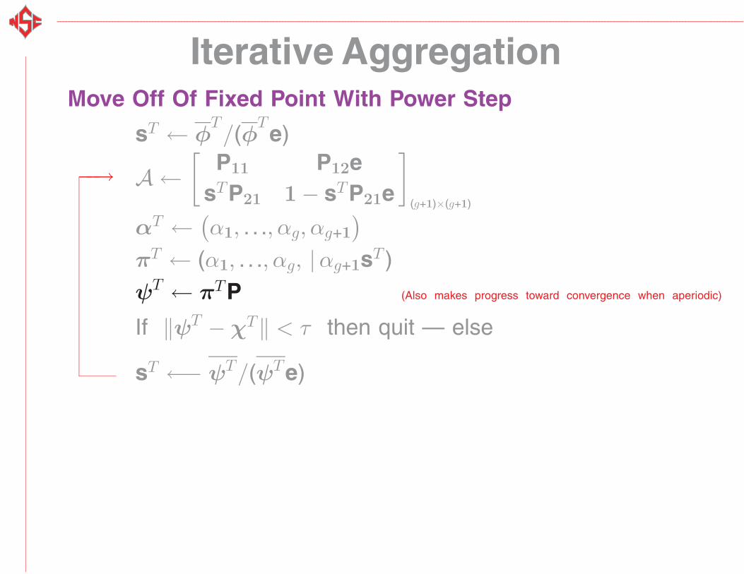
Iterative AggregationMove Off Of Fixed Point With Power Step
sT ← φT/(φ
Te)
A ←[
P11 P12esTP21 1 − sTP21e
](g+1)×(g+1)
αT ←(α1, . . ., αg, αg+1
)πT ← (α1, . . ., αg, |αg+1sT )ψT ← πTP (Also makes progress toward convergence when aperiodic)
If ‖ψT − χT‖ < τ then quit — else
sT ←− ψT/(ψTe)
−−→
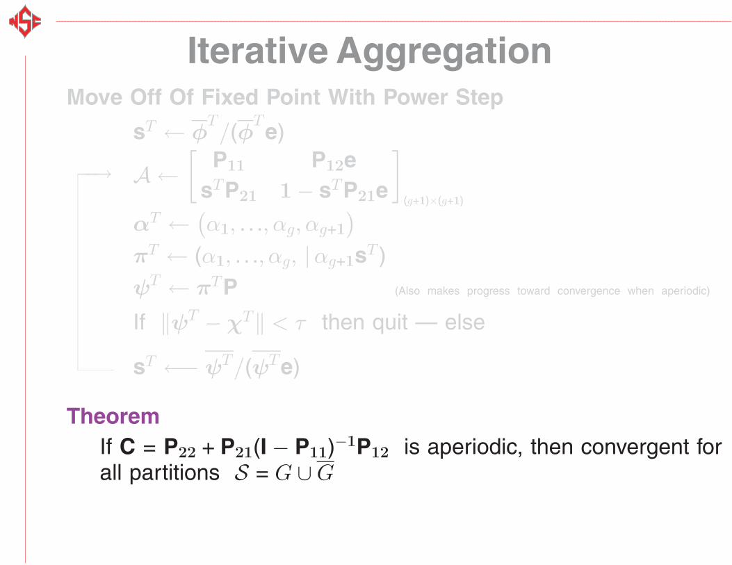
Iterative AggregationMove Off Of Fixed Point With Power Step
sT ← φT/(φ
Te)
A ←[
P11 P12esTP21 1 − sTP21e
](g+1)×(g+1)
αT ←(α1, . . ., αg, αg+1
)πT ← (α1, . . ., αg, |αg+1sT )ψT ← πTP (Also makes progress toward convergence when aperiodic)
If ‖ψT − χT‖ < τ then quit — else
sT ←− ψT/(ψTe)
−−→
TheoremIf C = P22 + P21(I − P11)−1P12 is aperiodic, then convergent forall partitions S = G ∪ G
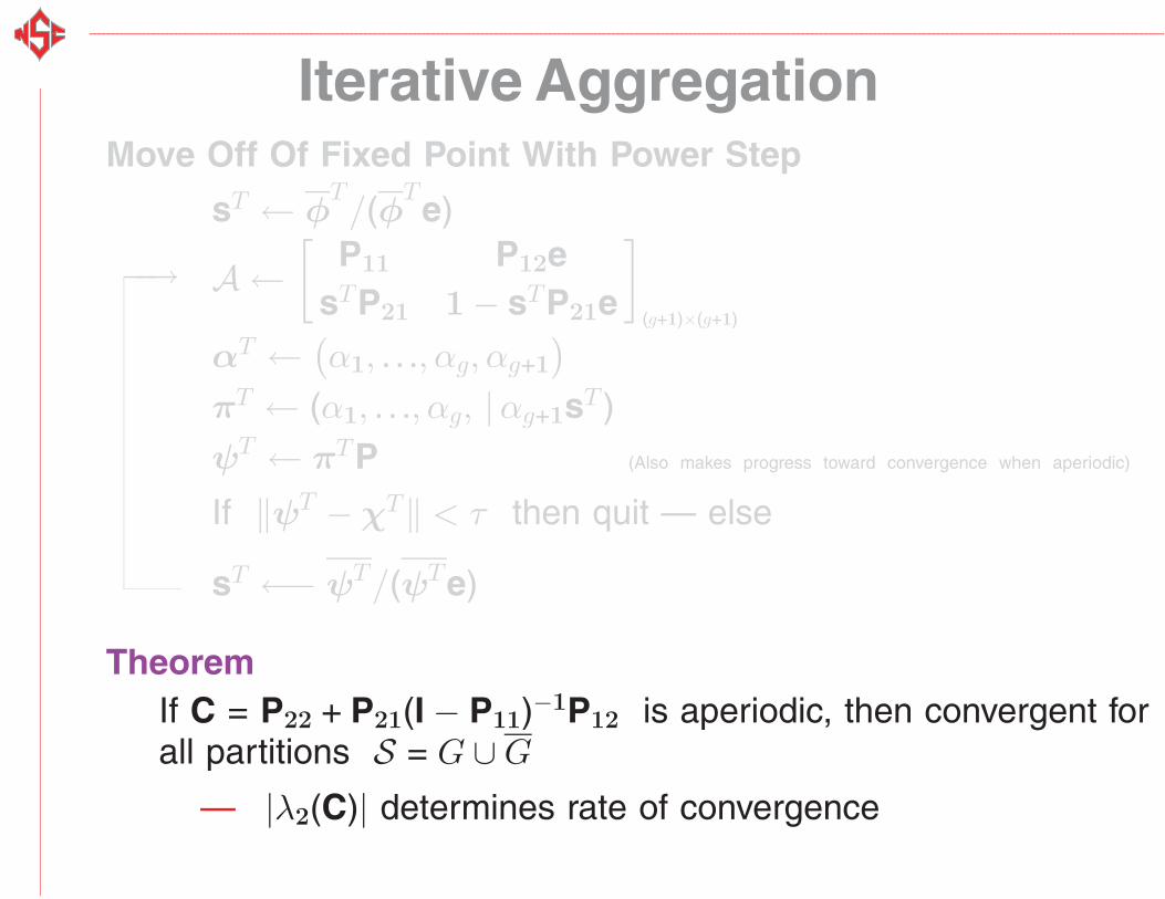
— |λ2(C)| determines rate of convergence
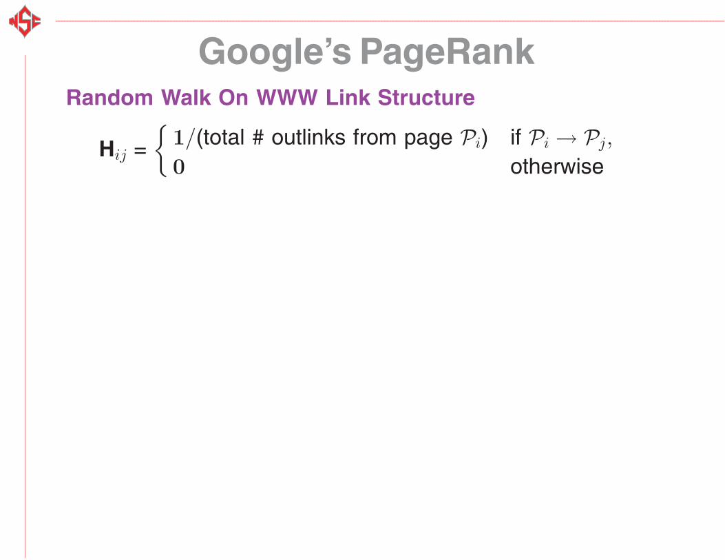
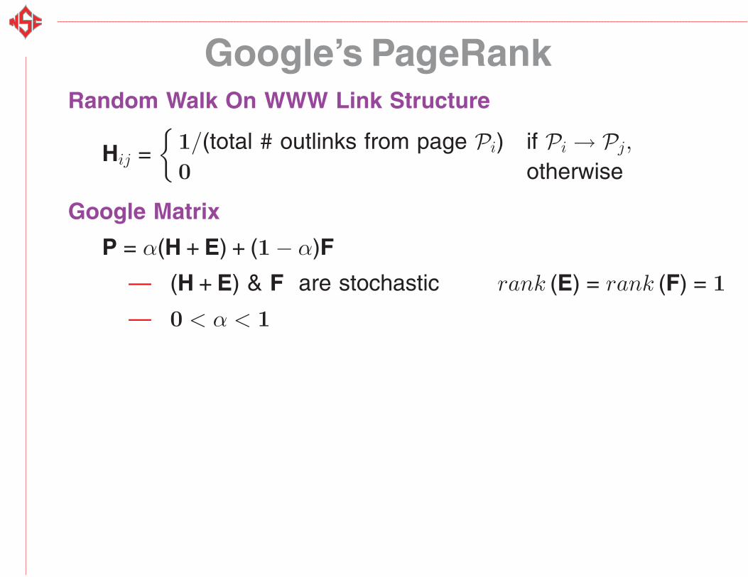
Google’s PageRankRandom Walk On WWW Link Structure
Hij ={
1/(total # outlinks from page Pi) if Pi → Pj,
0 otherwise
Google’s PageRankRandom Walk On WWW Link Structure
Hij ={
1/(total # outlinks from page Pi) if Pi → Pj,
0 otherwise
Google Matrix
P = α(H + E) + (1 − α)F
— (H + E) & F are stochastic rank (E) = rank (F) = 1
— 0 < α < 1

Google’s PageRankRandom Walk On WWW Link Structure
Hij ={
1/(total # outlinks from page Pi) if Pi → Pj,
0 otherwise
Google Matrix
P = α(H + E) + (1 − α)F
— (H + E) & F are stochastic rank (E) = rank (F) = 1
— 0 < α < 1
— PageRank = πT
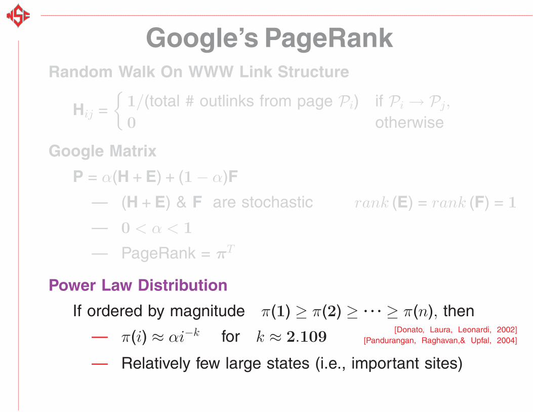
Google’s PageRankRandom Walk On WWW Link Structure
Hij ={
1/(total # outlinks from page Pi) if Pi → Pj,
0 otherwise
Google Matrix
P = α(H + E) + (1 − α)F
— (H + E) & F are stochastic rank (E) = rank (F) = 1
— 0 < α < 1
— PageRank = πT
Power Law Distribution
If ordered by magnitude π(1) ≥ π(2) ≥ . . . ≥ π(n), then
— π(i) ≈ αi−k for k ≈ 2.109[Donato, Laura, Leonardi, 2002]
[Pandurangan, Raghavan,& Upfal, 2004]
— Relatively few large states (i.e., important sites)
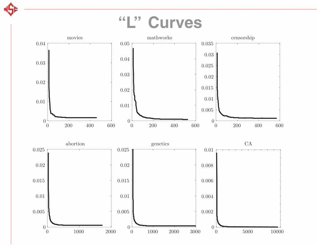
“L” Curves
0 200 400 6000
0.005
0.01
0.015
0.02
0.025
0.03
0.035censorship
0 200 400 6000
0.01
0.02
0.03
0.04movies
0 200 400 6000
0.01
0.02
0.03
0.04
0.05mathworks
0 1000 2000 0 5000 100000
0.005
0.01
0.015
0.02
0.025abortion
0 1000 2000 30000
0.005
0.01
0.015
0.02
0.025
0
0.002
0.004
0.008
0.006
0.01genetics CA
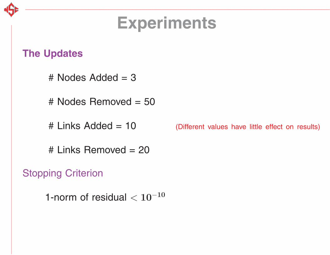
Experiments
The Updates
# Nodes Added = 3
# Nodes Removed = 50
# Links Added = 10 (Different values have little effect on results)
# Links Removed = 20
Stopping Criterion
1-norm of residual < 10−10
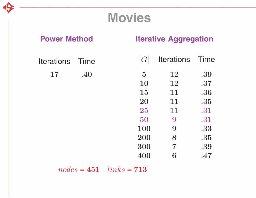
Movies
Power Method Iterative Aggregation
Iterations Time
17 .40
|G| Iterations Time
5 12 .3910 12 .3715 11 .3620 11 .3525 11 .3150 9 .31100 9 .33200 8 .35300 7 .39400 6 .47
nodes = 451 links = 713
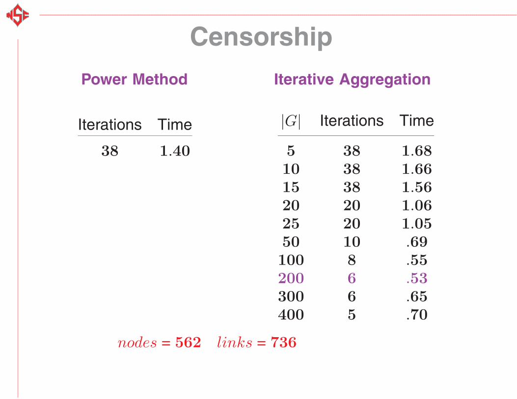
Censorship
Power Method Iterative Aggregation
Iterations Time
38 1.40
|G| Iterations Time
5 38 1.6810 38 1.6615 38 1.5620 20 1.0625 20 1.0550 10 .69100 8 .55200 6 .53300 6 .65400 5 .70
nodes = 562 links = 736
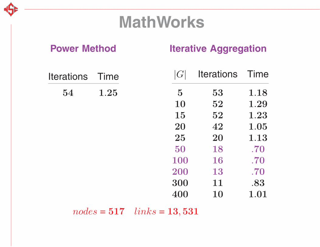
MathWorks
Power Method Iterative Aggregation
Iterations Time
54 1.25
|G| Iterations Time
5 53 1.1810 52 1.2915 52 1.2320 42 1.0525 20 1.1350 18 .70100 16 .70200 13 .70300 11 .83400 10 1.01
nodes = 517 links = 13,531
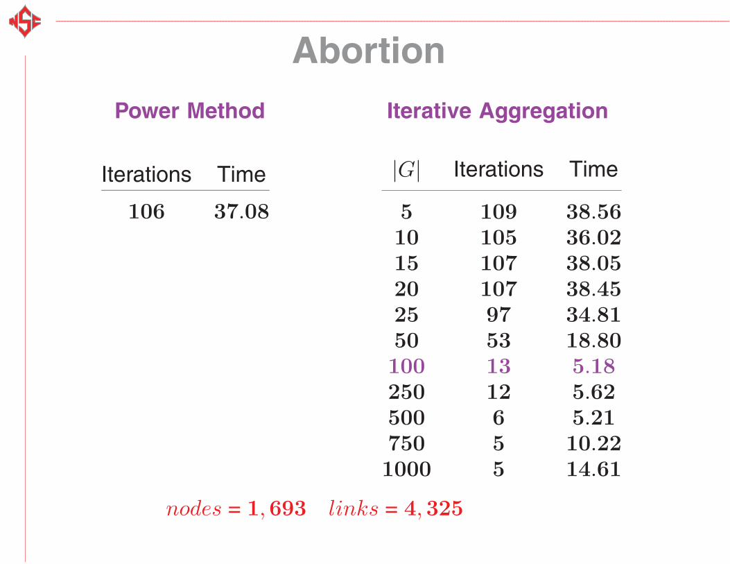
Abortion
Power Method Iterative Aggregation
Iterations Time
106 37.08
|G| Iterations Time
5 109 38.5610 105 36.0215 107 38.0520 107 38.4525 97 34.8150 53 18.80100 13 5.18250 12 5.62500 6 5.21750 5 10.221000 5 14.61
nodes = 1,693 links = 4,325
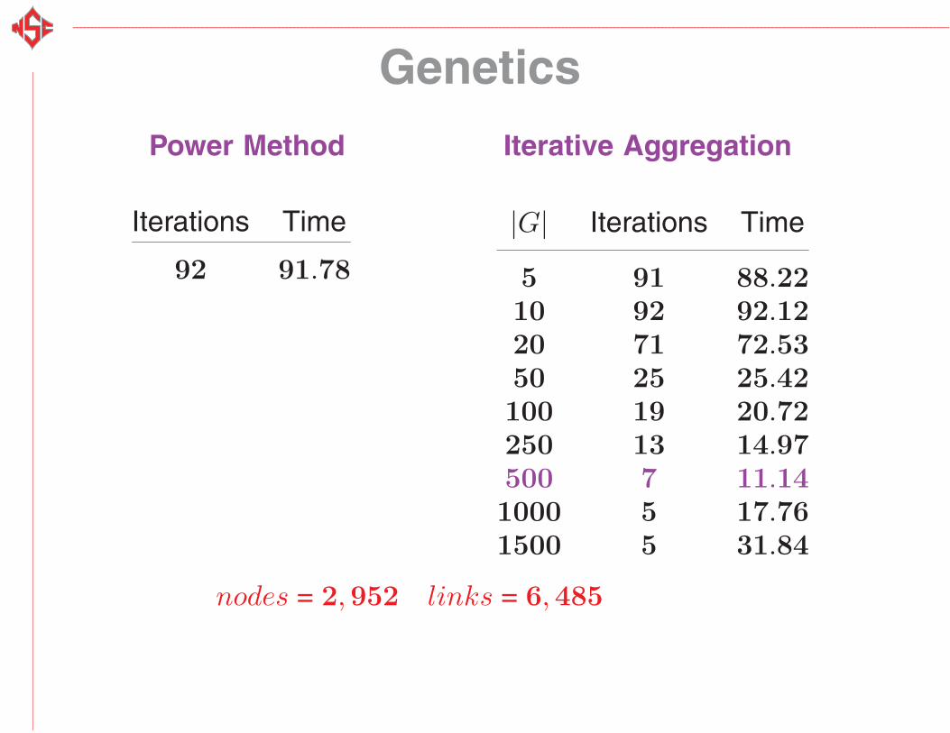
Genetics
Power Method Iterative Aggregation
Iterations Time
92 91.78
|G| Iterations Time
5 91 88.2210 92 92.1220 71 72.5350 25 25.42100 19 20.72250 13 14.97500 7 11.141000 5 17.761500 5 31.84
nodes = 2,952 links = 6,485
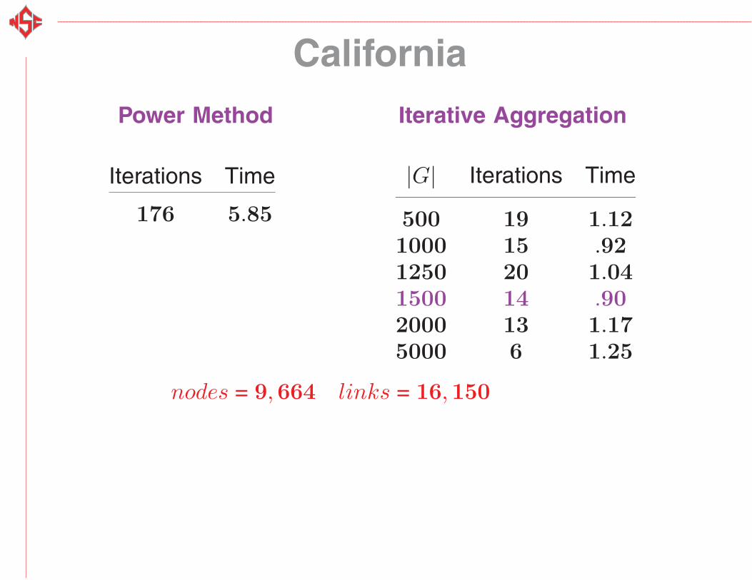
California
Power Method Iterative Aggregation
Iterations Time
176 5.85
|G| Iterations Time
500 19 1.121000 15 .921250 20 1.041500 14 .902000 13 1.175000 6 1.25
nodes = 9,664 links = 16,150

“L” Curves
0 200 400 6000
0.005
0.01
0.015
0.02
0.025
0.03
0.035censorship
0 200 400 6000
0.01
0.02
0.03
0.04movies
0 200 400 6000
0.01
0.02
0.03
0.04
0.05mathworks
0 1000 2000 0 5000 100000
0.005
0.01
0.015
0.02
0.025abortion
0 1000 2000 30000
0.005
0.01
0.015
0.02
0.025
0
0.002
0.004
0.008
0.006
0.01genetics CA
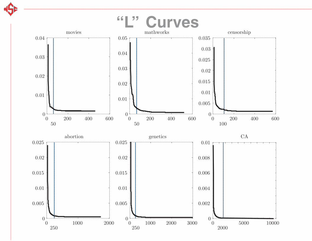
“L” Curves
0 200 400 6000
0.005
0.01
0.015
0.02
0.025
0.03
0.035censorship
1000 200
50400 600
0
0.01
0.02
0.03
0.04movies
500 200 400 600
0
0.01
0.02
0.03
0.04
0.05mathworks
2500 1000 2000
0
0.005
0.01
0.015
0.02
0.025abortion
2500 1000 2000 3000
0
0.005
0.01
0.015
0.02
0.025genetics
20000 5000 10000
0
0.002
0.004
0.008
0.006
0.01CA
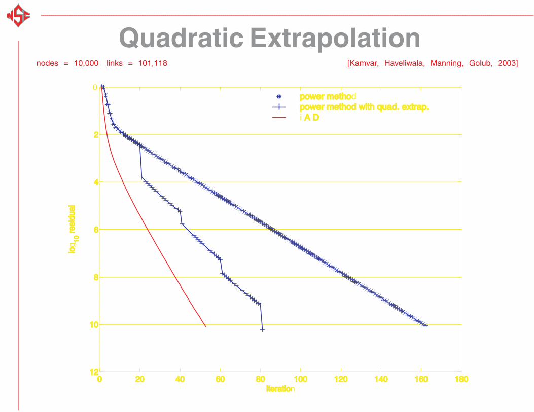
Quadratic Extrapolationnodes = 10,000 links = 101,118 [Kamvar, Haveliwala, Manning, Golub, 2003]
0 20 40 60 80 100 120 140 160 180 12
10 10
8 8
6 6
4 4
2 2
0
iteratioiteration
lolog 1010
res
idua
l r
esid
ual
power methopower methodpower method with quad. extrap.power method with quad. extrap.
Quadratic Extrapolationnodes = 10,000 links = 101,118 [Kamvar, Haveliwala, Manning, Golub, 2003]
0 20 40 60 80 100 120 140 160 180 12
10 10
8 8
6 6
4 4
2 2
0
iteratioiteration
lolog 1010
res
idua
l r
esid
ual
power methopower methodpower method with quad. extrap.power method with quad. extrap.i A D A D
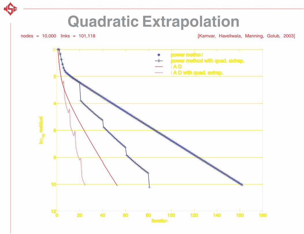
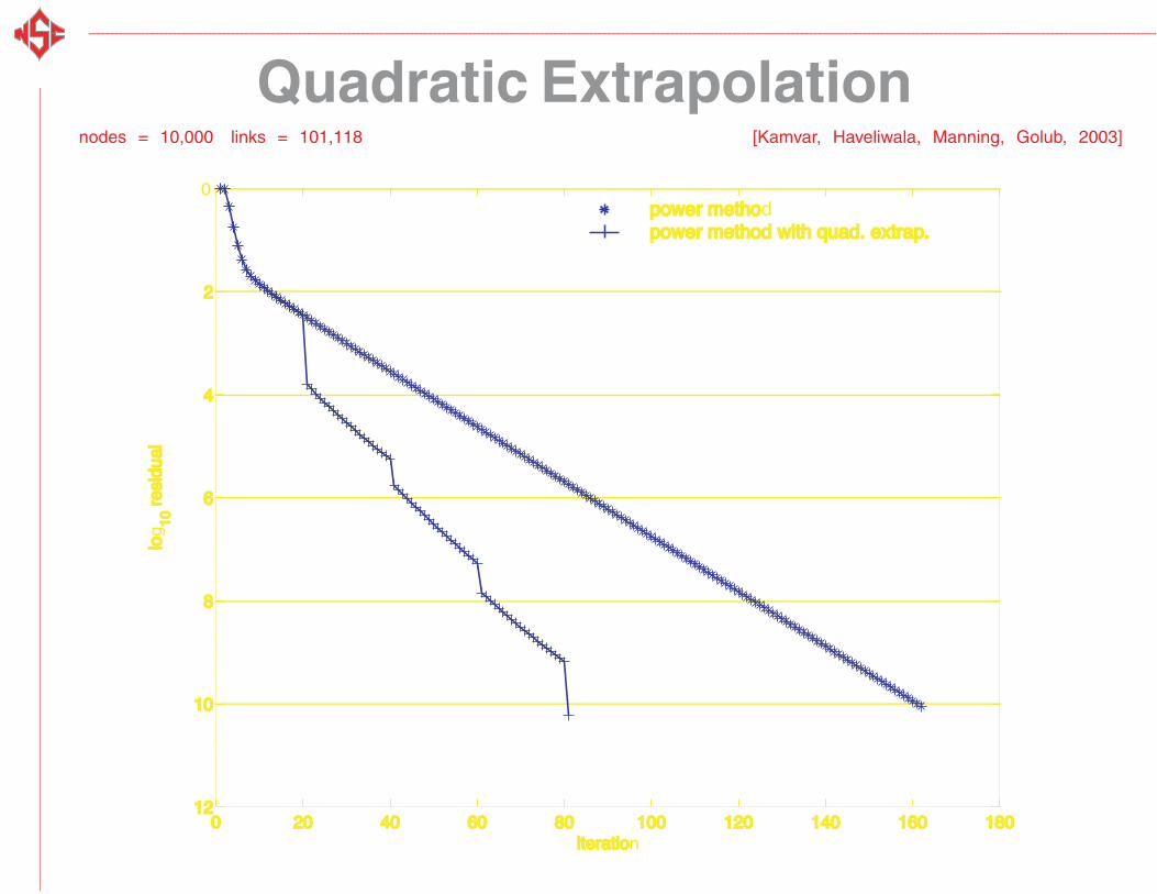
Quadratic Extrapolationnodes = 10,000 links = 101,118 [Kamvar, Haveliwala, Manning, Golub, 2003]
0 20 40 60 80 100 120 140 160 180 12
10 10
8 8
6 6
4 4
2 2
0
iteratioiteration
lolog 1010
res
idua
l r
esid
ual
power methopower methodpower method with quad. extrap.power method with quad. extrap.i A D A Di A D A D with quad. extrap. with quad. extrap.
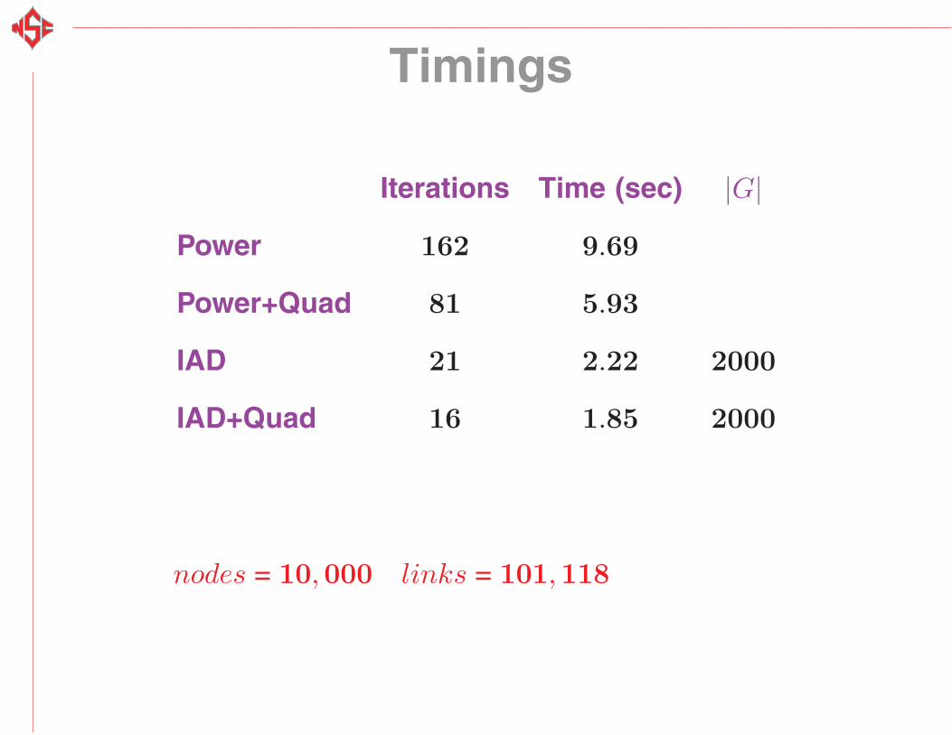
Timings
Iterations Time (sec) |G|
Power 162 9.69
Power+Quad 81 5.93
IAD 21 2.22 2000
IAD+Quad 16 1.85 2000
nodes = 10,000 links = 101,118
Conclusion
Iterative aggregation shows
promise for updating
Markov chains
Especially for those having
power law distributions
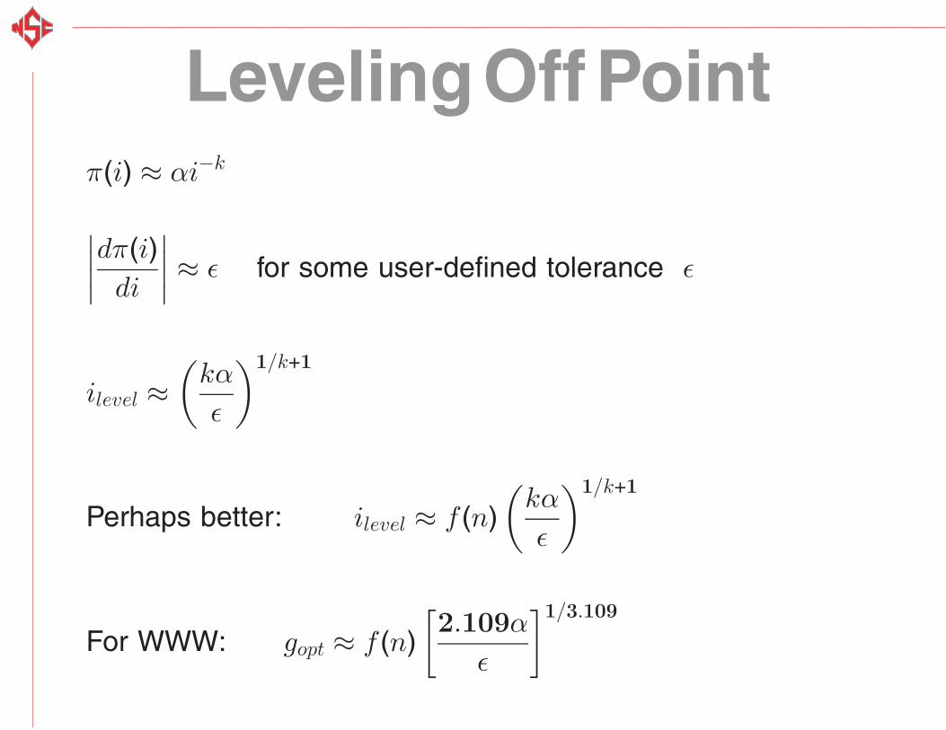
LevelingOffPointπ(i) ≈ αi−k
∣∣∣∣dπ(i)di
∣∣∣∣ ≈ ε for some user-defined tolerance ε
ilevel ≈(
kα
ε
)1/k+1
Perhaps better: ilevel ≈ f (n)(
kα
ε
)1/k+1
For WWW: gopt ≈ f (n)[2.109α
ε
]1/3.109