Phenotypic Plasticity and Maternal Effects Short-term responses to changing climates?
description

Basic Concepts of Plasticity and Mohr Coulomb ModelMohr Coulomb Model
Prof. Minna Karstunen
University of Strathclyde
Basic Concepts of Plasticity
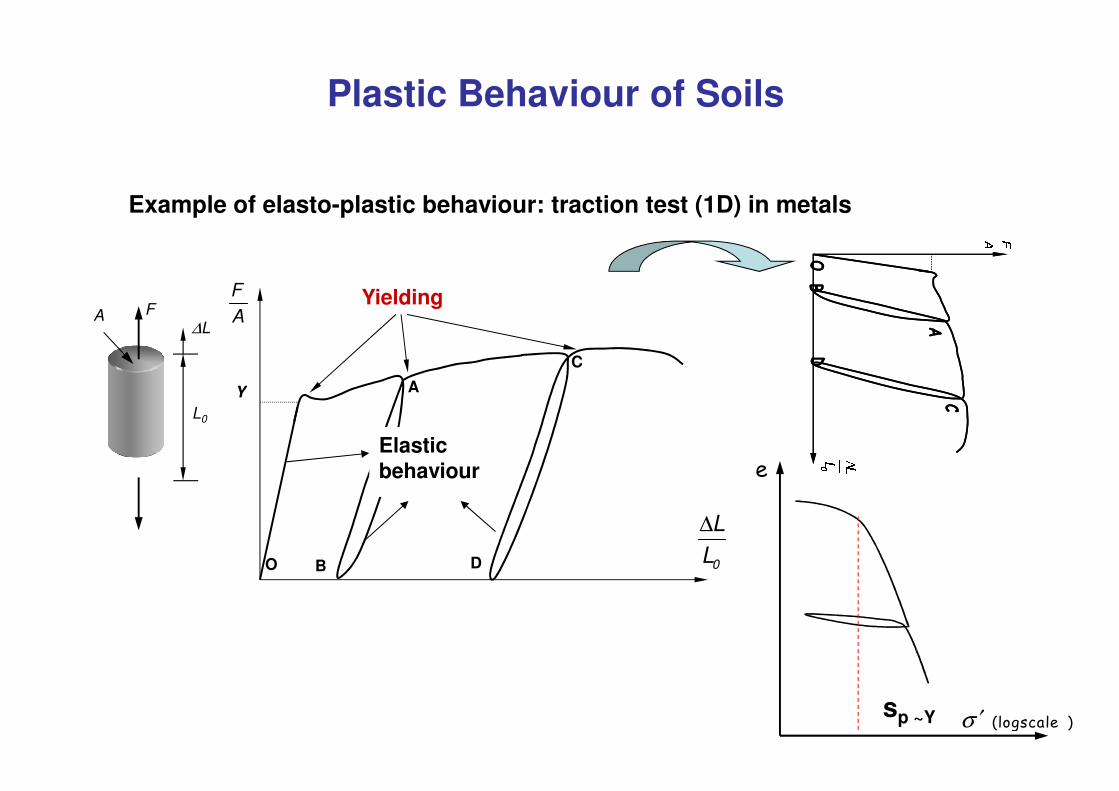
Example of elasto-plastic behaviour: traction test (1D) in metals
YieldingF
AF∆L
A
C
A
Y
B
A
DO
B
A
DO
Plastic Behaviour of Soils
B
A
DO
∆
0
L
L
Y
L0
Elastic behaviour
CC
e
(logscale )σ ′sp ~Y
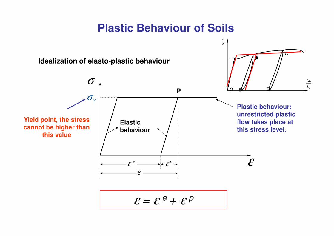
Idealization of elasto-plastic behaviour
Yσ
σP
Yield point, the stress
Plastic behaviour: unrestricted plastic
F
A
B
A
D
C
O
∆
0
L
L
Plastic Behaviour of Soils
εeεpεε
Yield point, the stress cannot be higher than
this value
Elastic behaviour
flow takes place at this stress level.
ε = ε e + ε p
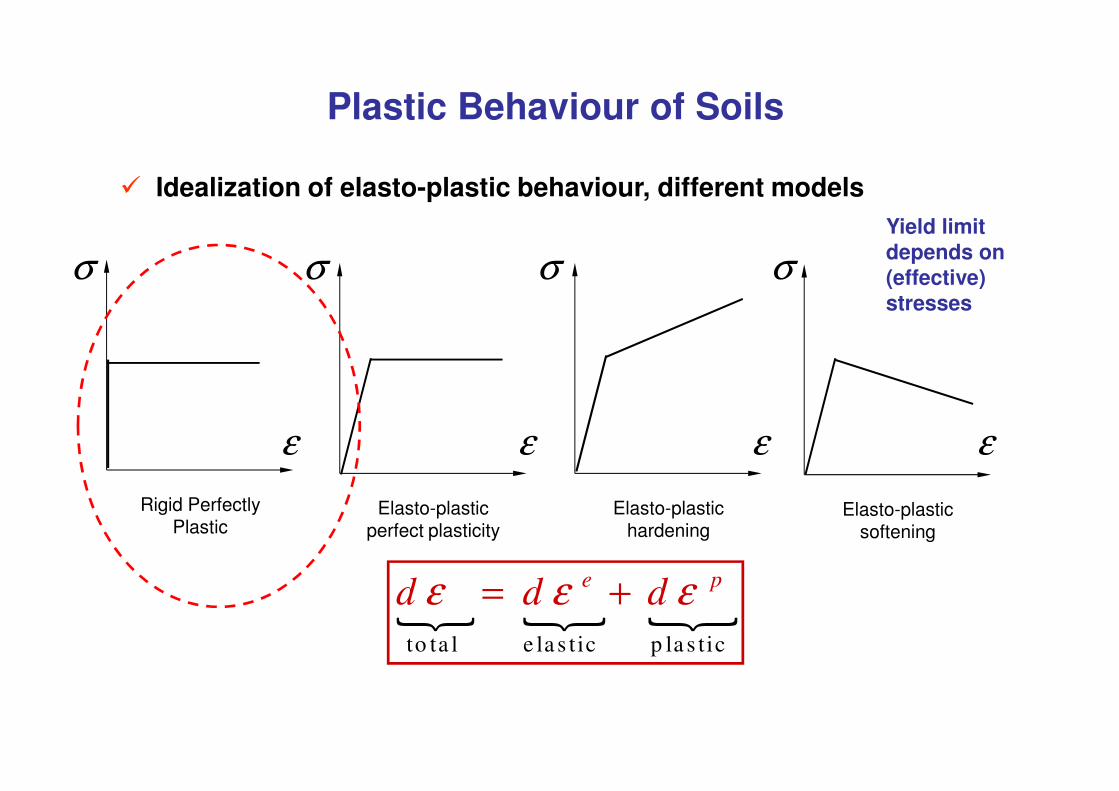
� Idealization of elasto-plastic behaviour, different models
σ σ σ σYield limit depends on (effective) stresses
Plastic Behaviour of Soils
{ { {to ta l e la s t ic p la s tic
ε ε ε= +e pd d d
Rigid PerfectlyPlastic
Elasto-plastic perfect plasticity
Elasto-plastic hardening
Elasto-plasticsoftening
ε ε ε ε
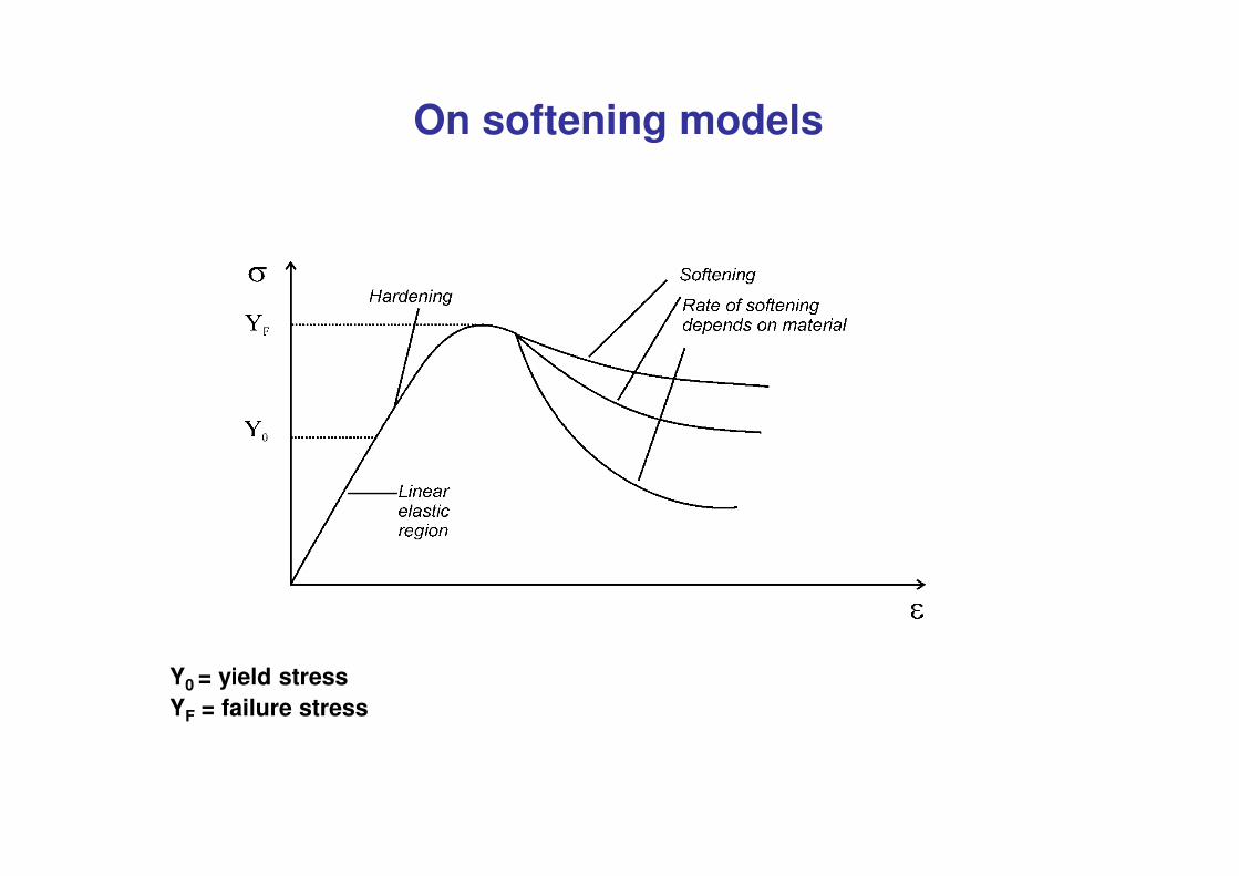
On softening models
Y0 = yield stress
YF = failure stress
� Plastic models allow
� to determine in a direct way the ultimate states and failure
� to model irrecoverable strains
� to model changes in material behaviour
Some Basic Concepts
� to model changes in material behaviour
� to model a more proper way the behaviour of fragile or
quasi-fragile materials
Some Basic Concepts
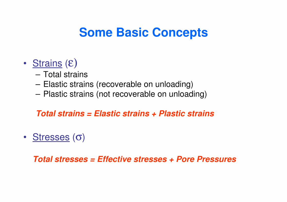
• Strains (ε)– Total strains– Elastic strains (recoverable on unloading) – Plastic strains (not recoverable on unloading)
Total strains = Elastic strains + Plastic strains
• Stresses (σ)
Total stresses = Effective stresses + Pore Pressures
Some Basic Concepts
• Stresses are related to elastic strains even in nonlinear theories
• Stresses are stresses - there is nothing like elastic stress and plastic stress.elastic stress and plastic stress.
• We talk mainly in terms of effective stress.
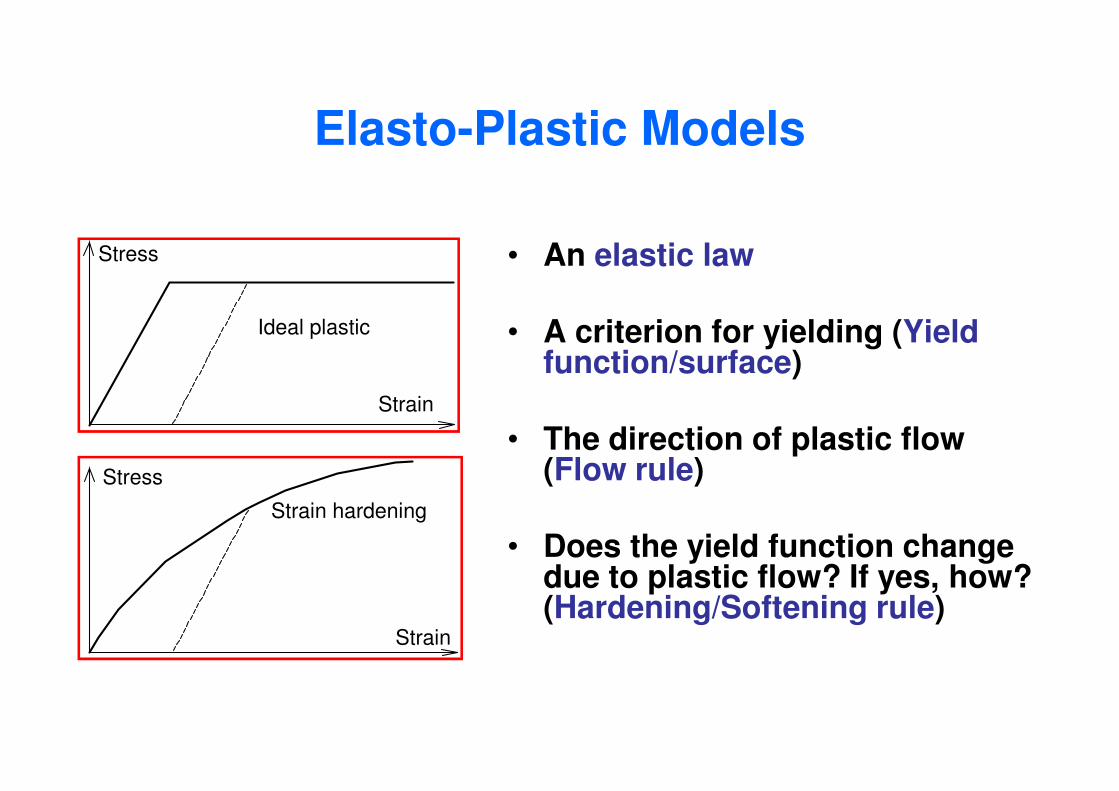
Elasto-Plastic Models
• An elastic law
• A criterion for yielding (Yield function/surface)
Ideal plastic
Stress
Strain
• The direction of plastic flow (Flow rule)
• Does the yield function change due to plastic flow? If yes, how? (Hardening/Softening rule)
Stress
Strain
Strain hardening
Strain
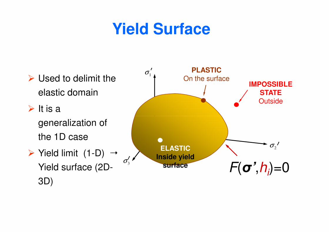
� Used to delimit the
elastic domain
� It is a
PLASTICOn the surface
IMPOSSIBLE STATEOutside
1σ
Yield Surface
generalization of
the 1D case
� Yield limit (1-D) �
Yield surface (2D-
3D)
ELASTICInside yield
surface ( , ) 0ij i
F σ ξ =
2σ
3σ
F(σ’,hi)=0
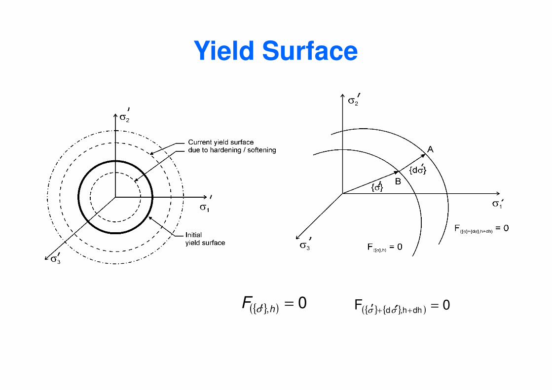
Yield Surface
{ } { }( ) 0F dhh,d =++ σσ{ }( ) 0, =hF σ
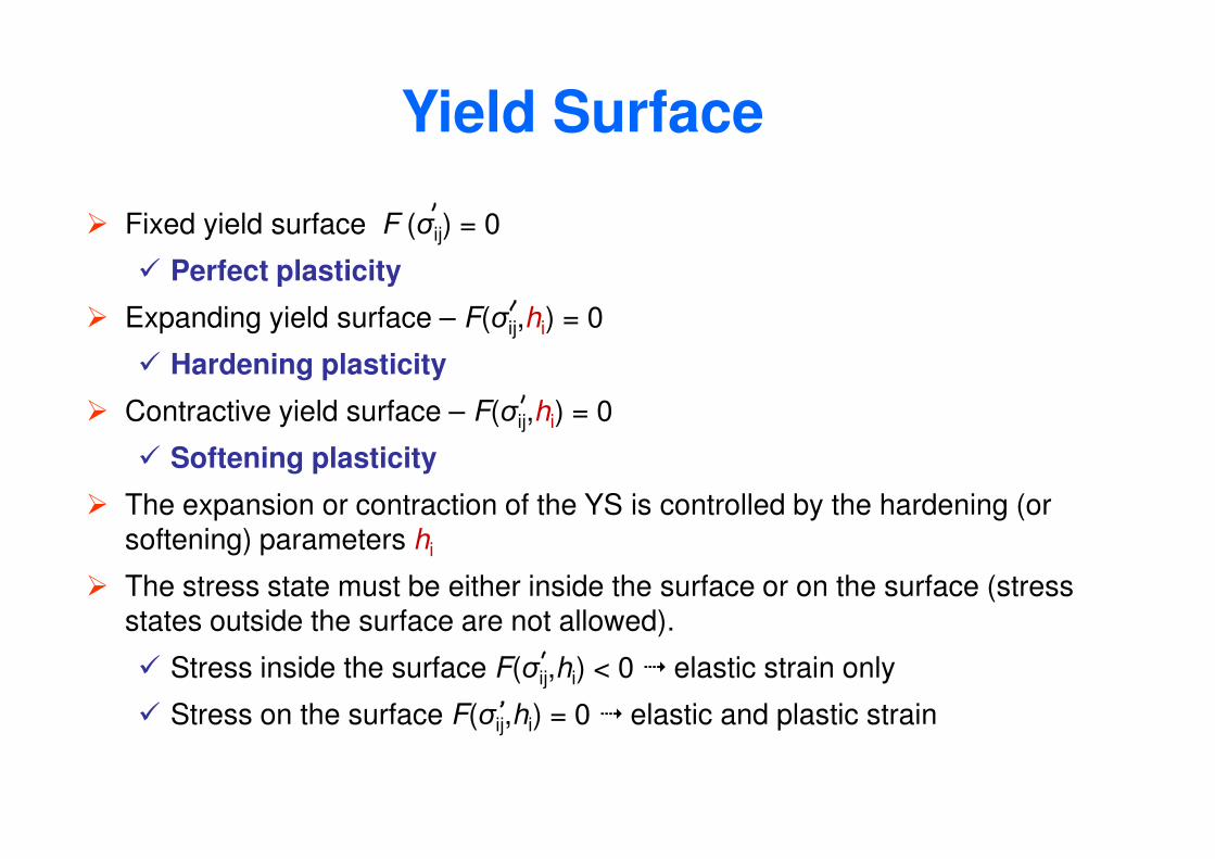
� Fixed yield surface F (σij) = 0
� Perfect plasticity
� Expanding yield surface – F(σij,hi) = 0
� Hardening plasticity
� Contractive yield surface – F(σij,hi) = 0
Yield Surface
ij i
� Softening plasticity
� The expansion or contraction of the YS is controlled by the hardening (or softening) parameters hi
� The stress state must be either inside the surface or on the surface (stress states outside the surface are not allowed).
� Stress inside the surface F(σij,hi) < 0 � elastic strain only
� Stress on the surface F(σij,hi) = 0 � elastic and plastic strain
� The YS is often expressed in term of the stresses or stress invariants.
� p',q are typical stress variables used to describe soil behaviour and, also, to
define the YS
� Therefore typical expression of the YS are as follows:
( ), , 0f p q p′ ′ =
Yield Surface
( ), 0f hσ =
� where is a typical hardening parameter (h) used in geotechnical models.
The hardening parameter(s) control the expansion or contraction of the YS.
( )0, , 0f p q p′ ′ =
0p′
( ), 0ijf hσ =
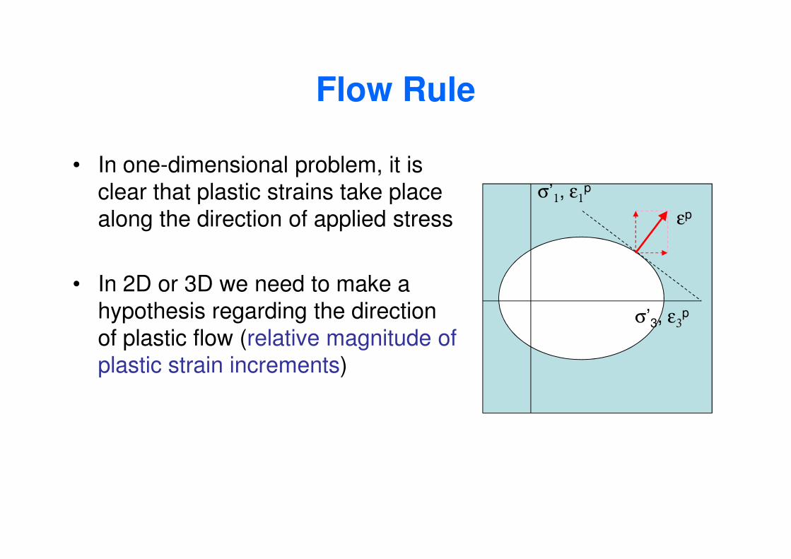
Flow Rule
• In one-dimensional problem, it is clear that plastic strains take place along the direction of applied stress
• In 2D or 3D we need to make a
σ’1, ε1p
εp
• In 2D or 3D we need to make a hypothesis regarding the direction of plastic flow (relative magnitude of plastic strain increments)
σ’3, ε3p
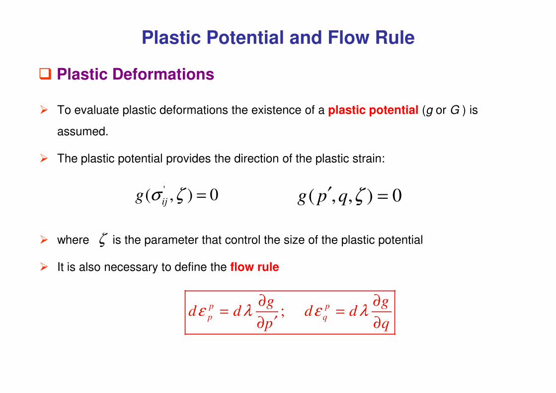
� To evaluate plastic deformations the existence of a plastic potential (g or G ) is
assumed.
� The plastic potential provides the direction of the plastic strain:
0),,( =′ ζqpg
� Plastic Deformations
Plastic Potential and Flow Rule
'( , ) 0ij
g σ ζ =
� where is the parameter that control the size of the plastic potential
� It is also necessary to define the flow rule
ζ
0),,( =′ ζqpg
;p p
p q
g gd d d d
p qε λ ε λ
∂ ∂= =
′∂ ∂
( , ) 0ij
g σ ζ =
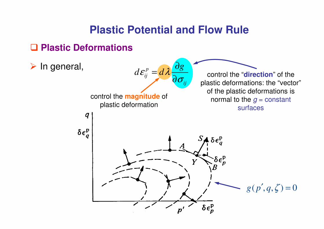
� In general, p
ij
ij
gd dε λ
σ
∂=
∂
control the magnitude of plastic deformation
control the “direction” of the plastic deformations: the “vector”
of the plastic deformations is normal to the g = constant
surfaces
� Plastic Deformations
Plastic Potential and Flow Rule
( , , ) 0g p q ζ′ =
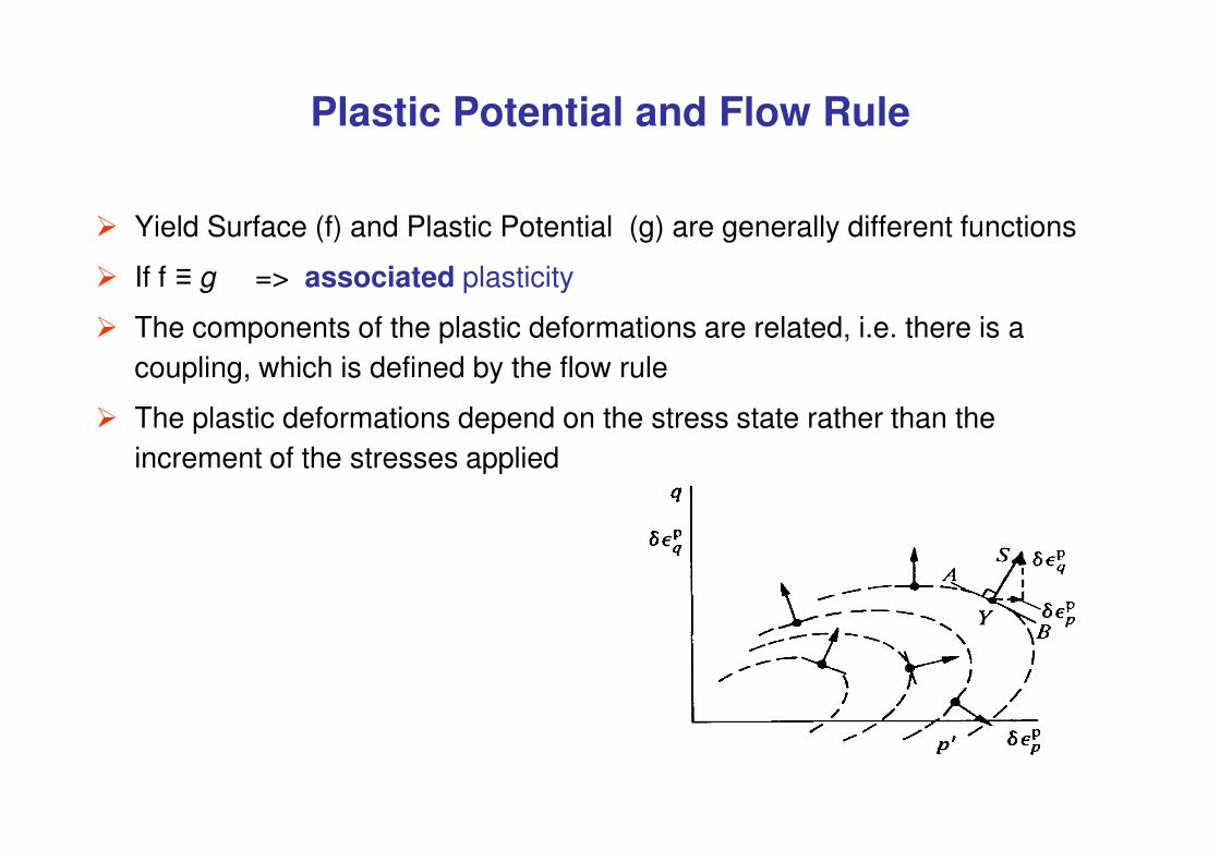
� Yield Surface (f) and Plastic Potential (g) are generally different functions
� If f ≡ g => associated plasticity
� The components of the plastic deformations are related, i.e. there is a
coupling, which is defined by the flow rule
� The plastic deformations depend on the stress state rather than the
Plastic Potential and Flow Rule
� The plastic deformations depend on the stress state rather than the
increment of the stresses applied
Plastic Potential and Flow Rule
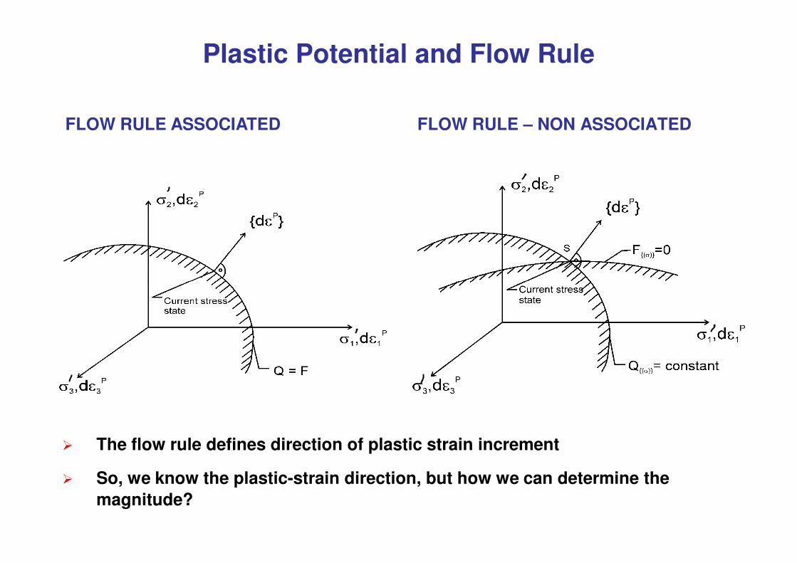
FLOW RULE – NON ASSOCIATEDFLOW RULE ASSOCIATED
� The flow rule defines direction of plastic strain increment
� So, we know the plastic-strain direction, but how we can determine the
magnitude?
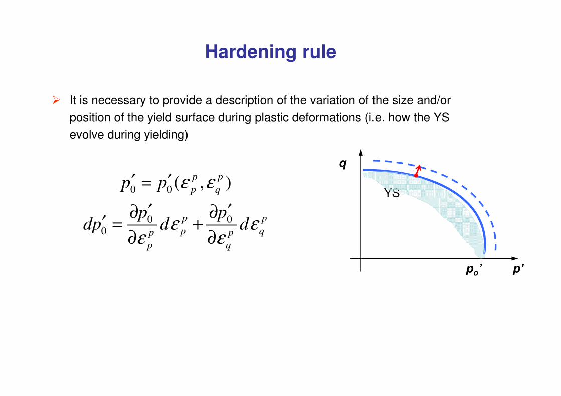
� It is necessary to provide a description of the variation of the size and/or
position of the yield surface during plastic deformations (i.e. how the YS
evolve during yielding)
0 0 ( , )p p
p qp p ε ε′ ′=
Hardening rule
q
YS
0 00
p p
p qp p
p q
p pdp d dε ε
ε ε
′ ′∂ ∂′ = +
∂ ∂
p'po’
YS
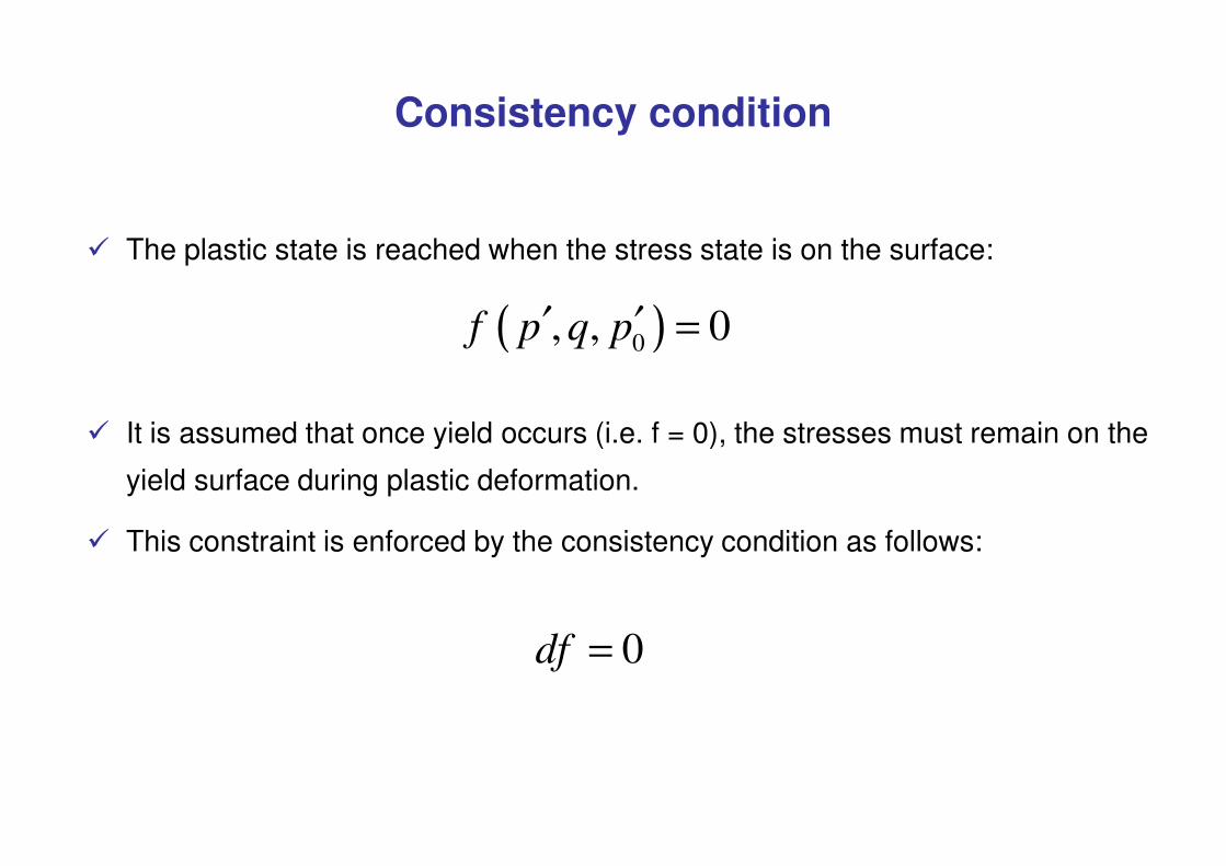
� The plastic state is reached when the stress state is on the surface:
� It is assumed that once yield occurs (i.e. f = 0), the stresses must remain on the
( )0, , 0f p q p′ ′ =
Consistency condition
� It is assumed that once yield occurs (i.e. f = 0), the stresses must remain on the
yield surface during plastic deformation.
� This constraint is enforced by the consistency condition as follows:
0df =
0
0 0 0 0
0 0
0
0
0
p p p p
p q p q
p p
p
p
p
q
f f fdf dp dq
p q p
p p p p
p pf f f g gdf dp dq d d
p q p p q
gd d
gd d
p q
dp
dpε ε ε ε
λ λε ε
λ λε ε
∂ ∂ ∂′= + +
′ ′∂ ∂ ∂
′ ′ ′ ′∂ ∂ ∂ ∂= + = +
∂ ∂ ∂ ∂
′ ′∂ ∂∂ ∂ ∂ ∂ ∂′= + + + =
′ ′ ′∂ ∂ ∂ ∂ ∂ ∂ ∂
∂
′∂
′
′∂
∂
Consistency condition
0
0
0
0
0p p
p q
dp
df dp dq d dp q p p q
f fdp dq
p qd
pf
p
λ λε ε
λ
′
′= + + + = ′ ′ ′∂ ∂ ∂ ∂ ∂ ∂ ∂
∂ ∂′ +
′∂ ∂=
′∂∂−
′∂ ∂
14444244443
0
p p
p q
pg g
p qε ε
′∂∂ ∂+
′∂ ∂ ∂
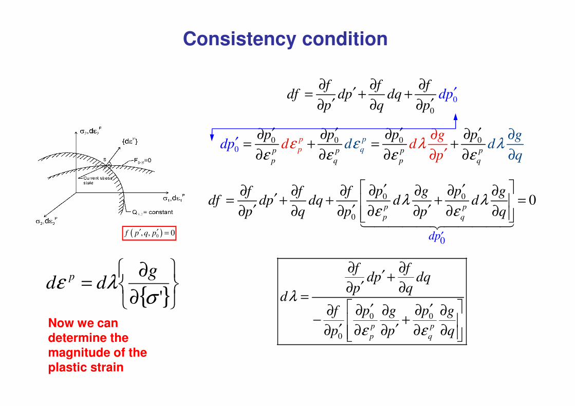
( )0, , 0f p q p′ ′ =
Now we can determine the magnitude of the plastic strain
{ }
∂
∂=
'σλε
gdd p
0 0 0 0
0 0
1
p p p
p
q
p
p
p
p
q p q
p
p
p
f f f fdp dq dp dq
p q p q
p p p pf g g f g g
p p q
gd
p p q
f
d
d p pf g g
g
qpd
ε ε ε ε
ε
ε
εε
∂ ∂ ∂ ∂′ ′+ +
′ ′∂ ∂ ∂ ∂
′ ′ ′ ′∂ ∂ ∂ ∂∂ ∂ ∂ ∂ ∂ ∂− + − +
′ ′ ′ ′∂ ∂ ∂ ∂ ∂ ∂ ∂ ∂ ∂ ∂
∂
−= ′ ′∂ ∂∂ ∂ ∂
∂ ∂=
∂∂=
′
g f g
dpp p q p
f g f g dq
∂ ∂ ∂ ′′ ′ ′∂ ∂ ∂ ∂ ∂ ∂ ∂ ∂
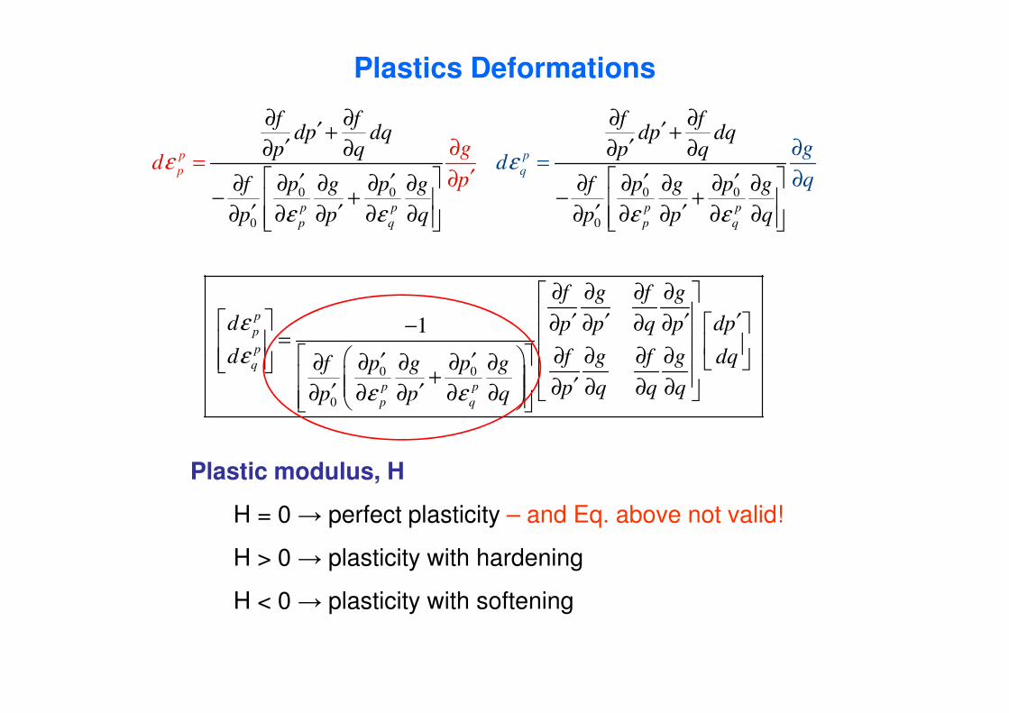
Plastics Deformations
0 0
0
q
p p
p q
d p pf g g
p p q
ε
εε
′ ′∂ ∂∂ ∂ ∂ + ′ ′∂ ∂ ∂ ∂ ∂
f g f g dq
p q q q
∂ ∂ ∂ ∂ ′∂ ∂ ∂ ∂
Plastic modulus, H
H = 0 → perfect plasticity – and Eq. above not valid!
H > 0 → plasticity with hardening
H < 0 → plasticity with softening
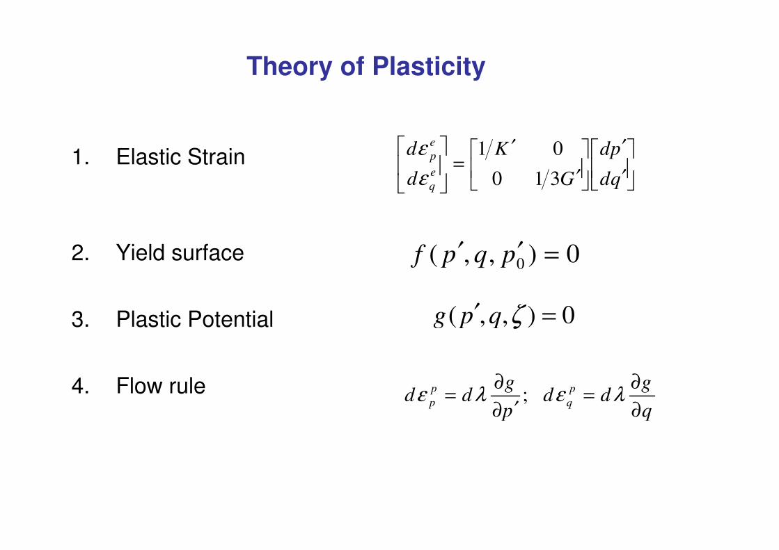
1. Elastic Strain
2. Yield surface
′
′
′
′=
qd
pd
G
K
d
de
q
e
p
310
01
ε
ε
0),,( 0 =′′ pqpf
Theory of Plasticity
3. Plastic Potential
4. Flow rule
0),,( =′ ζqpg
;p p
p q
g gd d d d
p qε λ ε λ
∂ ∂= =
′∂ ∂
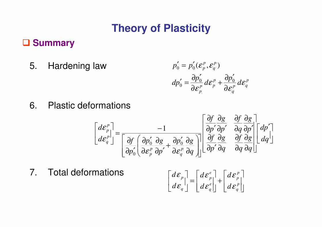
5. Hardening law
6. Plastic deformations
p
qp
q
p
pp
p
p
q
p
p
dp
dp
pd
pp
εε
εε
εε
∂
′∂+
∂
′∂=′
′=′
000
00 ),(
� Summary
Theory of Plasticity
7. Total deformations
′
∂
∂
∂
∂
∂
∂
′∂
∂′∂
∂
∂
∂
′∂
∂
′∂
∂
∂
∂
∂
′∂+
′∂
∂
∂
′∂
′∂
∂
−=
dq
pd
q
g
q
f
q
g
p
f
p
g
q
f
p
g
p
f
q
gp
p
gp
p
fd
d
p
q
p
p
p
q
p
p
εε
ε
ε
00
0
1
e pp p p
e pq q q
d d d
d d d
ε ε ε
ε ε ε
= +
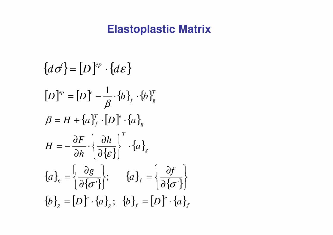
Elastoplastic Matrix
{ } [ ] { }εσ dDdep
⋅=
[ ] [ ] { } { }
{ } [ ] { }eT
T
gf
eep
aDaH
bbDD
⋅⋅+=
⋅⋅−=1
β
β
{ } [ ] { }
{ }{ }
{ }{ }
{ }{ }
{ } [ ] { } { } [ ] { }f
e
fg
e
g
fg
g
T
g
eT
f
aDbaDb
fa
ga
ah
h
FH
aDaH
⋅=⋅=
∂
∂=
∂
∂=
⋅
∂
∂⋅
∂
∂−=
⋅⋅+=
;
';
' σσ
ε
β
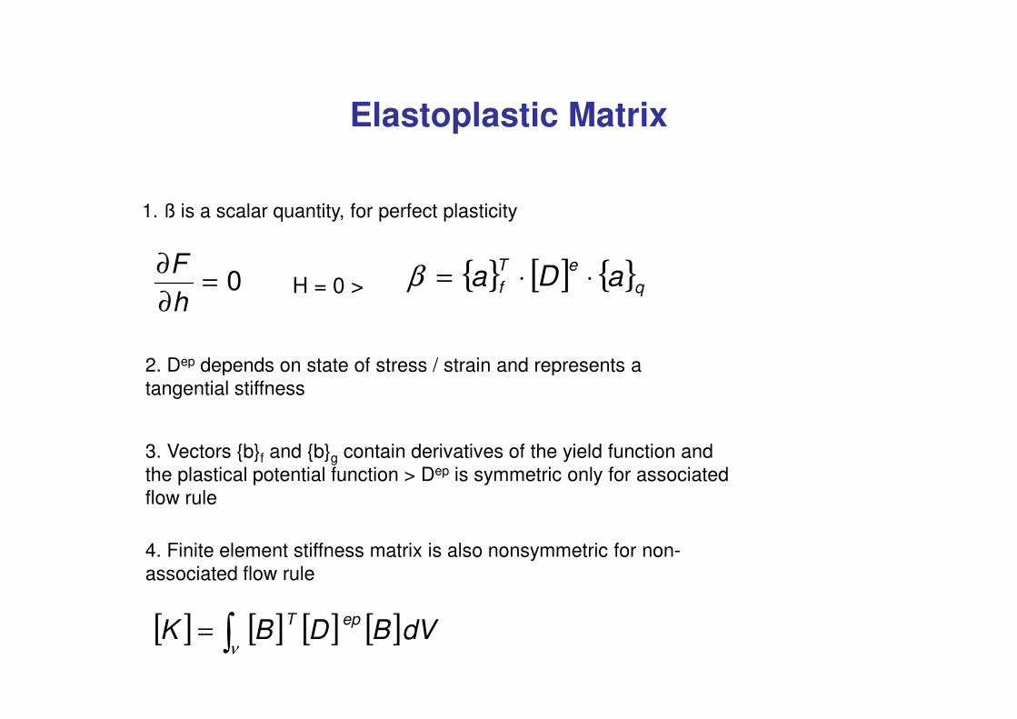
Elastoplastic Matrix
0=∂
∂
h
F { } [ ] { }q
eT
f aDa ⋅⋅=β
1. ß is a scalar quantity, for perfect plasticity
H = 0 >
2. Dep depends on state of stress / strain and represents a
[ ] [ ] [ ] [ ]∫=ν
dVBDBKepT
2. Dep depends on state of stress / strain and represents a tangential stiffness
3. Vectors {b}f and {b}g contain derivatives of the yield function and the plastical potential function > Dep is symmetric only for associated flow rule
4. Finite element stiffness matrix is also nonsymmetric for non-associated flow rule

Mohr Coulomb Model
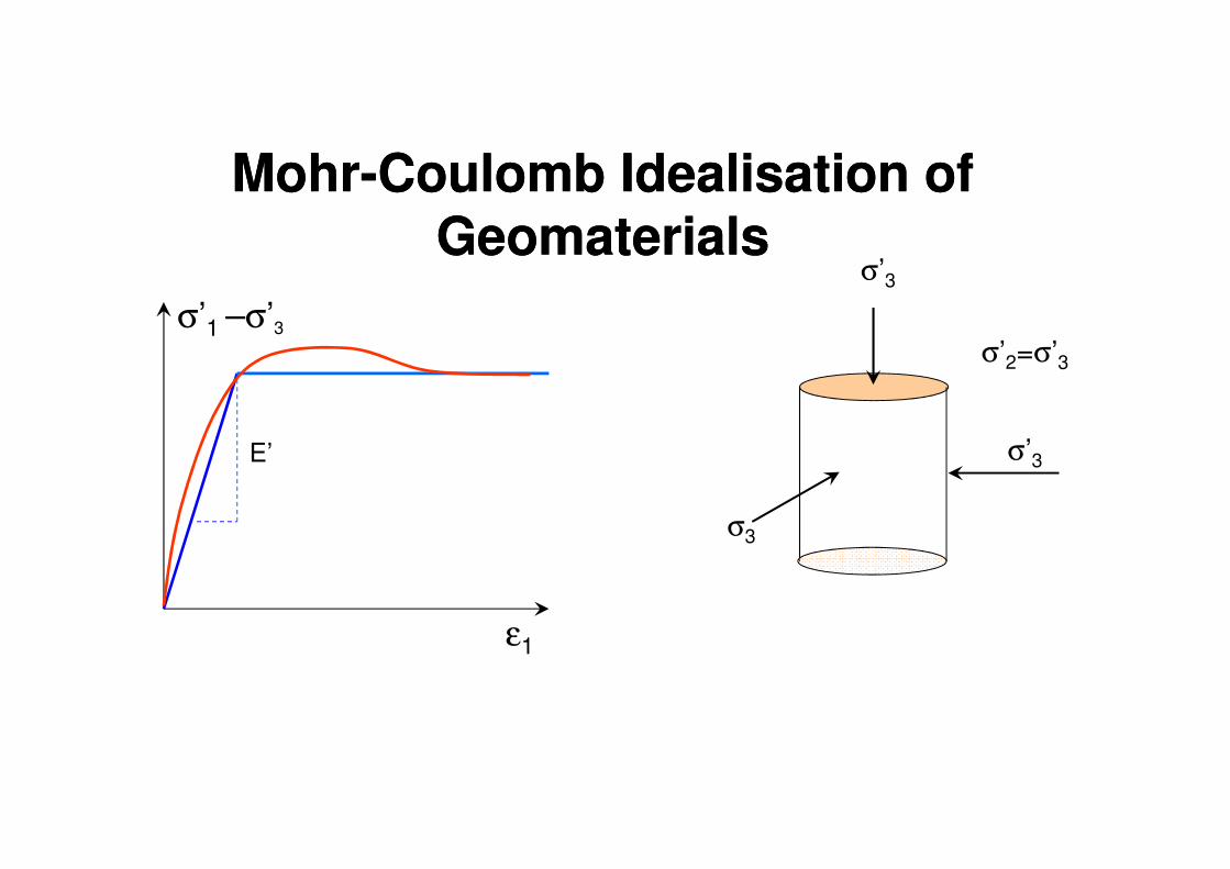
MohrMohr--Coulomb Idealisation of Coulomb Idealisation of GeomaterialsGeomaterials
σ’1 –σ’3
σ’3
σ’2=σ’3
σ’
ε1
σ’3
σ3
E’
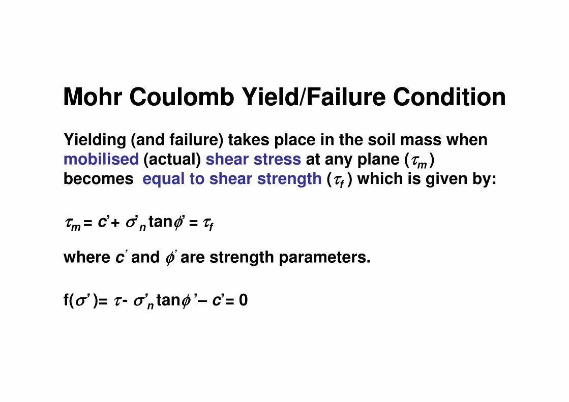
Mohr Coulomb Yield/Failure ConditionMohr Coulomb Yield/Failure Condition
Yielding (and failure) takes place in the soil mass when mobilised (actual) shear stress at any plane (ττττm )becomes equal to shear strength (ττττf ) which is given by:
ττττm = c’+ σσσσ’n tanφφφφ’ = ττττf
where c’ and φφφφ’ are strength parameters.
f(σσσσ’ )= ττττ - σσσσ’n tanφφφφ ’– c’= 0
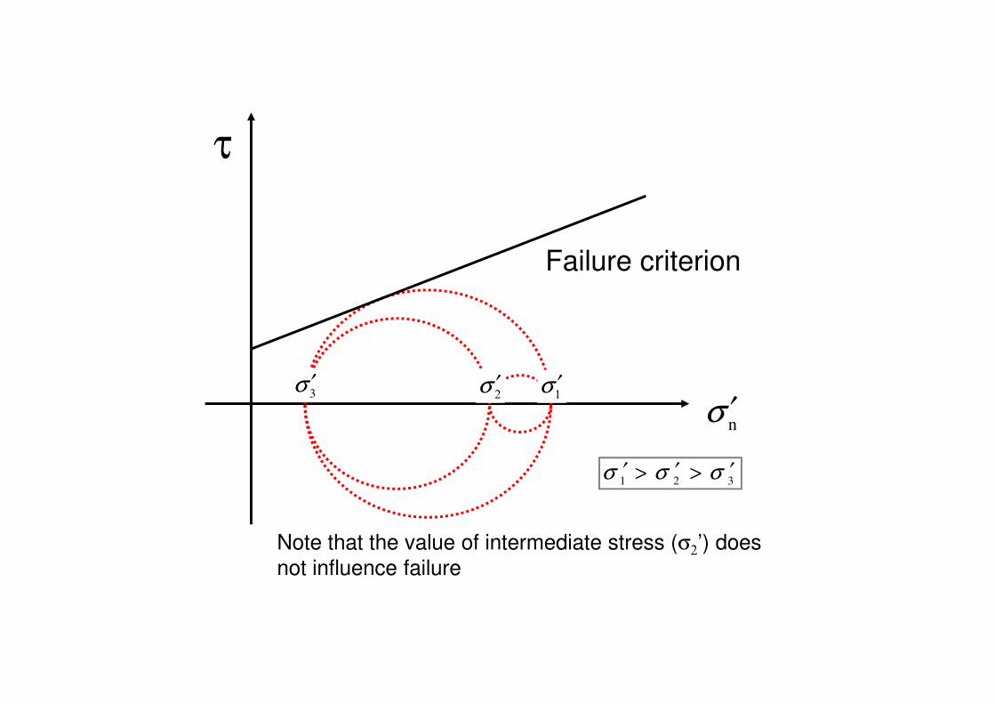
τ
Failure criterion
nσ ′
1σ ′
3σ ′
2σ ′
1 2 3σ σ σ′ ′ ′> >
Note that the value of intermediate stress (σ2’) does not influence failure
σ ′
φ ′
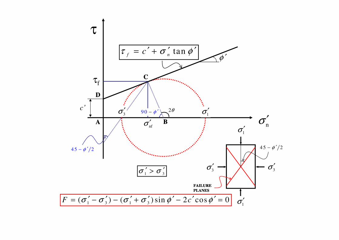
τ
τf
1σ ′3σ ′
AA BB
CC
DD
σ ′
9 0 φ ′− 2θ
tanf n
cτ σ φ′ ′ ′= +
c’
nσ ′AA BB
nfσ ′
4 5 2φ ′−
1 3σ σ′ ′>
4 5 2φ ′−
1σ ′
3σ ′3σ ′
1σ ′
FAILUREFAILURE
PLANESPLANES
1 3 1 3( ) ( ) sin 2 cos 0F cσ σ σ σ φ φ′ ′ ′ ′ ′ ′ ′= − − + − =
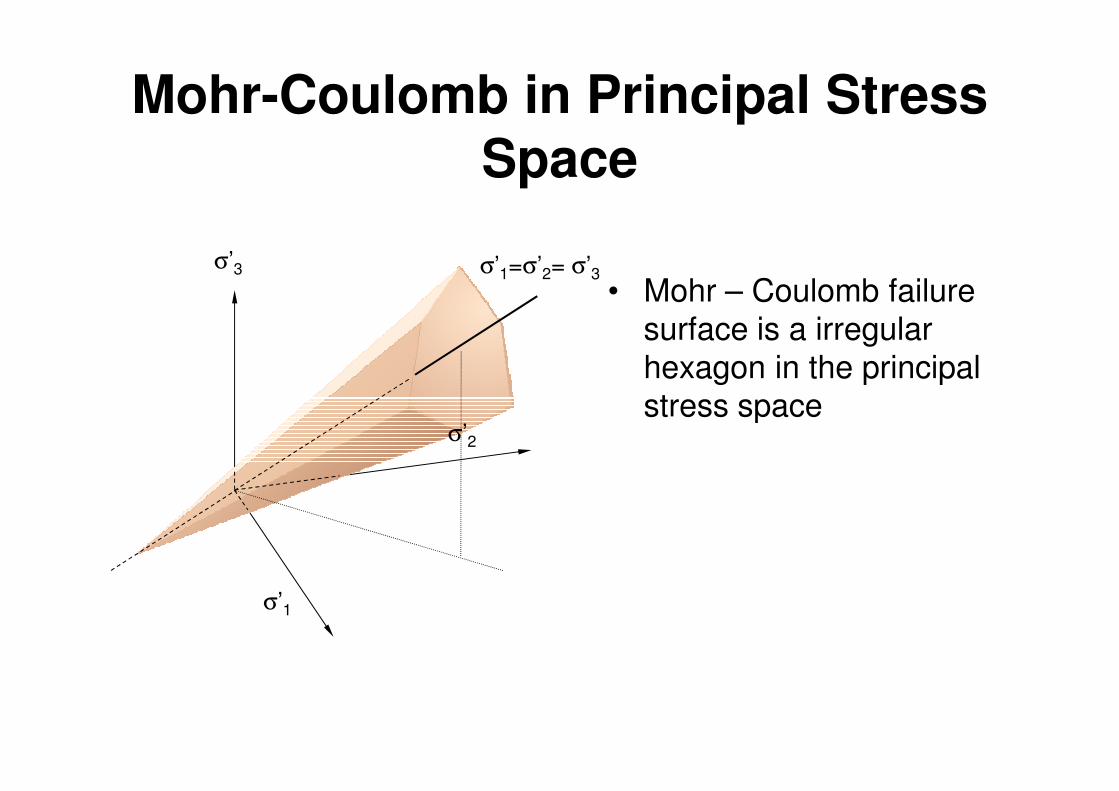
Mohr-Coulomb in Principal Stress Space
• Mohr – Coulomb failure surface is a irregular hexagon in the principal stress space
σ’3 σ’1=σ’2= σ’3
stress space
σ’1
σ’2
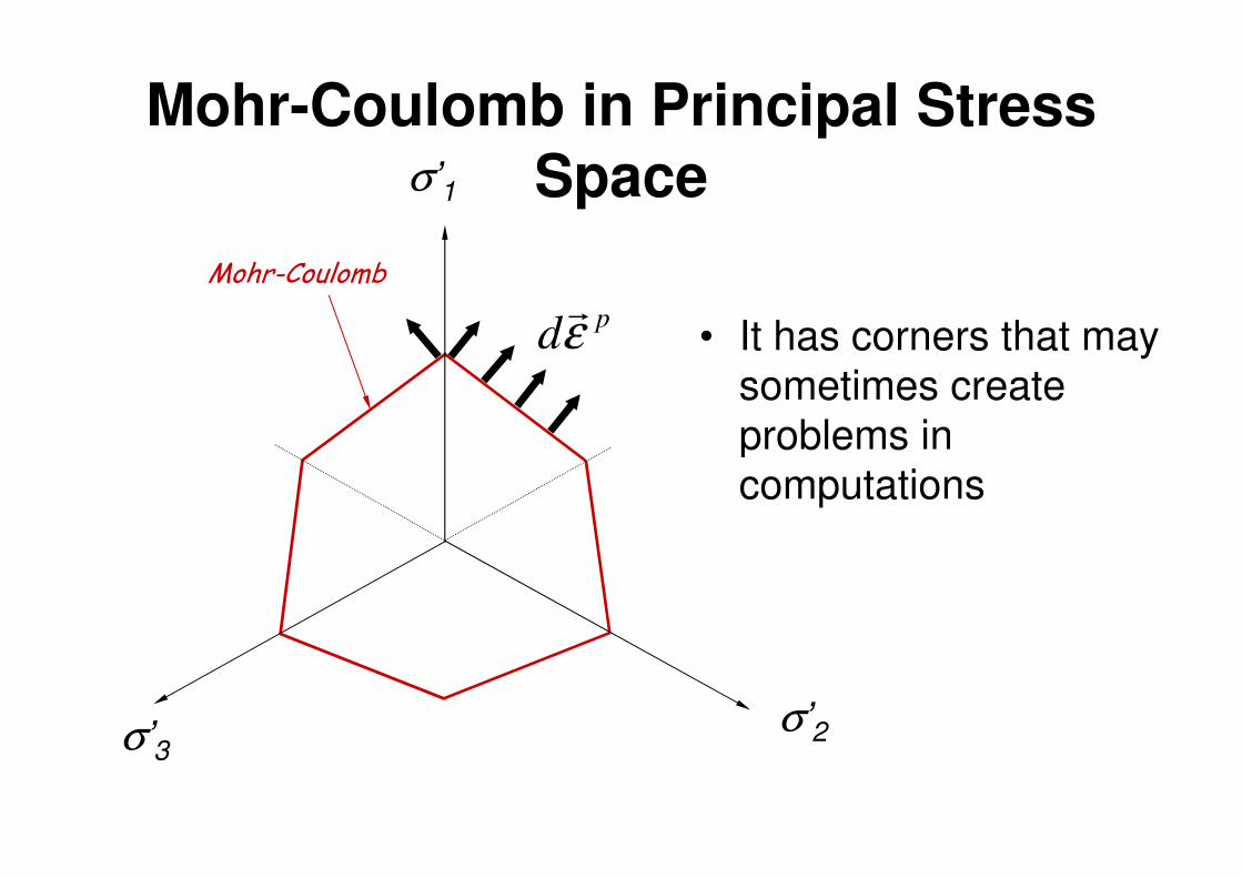
Mohr-Coulomb in Principal Stress Space
• It has corners that may sometimes create problems in
Mohr-Coulomb
pdεr
σ’1
problems in computations
σ’2σ’3
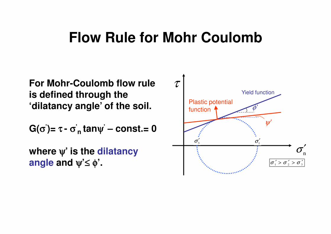
Flow Rule for Mohr Coulomb
For Mohr-Coulomb flow rule is defined through the ‘dilatancy angle’ of the soil.
τYield function
φ’Plastic potential function
G(σσσσ’)= ττττ - σσσσ’n tanψψψψ’ – const.= 0
where ψψψψ’ is the dilatancy angle and ψψψψ’≤≤≤≤ φφφφ’.
nσ ′
1σ ′
3σ ′
1 2 3σ σ σ′ ′ ′> >
ψ’
, τ γ&
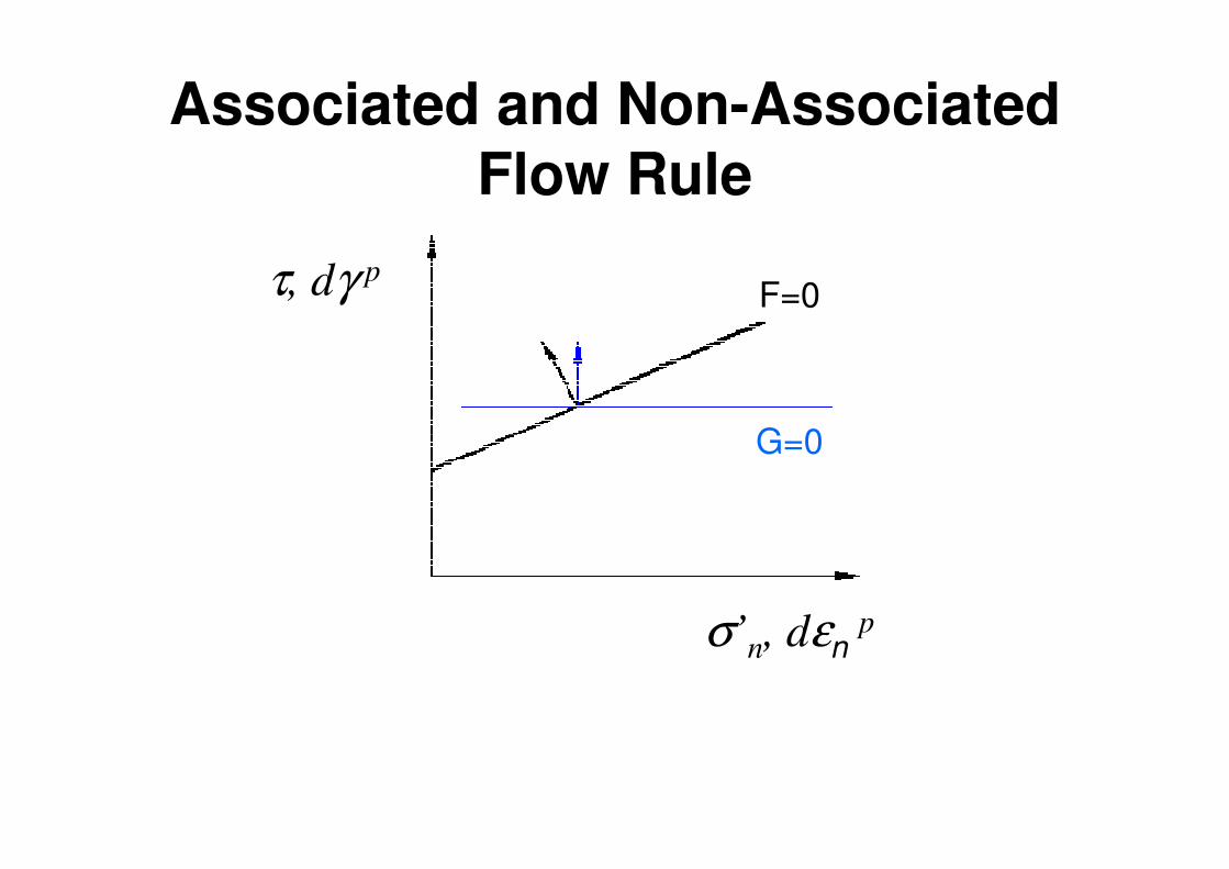
Associated and Non-Associated Flow Rule
τ, dγ p F=0
G=0
, p
n nσ ε′ &σ’n, dεn
p
G=0
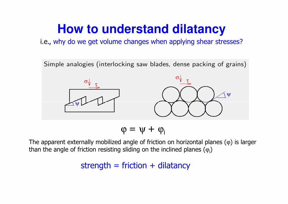
How to understand dilatancyi.e., why do we get volume changes when applying shear stresses?
ϕ = ψ + ϕi
The apparent externally mobilized angle of friction on horizontal planes (ϕ) is larger than the angle of friction resisting sliding on the inclined planes (ϕi)
strength = friction + dilatancy
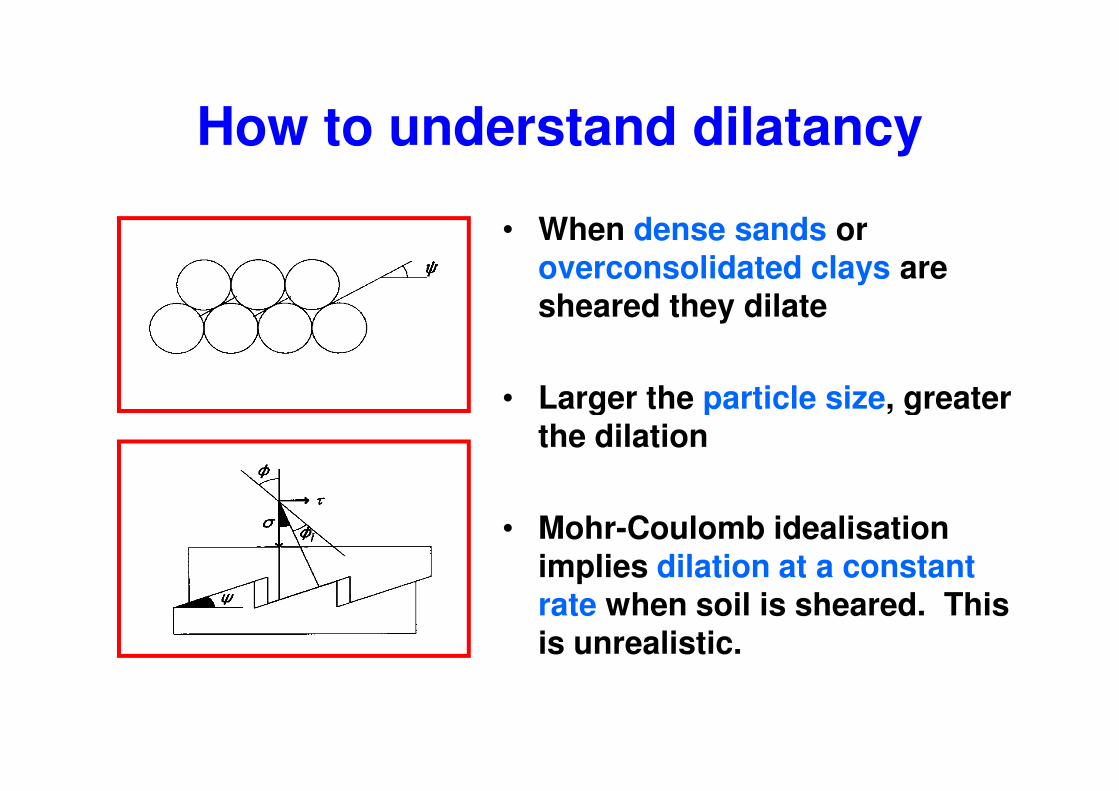
How to understand dilatancy
• When dense sands or overconsolidated clays are sheared they dilate
• Larger the particle size, greater • Larger the particle size, greater the dilation
• Mohr-Coulomb idealisation implies dilation at a constant rate when soil is sheared. This is unrealistic.
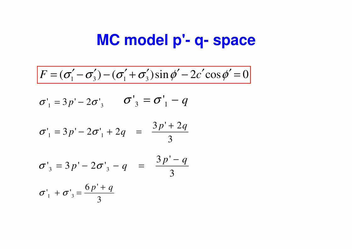
MC model p'- q- space
2'3 qp +
31 '2'3' σσ −= p q−= 13 '' σσ
1 3 1 3( ) ( )sin 2 cos 0F cσ σ σ σ φ φ′ ′ ′ ′ ′ ′ ′= − − + − =
( ) 3131 '''2'3
1' σσσσ −=+= qp 3
2'32'2'3' 11
qpqp
+=+−= σσ
3
'3'2'3' 33
qpqp
−=−−= σσ
3
'6'' 31
qp +=+ σσ
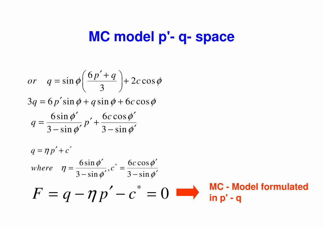
MC model p'- q- space
6sin 2 cos
3
3 6 sin sin 6 cos
p qor q c
q p q c
φ φ
φ φ φ
′ + = +
′= + +
′6sin 6 coscφ φ′ ′
*
*6sin 6 cos,
3 sin 3 sin
q p c
cwhere c
η
φ φη
φ φ
′= +
′ ′= =
′ ′− −
* 0F q p cη ′= − − =MC - Model formulated in p' - q
6sin 6 cos
3 sin 3 sin
cq p
φ φ
φ φ
′ ′′= +
′ ′− −
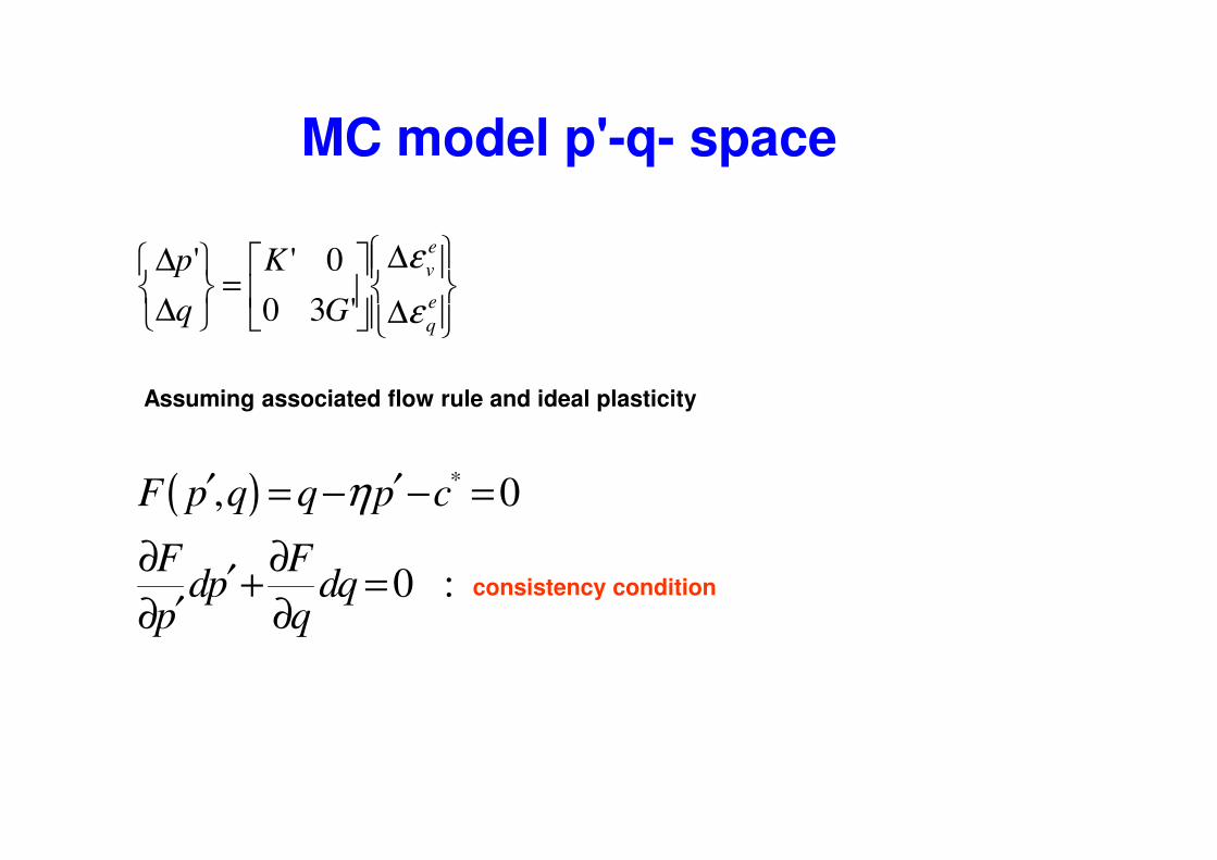
MC model p'-q- space
Assuming associated flow rule and ideal plasticity
∆
∆
=
∆
∆e
q
e
v
G
K
q
p
ε
ε
'30
0''
( )
( )
*, 0
0 :
F p q q p c
F Fdp dq consistency condition
p q
η′ ′= − − =
∂ ∂′+ =
′∂ ∂consistency condition
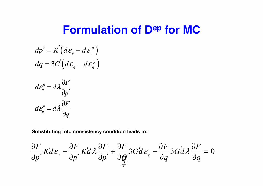
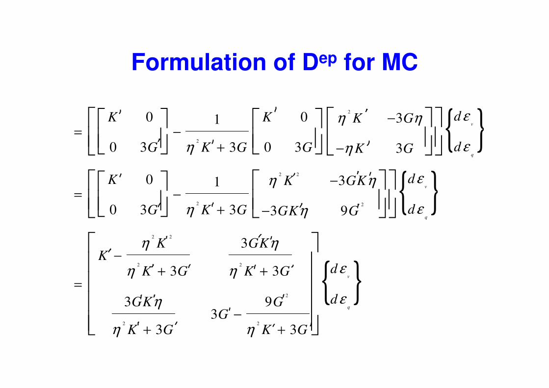
Formulation of Dep for MC
( )
( )3
p
v v
p
q q
dp K d d Hooks law
dq G d d
ε ε
ε ε
′ = −
= −
:p
v
Fd d flowrule
pε λ
∂=
′∂
Substituting into consistency condition leads to:
p
q
p
Fd d
qε λ
′∂
∂=
∂
3 3 0v q
F F F F F FKd Kd Gd Gd
p p p Q q qε λ ε λ
∂ ∂ ∂ ∂ ∂ ∂− + − =
′ ′ ′∂ ∂ ∂ ∂ ∂ ∂
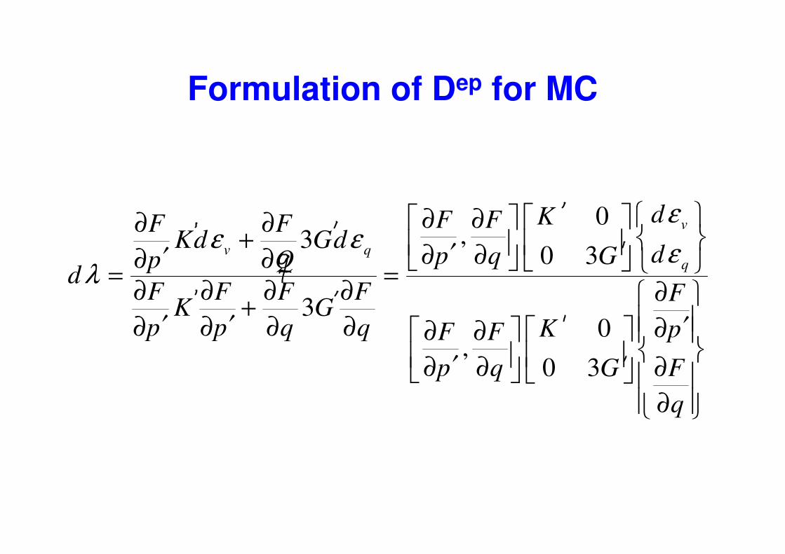
Formulation of Dep for MC
0,3
0 3
v
v qq
dKF FF FKd Gd
dp q Gp Qd
F F F F
εε ε
ελ
∂ ∂ ∂ ∂+ ′∂ ∂′∂ ∂ = =
∂ ∂ ∂ ∂ ∂3
0,
0 3
dF F F F F
K Gp p q q K pF F
p q G F
q
λ = =∂ ∂ ∂ ∂ ∂ +
′ ′ ′∂ ∂ ∂ ∂ ∂ ∂ ∂ ′∂ ∂ ∂ ∂
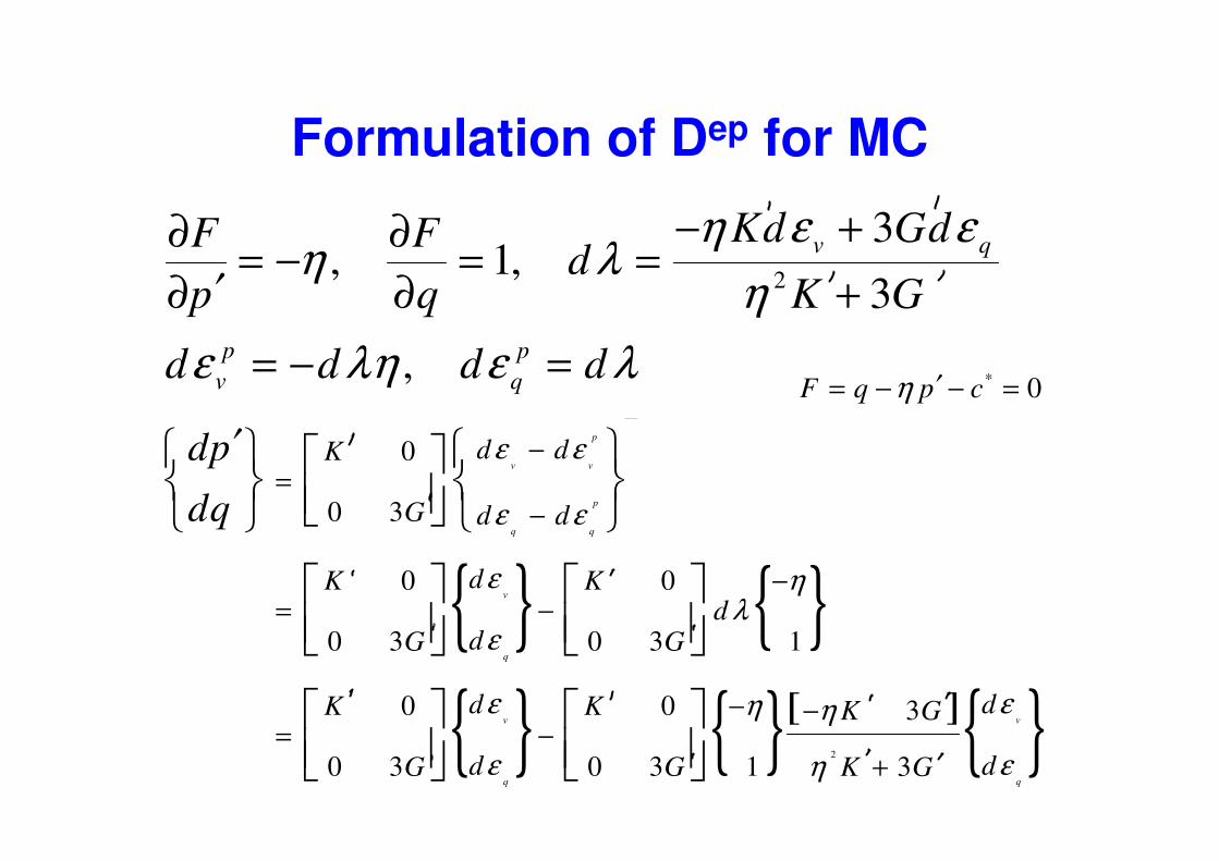
Formulation of Dep for MC
2
3, 1,
3
,
v q
p p
v q
T
Kd GdF Fd
p q K G
d d d d
η ε εη λ
η
ε λη ε λ
− +∂ ∂= − = =
′∂ ∂ +
= − =
dp ε ε−′
* 0F q p cη ′= − − =
{ } { }{ } { }[ ]{ }2
0
0 3
0 0
0 3 0 3 1
0 0 3
0 3 0 3 1 3
p
v v
p
q q
v
q
v v
q q
d dK
G d d
dK Kd
dG G
d dK K K G
d dG G K G
dp
dq
ε ε
ε ε
ε ηλ
ε
ε εη η
ε εη
−=
−
−= −
− −= −
+
′
Formulation of Dep for MC
{ }{ }
2
2
2 2
0 0 31
0 3 0 33 3
0 31
v
q
v
dK K K G
dG GK G K G
dK K GK
εη η
εη η
εη η
−= −
+ −
−= −
{ }
{ }
2 2
2 2
2 2
2
2 2
0 3 3 3 9
3
3 3
3 93
3 3
q
v
q
dG K G GK G
K GKK
dK G K G
dGK GG
K G K G
εη η
η η
εη η
εη
η η
= −+ −
−+ +
=
−+ +
Formulation of Dep for MC
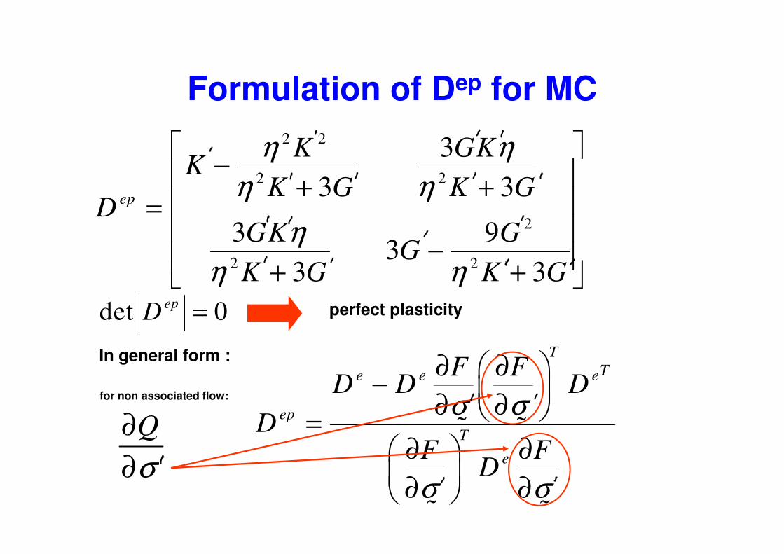
2 2
2 2
2
2 2
3
3 3
3 93
3 3
ep
K GKK
K G K GD
GK GG
K G K G
η η
η η
η
η η
− + +
=
− + + 3 3K G K Gη η+ + det 0ep
D = perfect plasticity
T
Te e e
ep
T
e
F FD D D
DF F
D
σ σ
σ σ
∂ ∂ − ∂ ∂ =
∂ ∂ ∂ ∂
% %
% %
In general form :
for non associated flow:
σ∂
∂Q
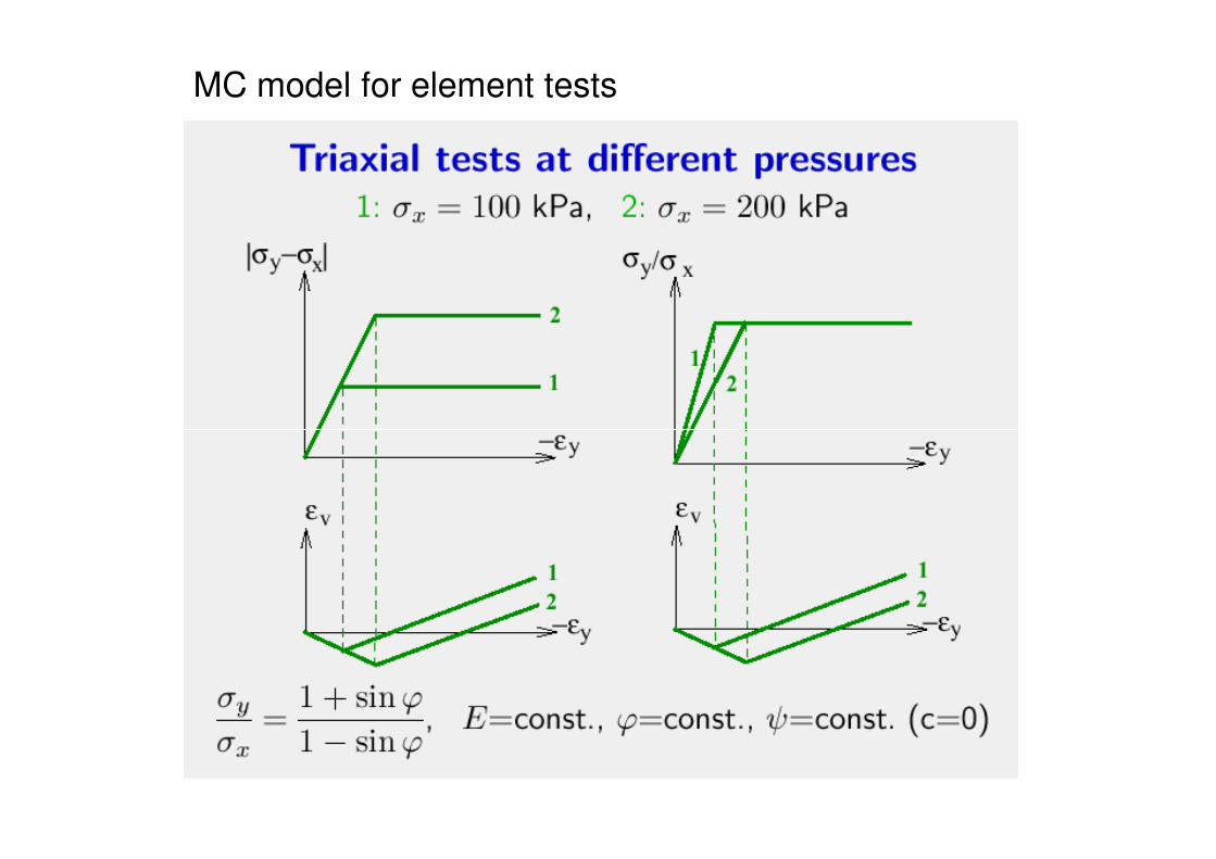
MC model for element tests
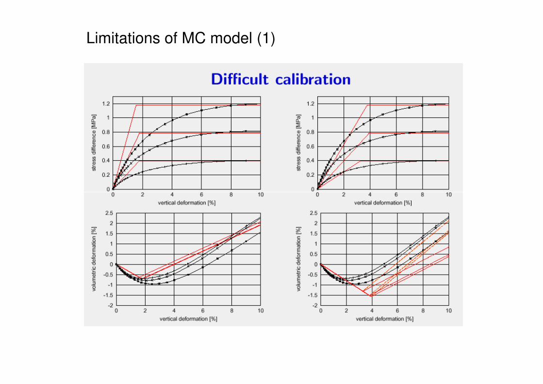
Limitations of MC model (1)
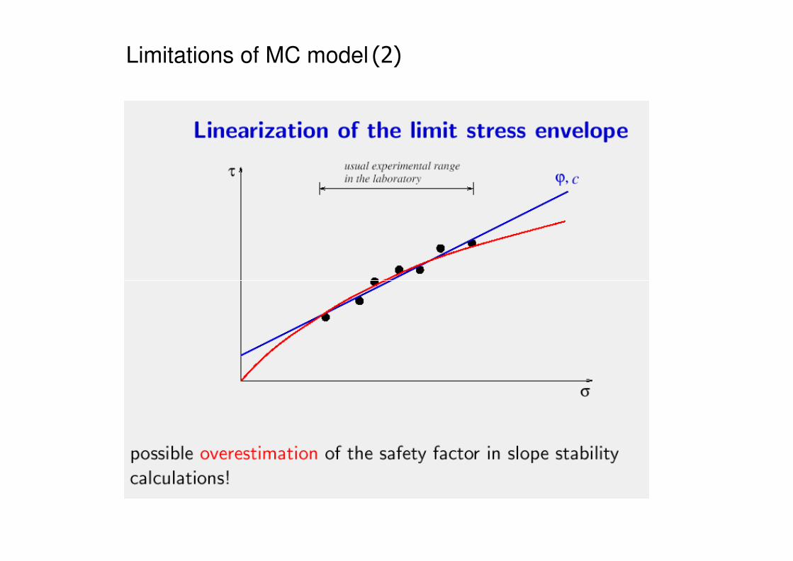
Limitations of MC model (2)
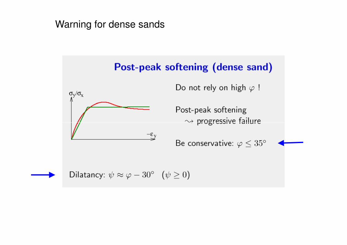
Warning for dense sands
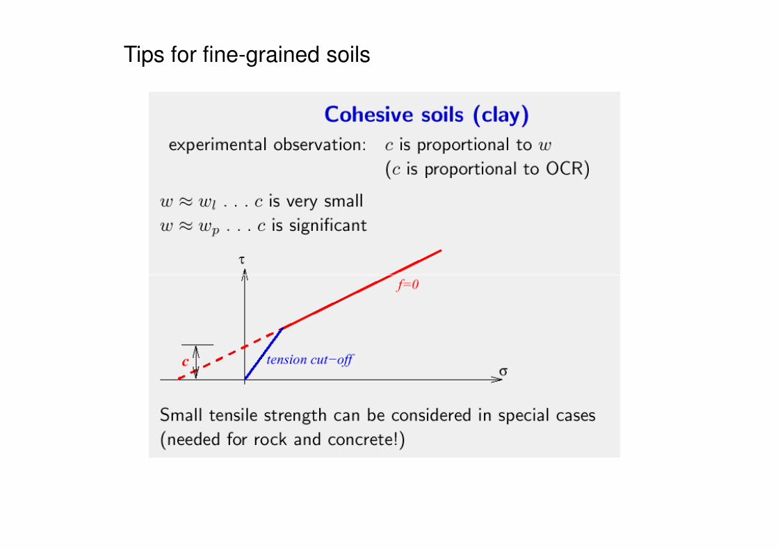
Tips for fine-grained soils
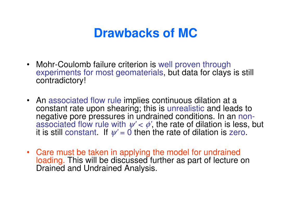
Drawbacks of MC
• Mohr-Coulomb failure criterion is well proven through experiments for most geomaterials, but data for clays is still contradictory!
• An associated flow rule implies continuous dilation at a • An associated flow rule implies continuous dilation at a constant rate upon shearing; this is unrealistic and leads to negative pore pressures in undrained conditions. In an non-associated flow rule with ψ’ < φ’, the rate of dilation is less, but it is still constant. If ψ’ = 0 then the rate of dilation is zero.
• Care must be taken in applying the model for undrained loading. This will be discussed further as part of lecture on Drained and Undrained Analysis.
Drawbacks of MC
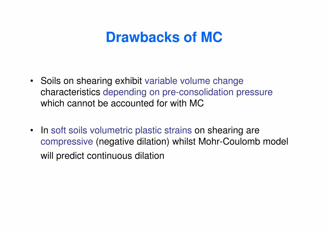
• Soils on shearing exhibit variable volume changecharacteristics depending on pre-consolidation pressurewhich cannot be accounted for with MC
• In soft soils volumetric plastic strains on shearing are compressive (negative dilation) whilst Mohr-Coulomb model
will predict continuous dilation
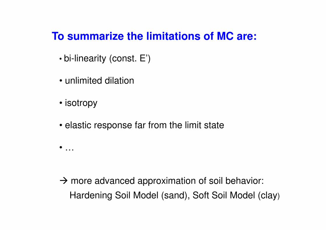
To summarize the limitations of MC are:
• bi-linearity (const. E’)
• unlimited dilation
• isotropy
• elastic response far from the limit state
• …
� more advanced approximation of soil behavior:
Hardening Soil Model (sand), Soft Soil Model (clay)
Other elastic-perfectly plastic modelsmodels
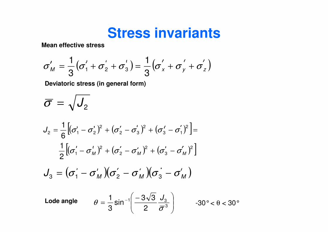
Stress invariants
( ) ( )zyxM σσσσσσσ ++=++=3
1
3
1321
2J=σ
Mean effective stress
Deviatoric stress (in general form)
( ) ( ) ( )[ ]
( ) ( ) ( )[ ]2
3
2
2
2
1
2
13
2
32
2
212
2
1
6
1
MMM
J
σσσσσσ
σσσσσσ
−+−+−
=−+−+−=
( )( )( )MMMJ σσσσσσ −−−= 3213
−= −
3
31
2
33sin
3
1
σθ
JLode angle -30°< θ < 30°
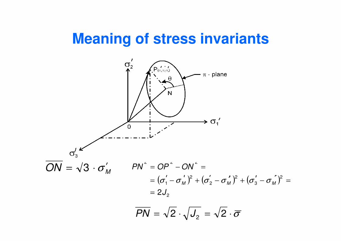
Meaning of stress invariants
σ⋅=⋅= 22 2JPN
( ) ( ) ( )
2
2
3
2
2
2
1
222
2J
ONOPPN
MMM
=
=−+−+−=
=−=
σσσσσσMON σ⋅= 3
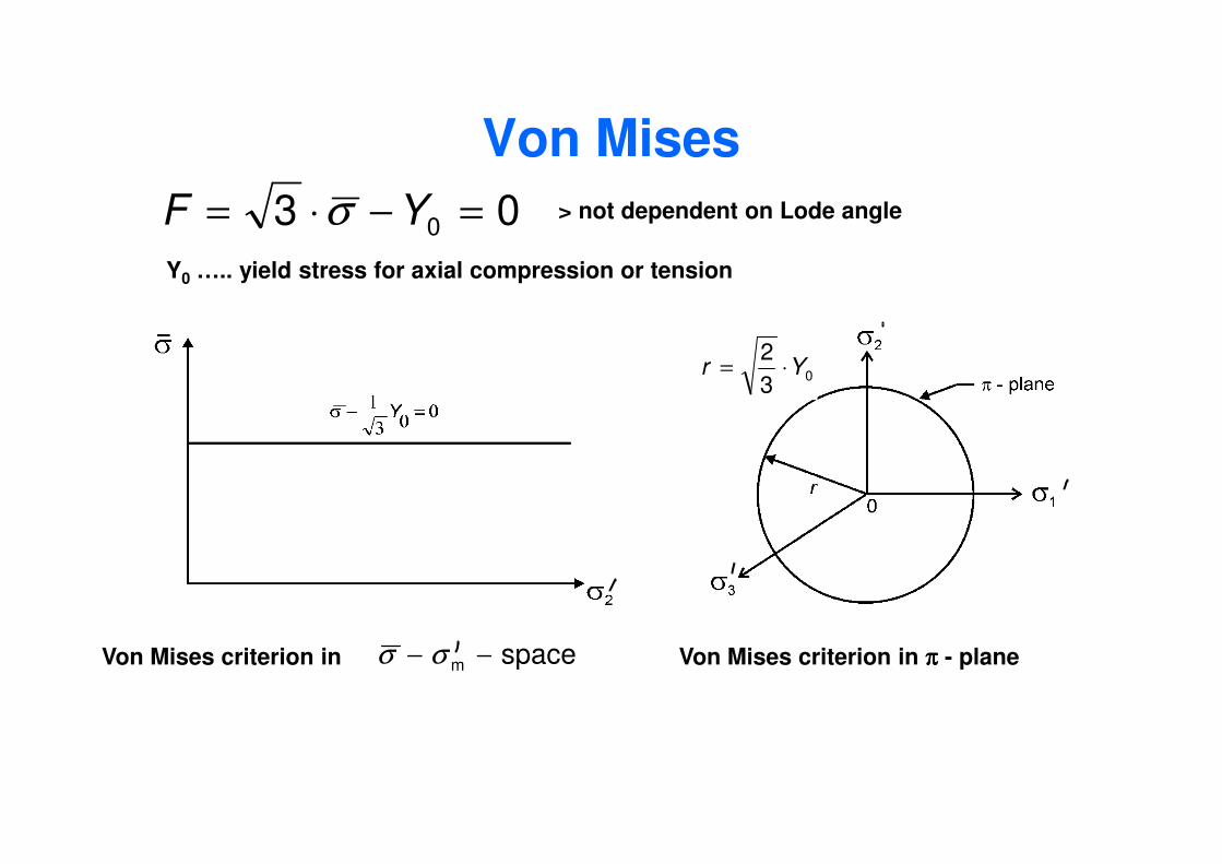
Von Mises
03 0 =−⋅= YF σY0 ….. yield stress for axial compression or tension
> not dependent on Lode angle
03
2Yr ⋅=
Von Mises criterion in spacem −− σσ Von Mises criterion in ππππ - plane
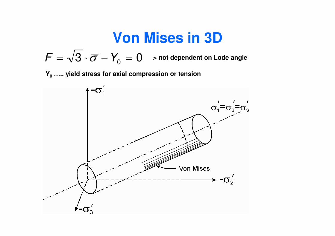
Von Mises in 3D
03 0 =−⋅= YF σY0 ….. yield stress for axial compression or tension
> not dependent on Lode angle
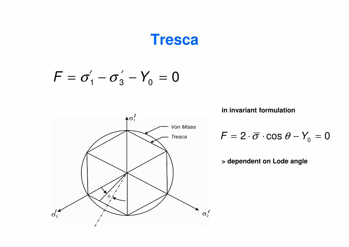
Tresca
0031 =−−= YF σσ
in invariant formulation
0cos2 0 =−⋅⋅= YF θσ
> dependent on Lode angle
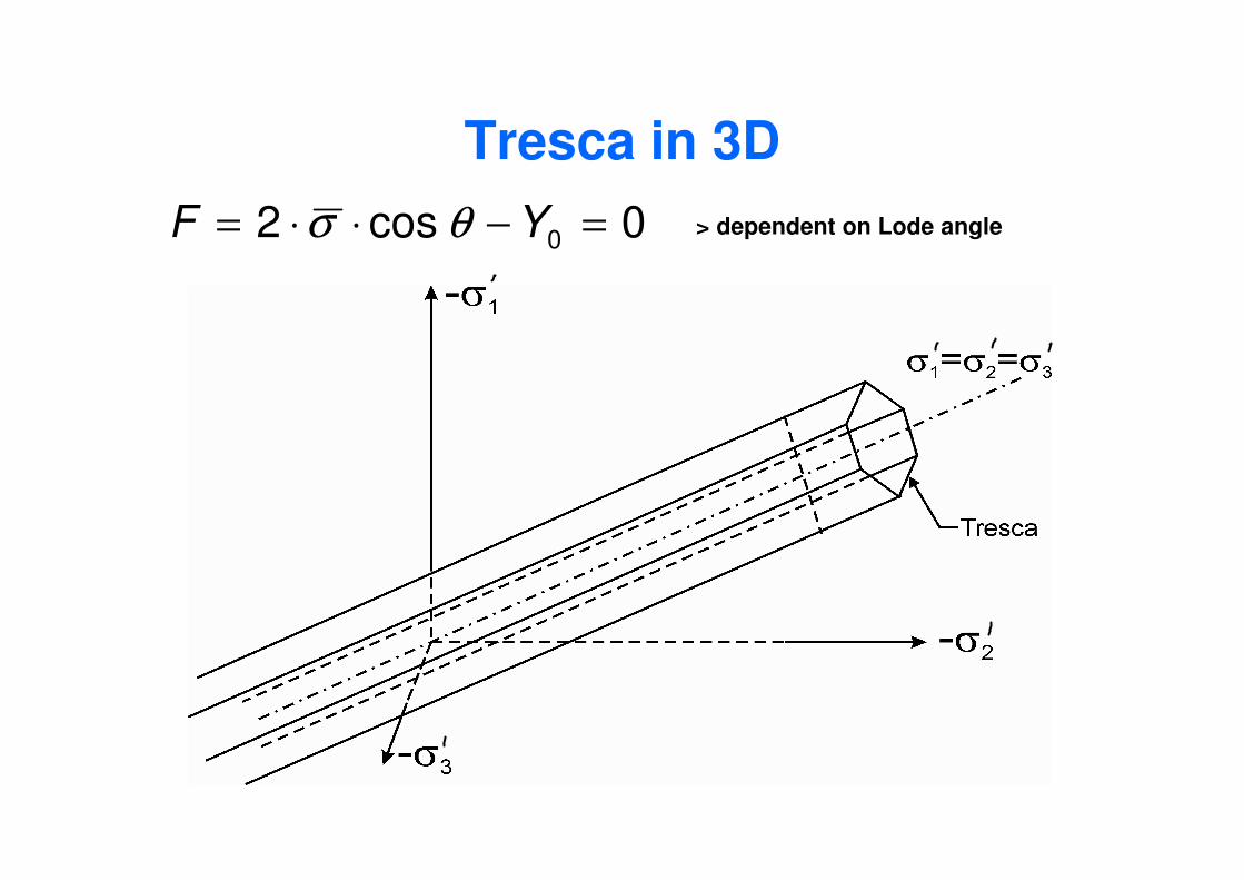
Tresca in 3D
0cos2 0 =−⋅⋅= YF θσ > dependent on Lode angle
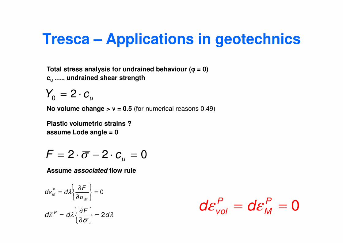
Tresca – Applications in geotechnics
ucY ⋅= 20
Total stress analysis for undrained behaviour (ϕϕϕϕ = 0)
cu ….. undrained shear strength
No volume change > νννν = 0.5 (for numerical reasons 0.49)
Plastic volumetric strains ?
022 =⋅−⋅= ucF σ
0=
∂
∂=
M
PM
Fdd
σλε
λσ
λε dF
dd P 2=
∂
∂=
0== PM
Pvol dd εε
Plastic volumetric strains ?
assume Lode angle = 0
Assume associated flow rule
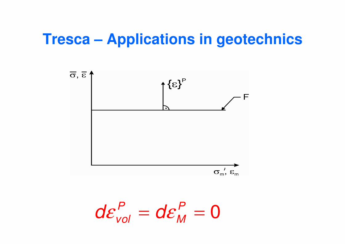
Tresca – Applications in geotechnics
0== PM
Pvol dd εε
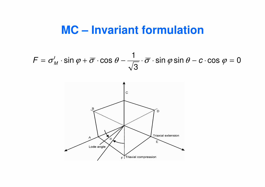
MC – Invariant formulation
0cossinsin3
1cossin =⋅−⋅⋅−⋅+⋅= ϕθϕσθσϕσ cF M
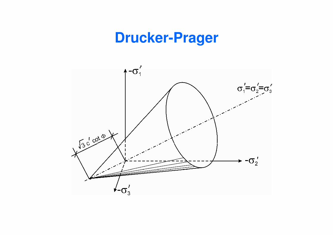
Drucker-Prager

Drucker-Prager vs MC
Drucker-Prager and Mohr-Coulomb criteria in ππππ - plane
Nonlinear FE and solution techniquestechniques
(as in PLAXIS)
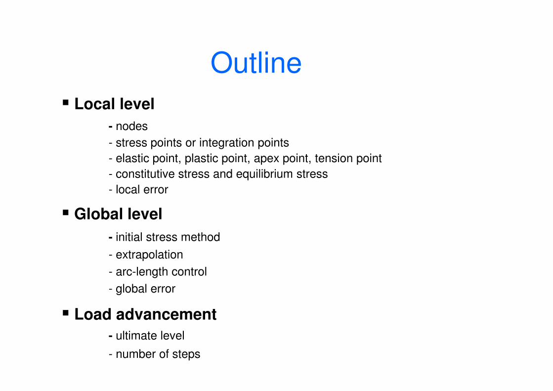
� Local level
- nodes
- stress points or integration points
- elastic point, plastic point, apex point, tension point
- constitutive stress and equilibrium stress
- local error
Outline
- local error
� Global level
- initial stress method
- extrapolation
- arc-length control
- global error
� Load advancement
- ultimate level
- number of steps
Main Topics on Non-linear Analysis
• Calculation
• Basic Concepts and Algorithms
• Local Level
• Global Level
• Load Advancement
Calculation
Initial situation
• Geometry (mesh, loads, boundary conditions)
• Material models and parameters• Material models and parameters
• Initial stresses and pore pressures
• Initial values of state variables
Calculation
Calculation phases
• Calculation types
– Plastic– Plastic
– Consolidation
– Phi-c reduction (limit state analysis)
Calculation (continues)
Calculation phases (continues)
• Loading input
– Staged construction
• Switch on/off parts of geometry• Switch on/off parts of geometry
• Switch on/off structural elements (beams, anchors)
• Switch on/off loads (change input values)
• Change pore pressures
– Total Multipliers (L.A. Ultimate level)
– Incremental Multipliers (L.A. Number of steps)
Calculation (continues)
Output
• Displacements, stresses, forces etc. per step/phase
– Displacements and pore pressures are nodal – Displacements and pore pressures are nodal values
– Stresses, strains and state variables are Gauss point level values
• Load-displacement curves
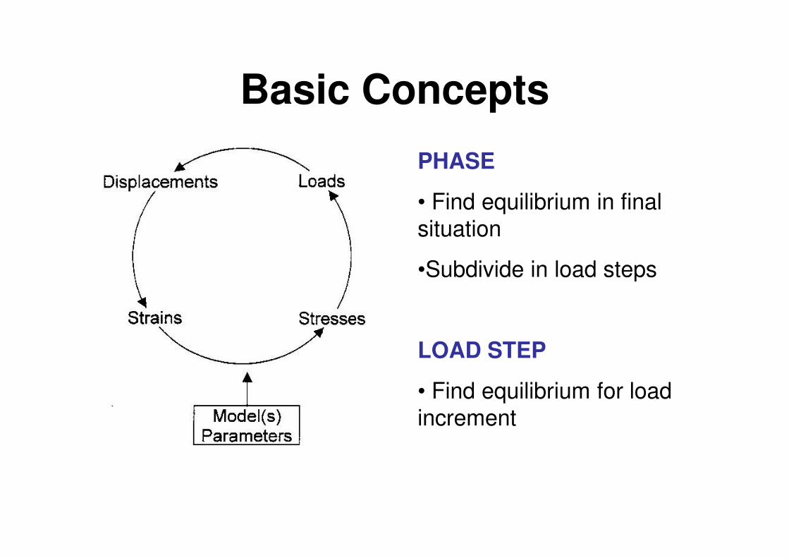
PHASE
• Find equilibrium in final situation
•Subdivide in load steps
Basic Concepts
•Subdivide in load steps
LOAD STEP
• Find equilibrium for load increment
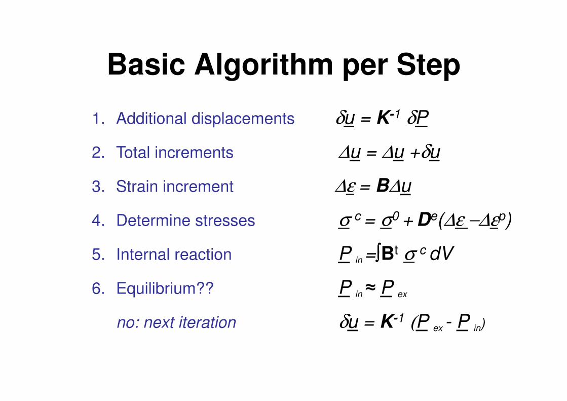
Basic Algorithm per Step
1. Additional displacements δu = K-1 δP
2. Total increments ∆u = ∆u +δu
3. Strain increment ∆ε = B∆u
4. Determine stresses σ c = σ0 + De(∆ε −∆εp)
5. Internal reaction P in =∫∫∫∫Bt σ c dV
6. Equilibrium?? P in ≈ P ex
no: next iteration δu = K-1 (P ex - P in)
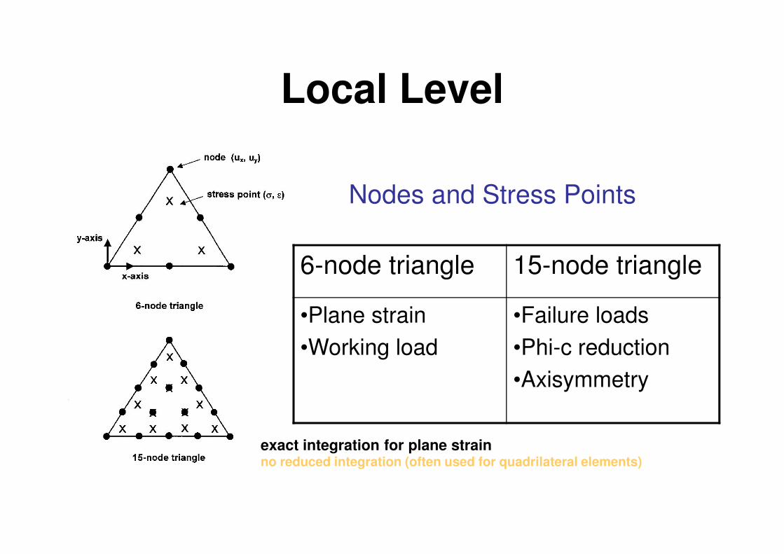
Local Level
6-node triangle 15-node triangle
Nodes and Stress Points
6-node triangle 15-node triangle
•Plane strain
•Working load
•Failure loads
•Phi-c reduction
•Axisymmetry
exact integration for plane strainno reduced integration (often used for quadrilateral elements)
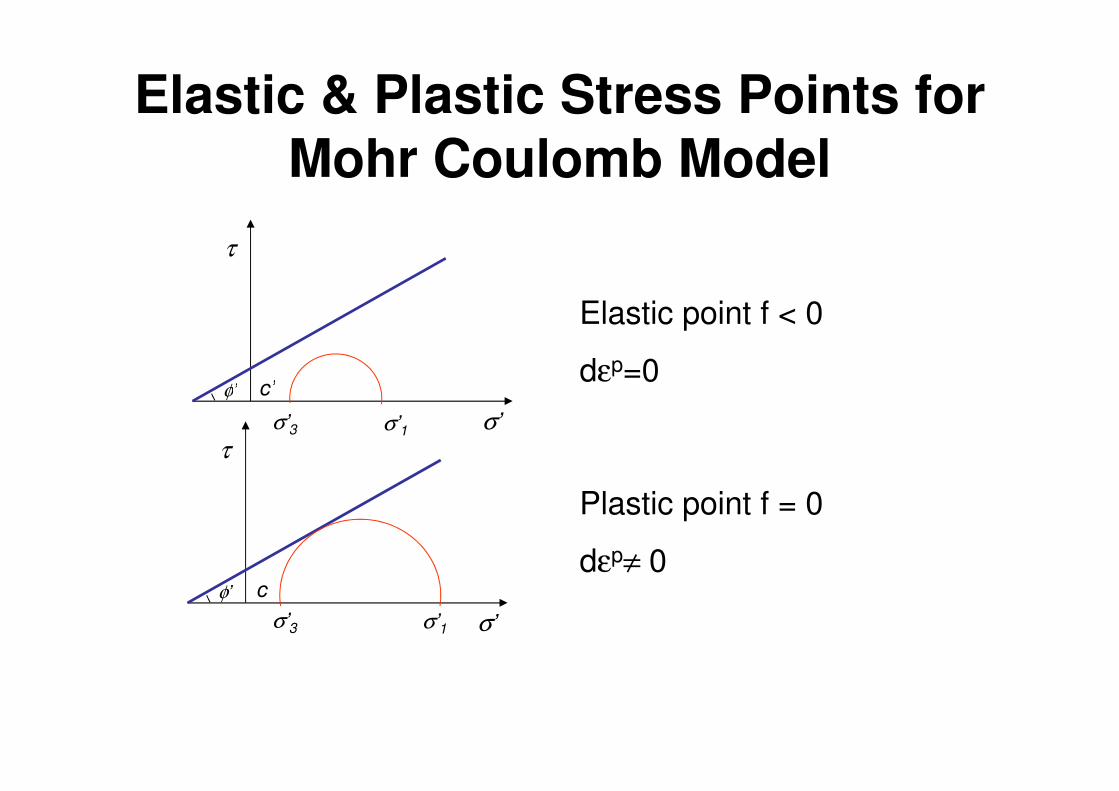
Elastic & Plastic Stress Points for Mohr Coulomb Model
τ
c’φ’
Elastic point f < 0
dεp=0
τ
σ’
cφ’
σ’
c’φ’
σ1σ3
σ’3 σ’1
Plastic point f = 0
dεp≠ 0
σ’3 σ’1
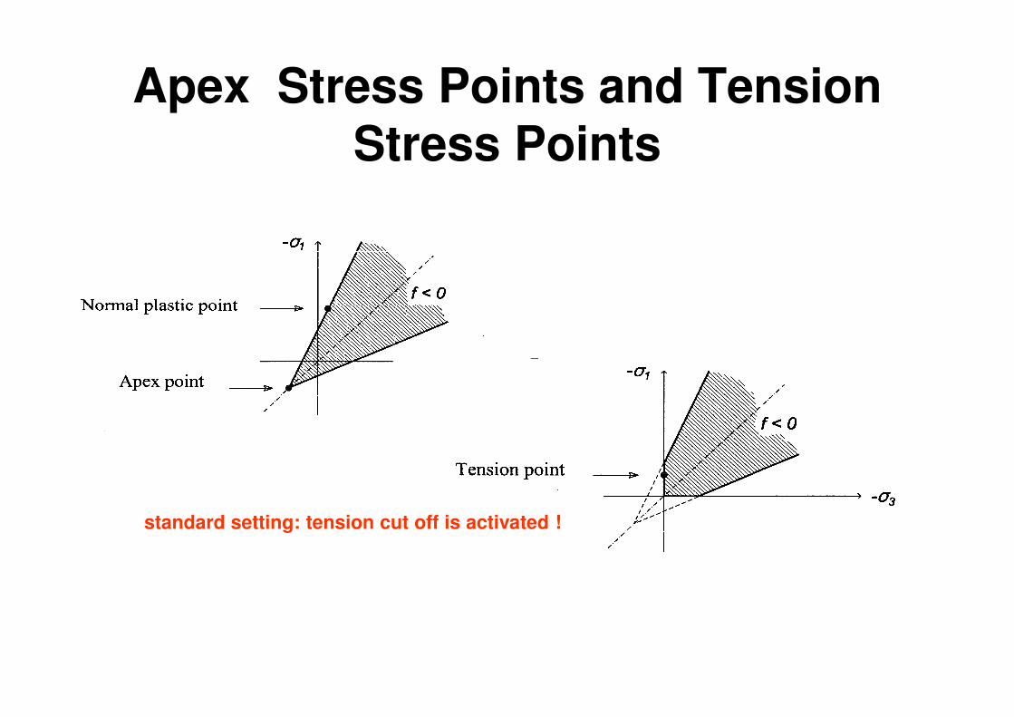
Apex Stress Points and Tension Stress Points
standard setting: tension cut off is activated !
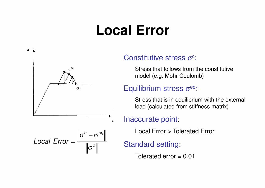
Local Error
Constitutive stress σc:
Stress that follows from the constitutive model (e.g. Mohr Coulomb)
Equilibrium stress σeq:
Stress that is in equilibrium with the external load (calculated from stiffness matrix)
Inaccurate point:
Local Error > Tolerated Error
Standard setting:
Tolerated error = 0.01
c
eqc
ErrorLocalσ
σ−σ=
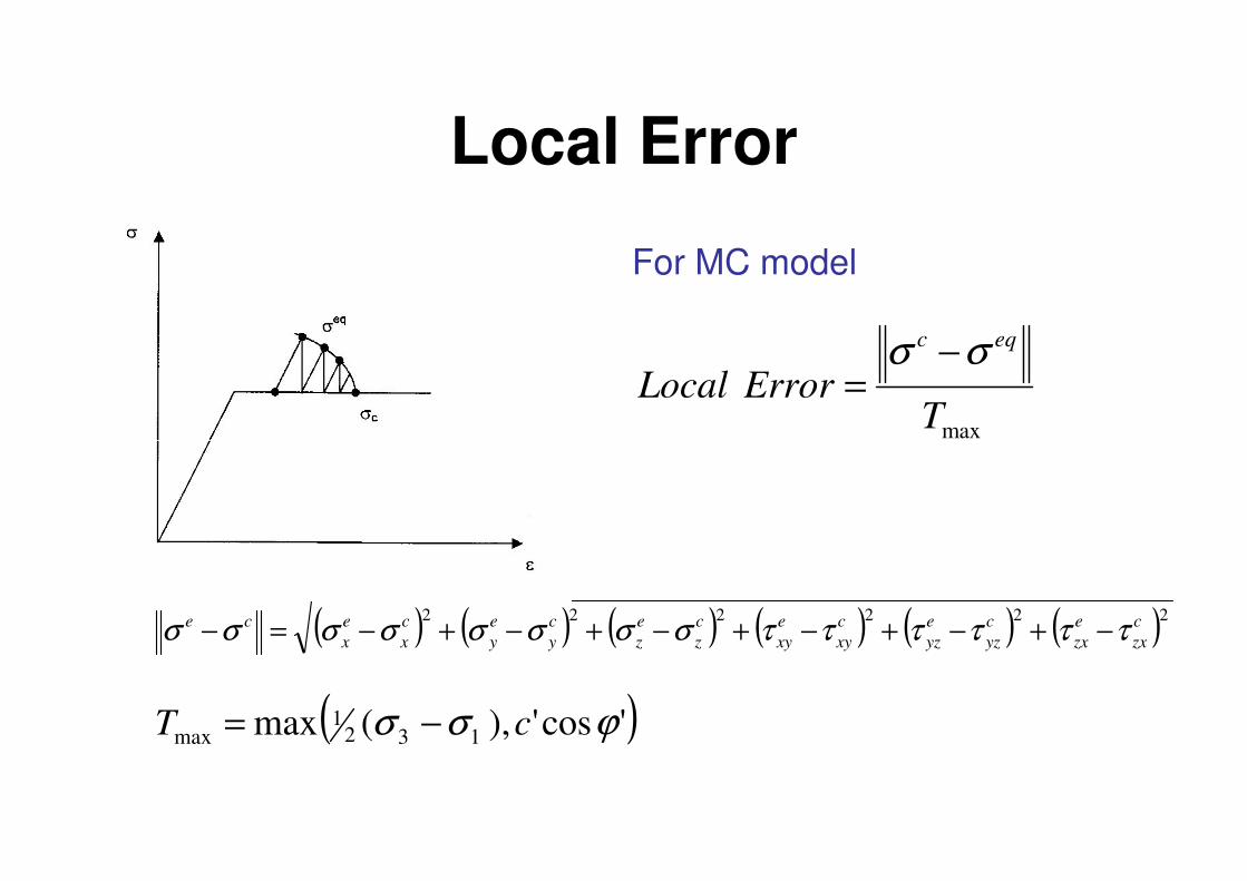
Local Error
For MC model
maxTErrorLocal
eqc σσ −=
( ) ( ) ( ) ( ) ( ) ( )222222 c
zx
e
zx
c
yz
e
yz
c
xy
e
xy
c
z
e
z
c
y
e
y
c
x
e
x
ce ττττττσσσσσσσσ −+−+−+−+−+−=−
max
( )'cos'),(max 1321
max ϕσσ cT −=
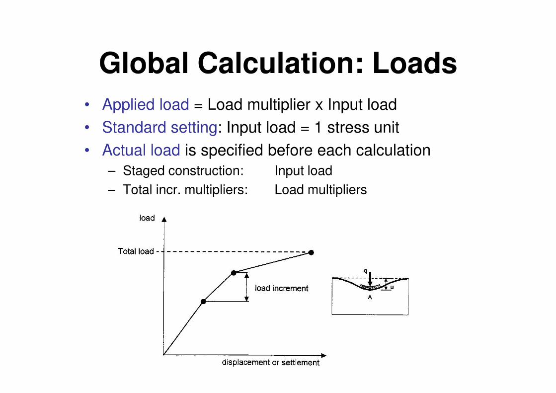
Global Calculation: Loads
• Applied load = Load multiplier x Input load
• Standard setting: Input load = 1 stress unit
• Actual load is specified before each calculation
– Staged construction: Input load
– Total incr. multipliers: Load multipliers– Total incr. multipliers: Load multipliers
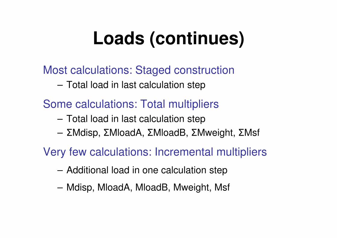
Loads (continues)
Most calculations: Staged construction
– Total load in last calculation step
Some calculations: Total multipliers
– Total load in last calculation step– Total load in last calculation step
– ΣMdisp, ΣMloadA, ΣMloadB, ΣMweight, ΣMsf
Very few calculations: Incremental multipliers
– Additional load in one calculation step
– Mdisp, MloadA, MloadB, Mweight, Msf
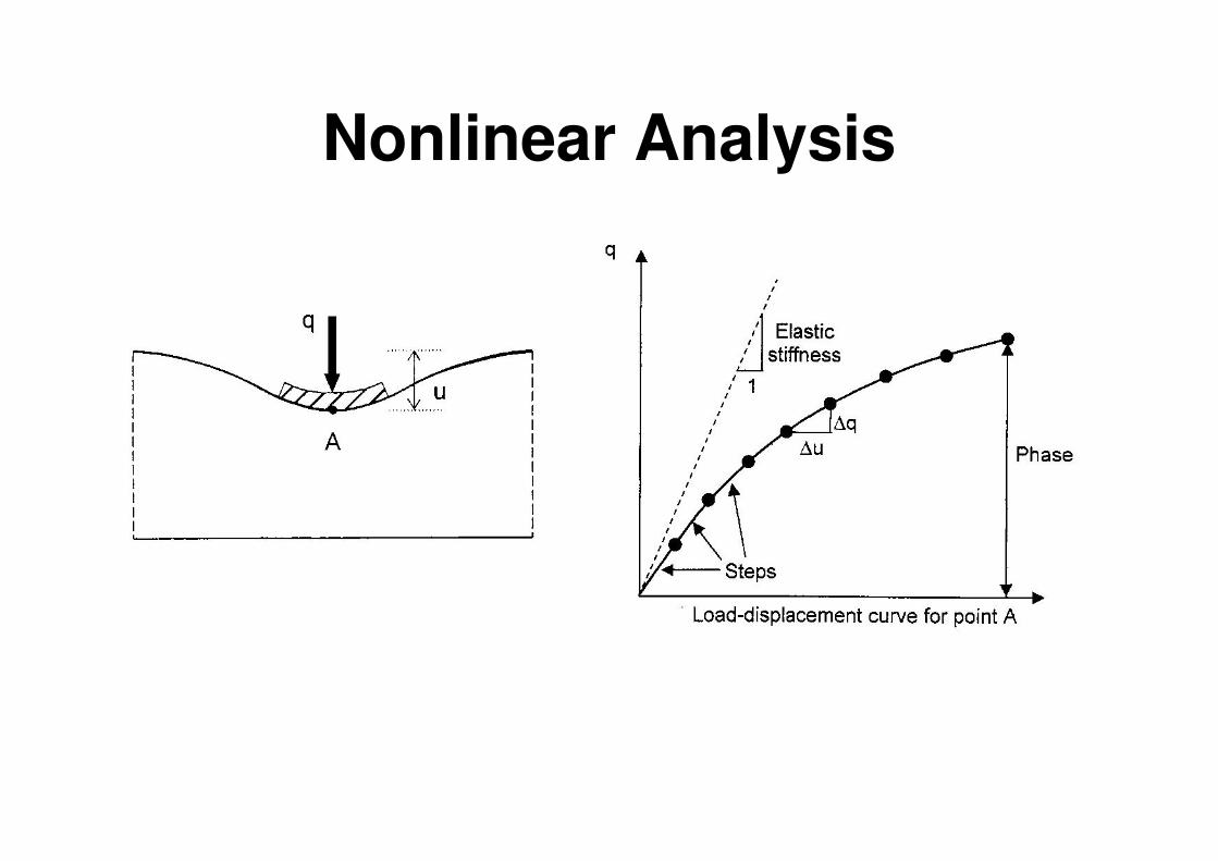
Nonlinear Analysis
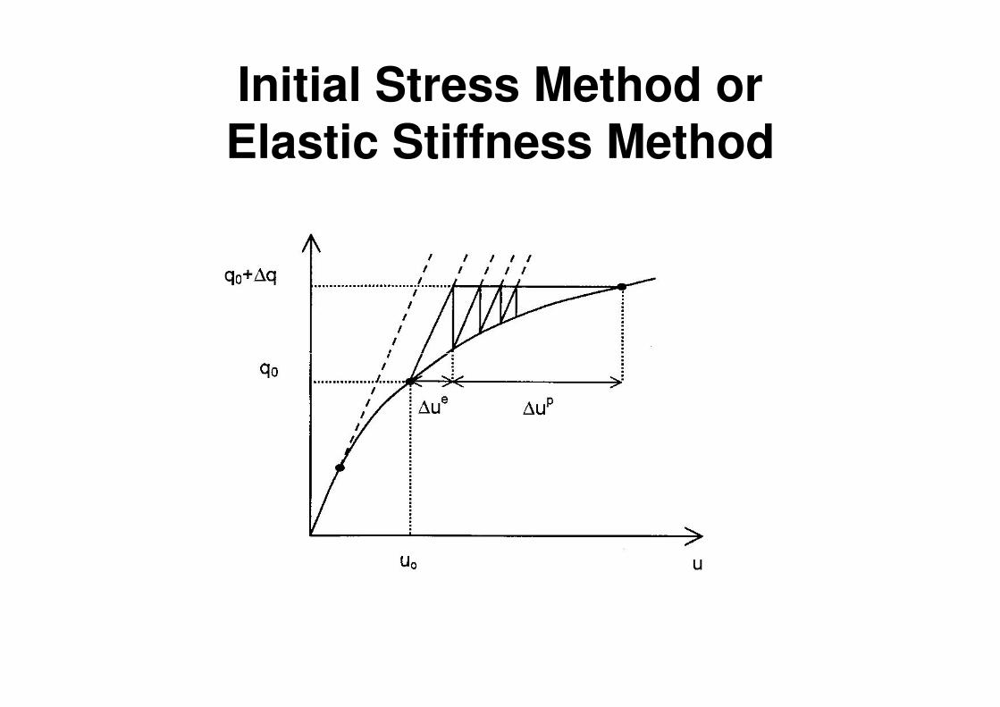
Initial Stress Method orElastic Stiffness Method
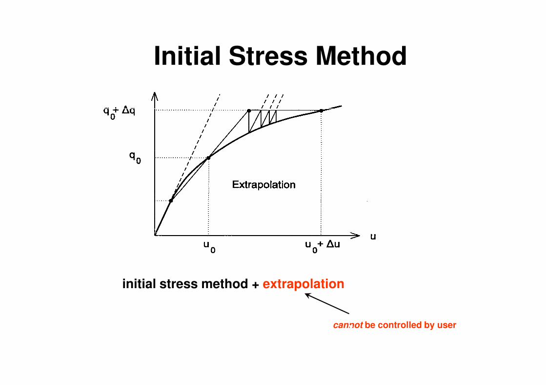
Initial Stress Method
initial stress method + extrapolation
cannot be controlled by user
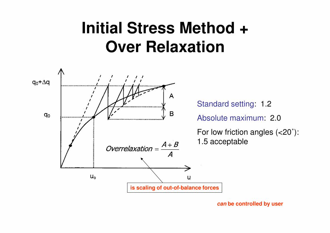
Initial Stress Method +Over Relaxation
Standard setting: 1.2
Absolute maximum: 2.0Absolute maximum: 2.0
For low friction angles (<20˚): 1.5 acceptable
is scaling of out-of-balance forces
can be controlled by user
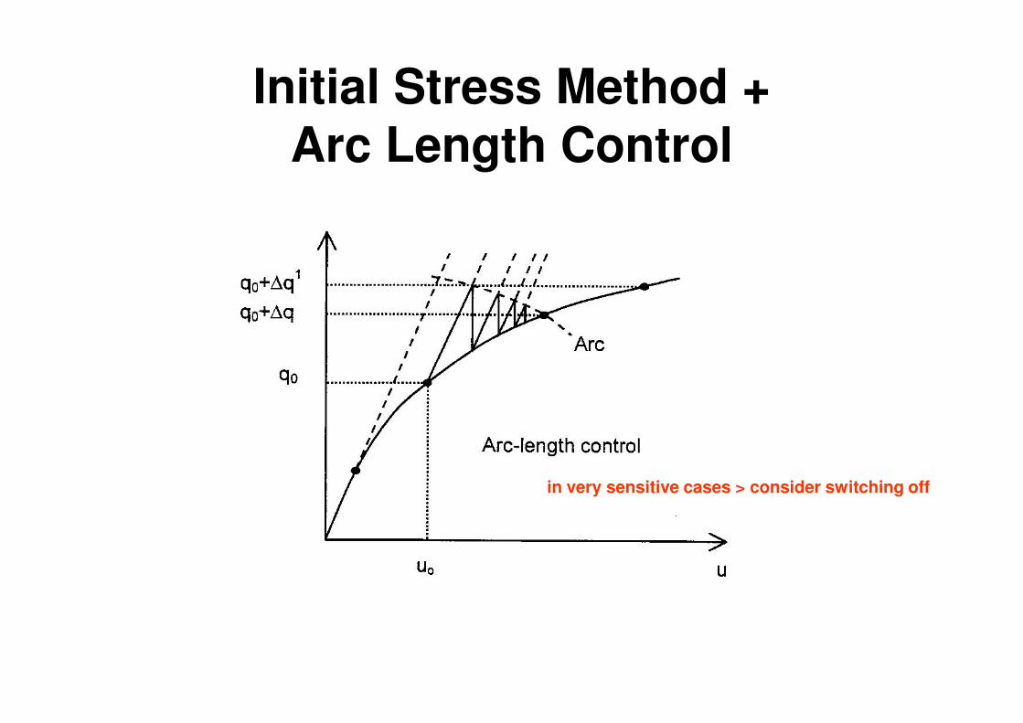
Initial Stress Method +Arc Length Control
in very sensitive cases > consider switching off
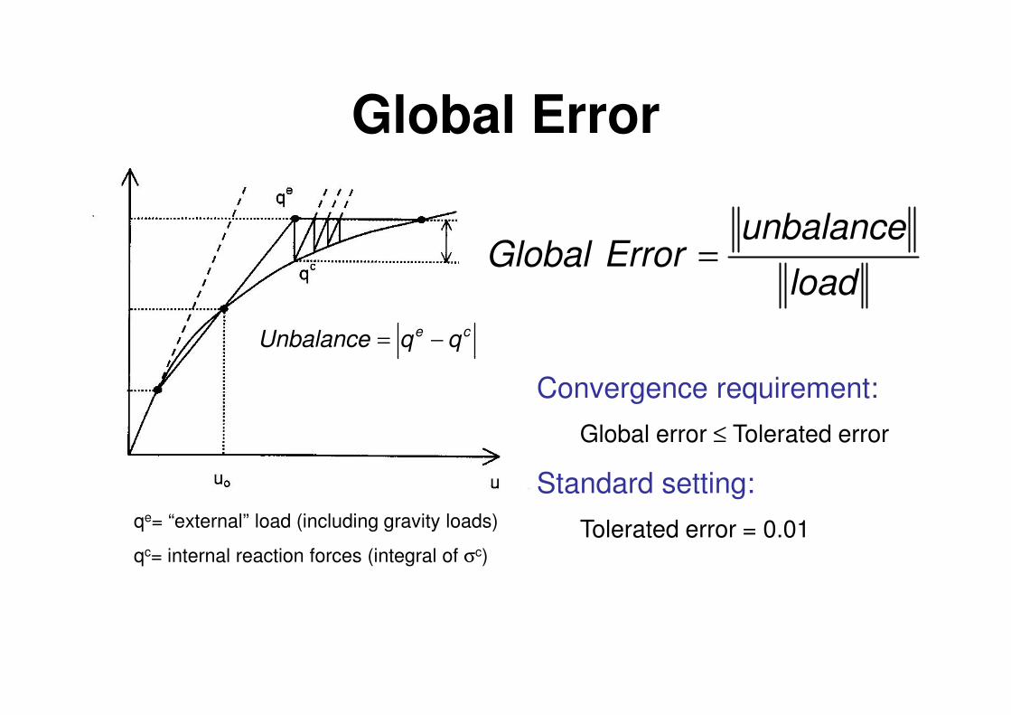
Global Error
load
unbalanceErrorGlobal =
ce qqUnbalance −=
qe= “external” load (including gravity loads)
qc= internal reaction forces (integral of σc)
Convergence requirement:
Global error ≤ Tolerated error
Standard setting:
Tolerated error = 0.01
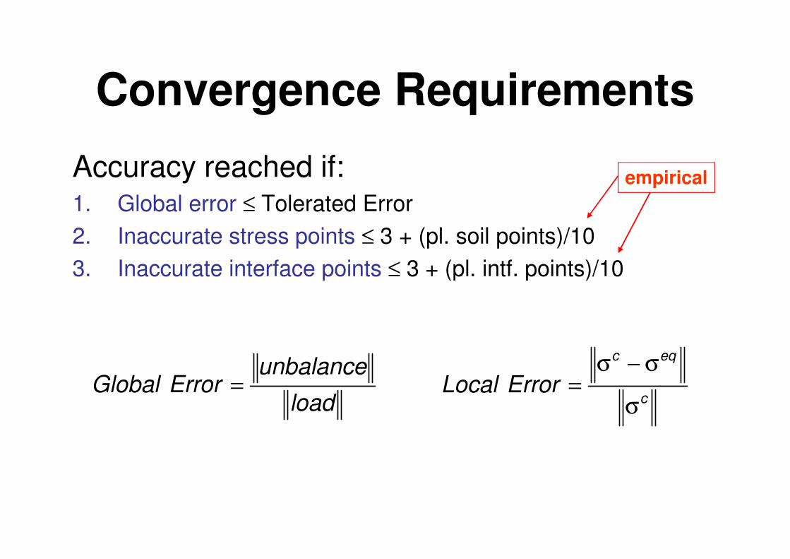
Convergence Requirements
Accuracy reached if:1. Global error ≤ Tolerated Error
2. Inaccurate stress points ≤ 3 + (pl. soil points)/10
3. Inaccurate interface points ≤ 3 + (pl. intf. points)/10
empirical
3. Inaccurate interface points ≤ 3 + (pl. intf. points)/10
c
eqc
ErrorLocalσ
σ−σ=
load
unbalanceErrorGlobal =
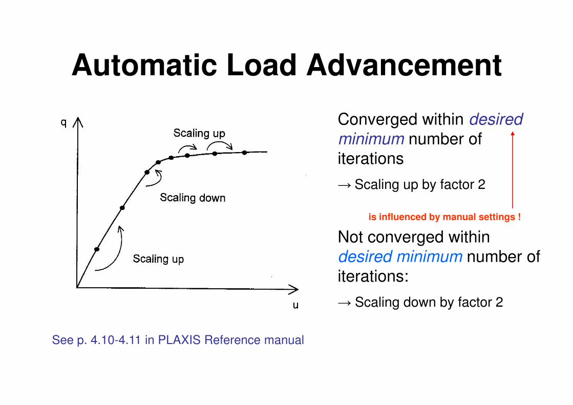
Automatic Load Advancement
Converged within desired
minimum number of iterations
→ Scaling up by factor 2
Not converged within desired minimum number of iterations:
→ Scaling down by factor 2
is influenced by manual settings !
See p. 4.10-4.11 in PLAXIS Reference manual
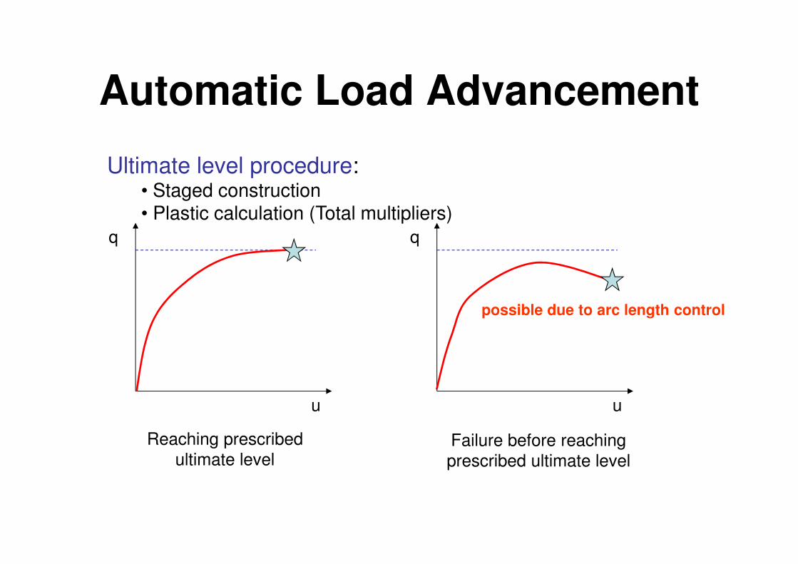
Automatic Load Advancement
Ultimate level procedure:• Staged construction• Plastic calculation (Total multipliers)
uu
Reaching prescribed ultimate level
Failure before reaching prescribed ultimate level
possible due to arc length control
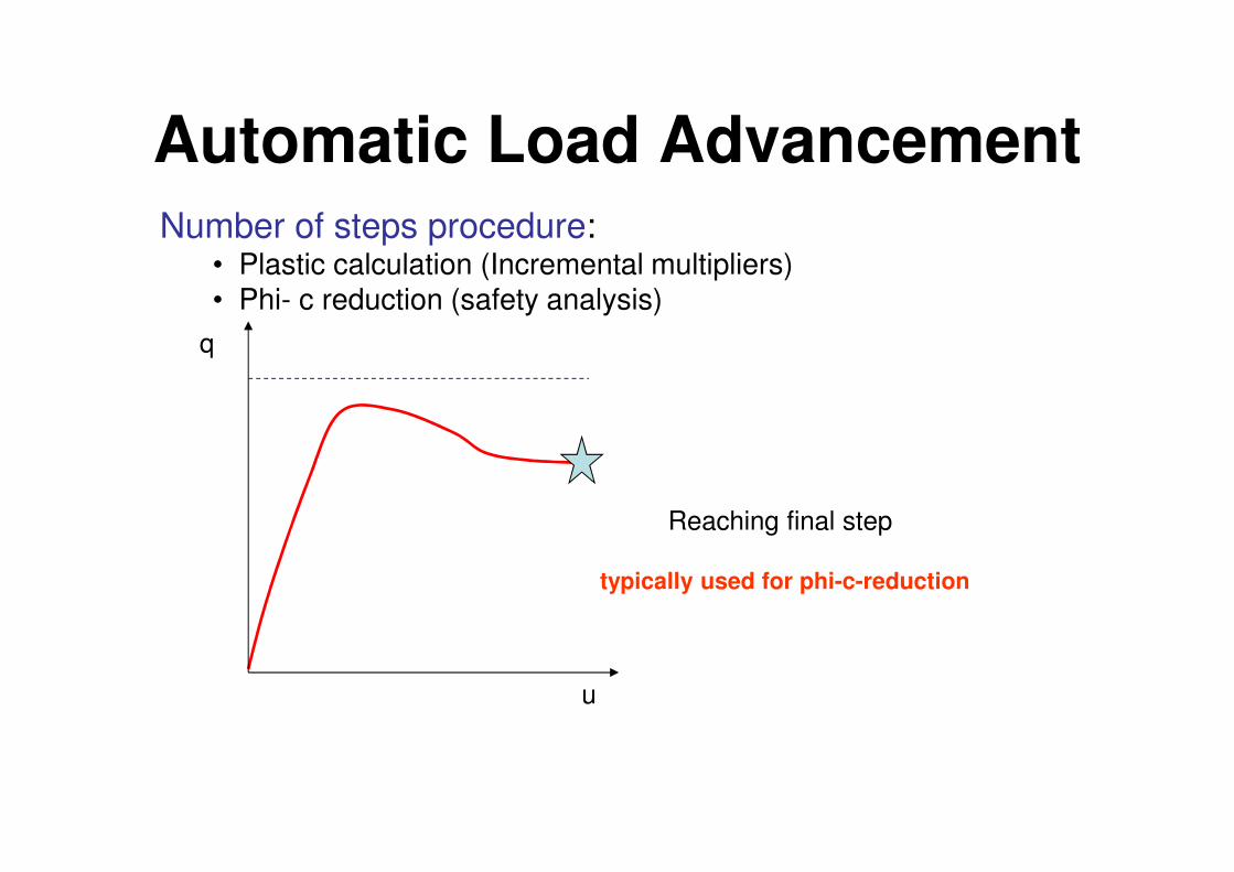
Automatic Load AdvancementNumber of steps procedure:
• Plastic calculation (Incremental multipliers)• Phi- c reduction (safety analysis)
q
u
Reaching final step
typically used for phi-c-reduction
![a] [Ptuprints.ulb.tu-darmstadt.de/420/3/habil_elektr_3.pdf · gle crystal plasticity, multi{surface plasticity, textur development 6.1 Introduction The treatment of single crystal](https://static.fdocument.org/doc/165x107/5f0f53897e708231d4439b67/a-gle-crystal-plasticity-multisurface-plasticity-textur-development-61-introduction.jpg)


![Title: Plasticity Effects in Incremental Slitting Measurement of · PDF filethicknesses greater 160 mm [6]. Slitting has measured stresses of very low magnitude quite precisely [7-10].](https://static.fdocument.org/doc/165x107/5a9fd36a7f8b9a0d158d57fd/title-plasticity-effects-in-incremental-slitting-measurement-of-greater-160-mm.jpg)