
Radial Basis Function Methods - Applied...
27
Oliver Smithies Lecture December 1, 2010 Sponsored by benefaction from Prof. Oliver Smithies to Balliol College Radial Basis Function Methods: Developments and Applications to Planetary Scale Flows Bengt Fornberg University of Colorado Boulder, Department of Applied Mathematics in collaboration with Natasha Flyer NCAR, IMAGe Institute for Mathematics Applied to the Geosciences Slide 1 of 27
Transcript of Radial Basis Function Methods - Applied...
Oliver Smithies Lecture December 1, 2010Sponsored by benefaction from Prof. Oliver Smithies to Balliol College
Radial Basis Function Methods:
Developments and Applications toPlanetary Scale Flows
Bengt Fornberg University of Colorado Boulder,
Department of Applied Mathematics
in collaboration with
Natasha Flyer NCAR, IMAGe
Institute for Mathematics Applied to the Geosciences
Slide 1 of 27
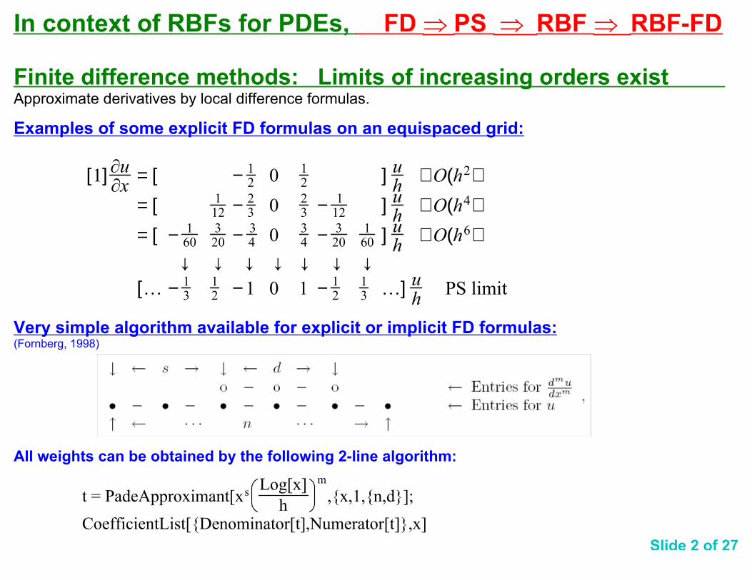
In context of RBFs for PDEs, FD ⇒ PS ⇒ RBF ⇒ RBF-FD
Finite difference methods: Limits of increasing orders exist Approximate derivatives by local difference formulas.
Examples of some explicit FD formulas on an equispaced grid:
[1]ØuØx
= [ − 12 0
12 ] u
h+O(h2)
= [ 112 − 2
3 023 − 1
12 ] uh
+O(h4)= [ − 1
60320 − 3
4 034 − 3
20160 ] u
h+O(h6)
o o o o o o o
[¢ − 13
12 − 1 0 1 − 1
213 ¢] u
hPS limit
Very simple algorithm available for explicit or implicit FD formulas:(Fornberg, 1998)
All weights can be obtained by the following 2-line algorithm:
t = PadeApproximant[xsLog[x]
h
m
,{x,1,{n,d}];
CoefficientList[{Denominator[t],Numerator[t]},x]
Slide 2 of 27
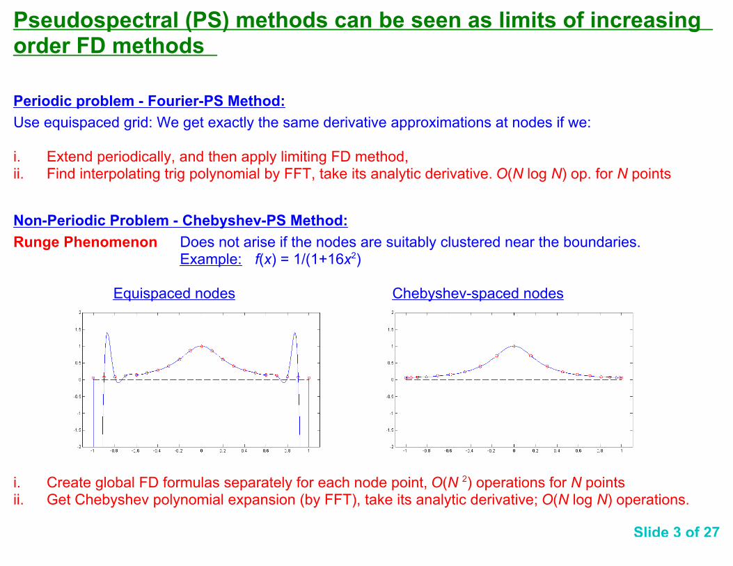
Pseudospectral (PS) methods can be seen as limits of increasing order FD methods
Periodic problem - Fourier-PS Method:
Use equispaced grid: We get exactly the same derivative approximations at nodes if we:
i. Extend periodically, and then apply limiting FD method,ii. Find interpolating trig polynomial by FFT, take its analytic derivative. O(N log N) op. for N points
Non-Periodic Problem - Chebyshev-PS Method:
Runge Phenomenon Does not arise if the nodes are suitably clustered near the boundaries.Example: f(x) = 1/(1+16x2)
Equispaced nodes Chebyshev-spaced nodes
i. Create global FD formulas separately for each node point, O(N 2) operations for N pointsii. Get Chebyshev polynomial expansion (by FFT), take its analytic derivative; O(N log N) operations.
Slide 3 of 27
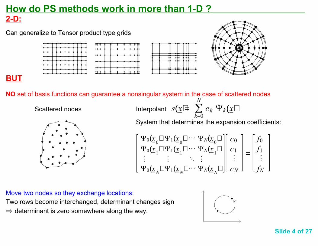
How do PS methods work in more than 1-D ? 2-D:
Can generalize to Tensor product type grids
BUT
NO set of basis functions can guarantee a nonsingular system in the case of scattered nodes
Scattered nodes Interpolant s(x) = �k=0
N
ck �k(x)System that determines the expansion coefficients:
�0(x0) �1(x
0) £ �N(x
0)
�0(x1) �1(x
1) £ �N(x
1)
§ § • §
�0(xN
) �1(xN
) £ �N(xN)
c0
c1
§
cN
=
f0f1§
fN
Move two nodes so they exchange locations:
Two rows become interchanged, determinant changes sign
fl determinant is zero somewhere along the way.
Slide 4 of 27
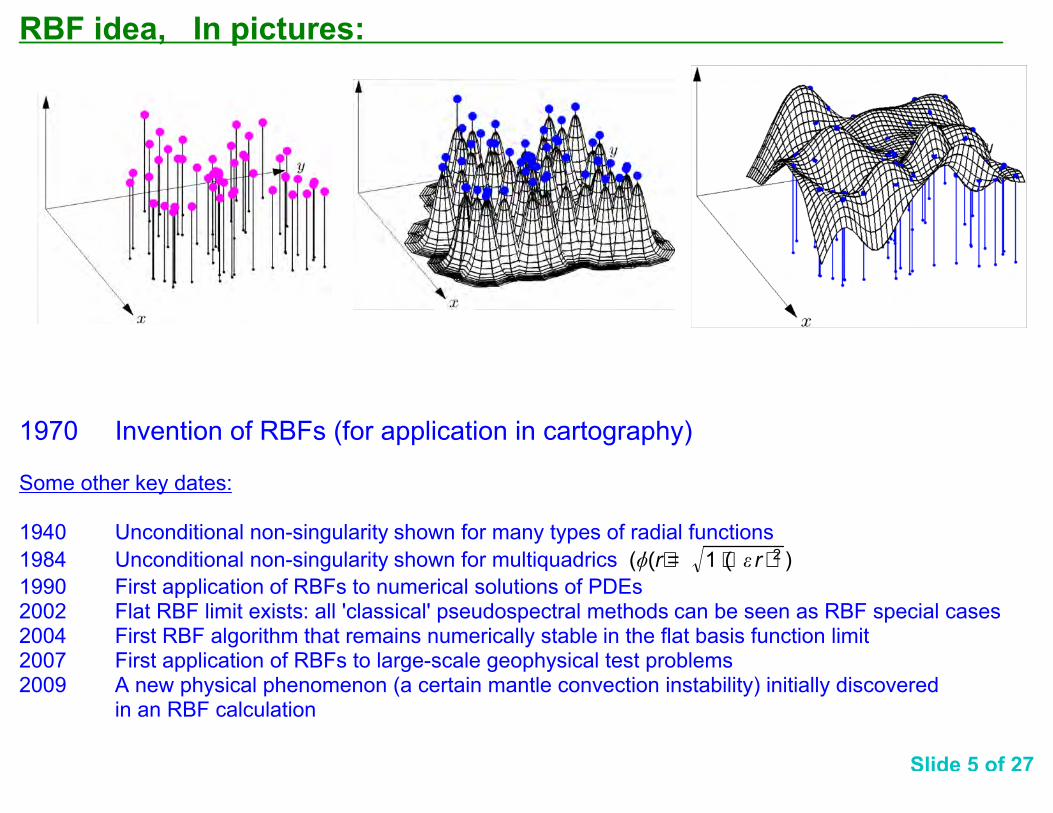
RBF idea, In pictures:
1970 Invention of RBFs (for application in cartography)
Some other key dates:
1940 Unconditional non-singularity shown for many types of radial functions
1984 Unconditional non-singularity shown for multiquadrics ( )�(r) = 1 + (� r )21990 First application of RBFs to numerical solutions of PDEs2002 Flat RBF limit exists: all 'classical' pseudospectral methods can be seen as RBF special cases 2004 First RBF algorithm that remains numerically stable in the flat basis function limit2007 First application of RBFs to large-scale geophysical test problems2009 A new physical phenomenon (a certain mantle convection instability) initially discovered
in an RBF calculation
Slide 5 of 27
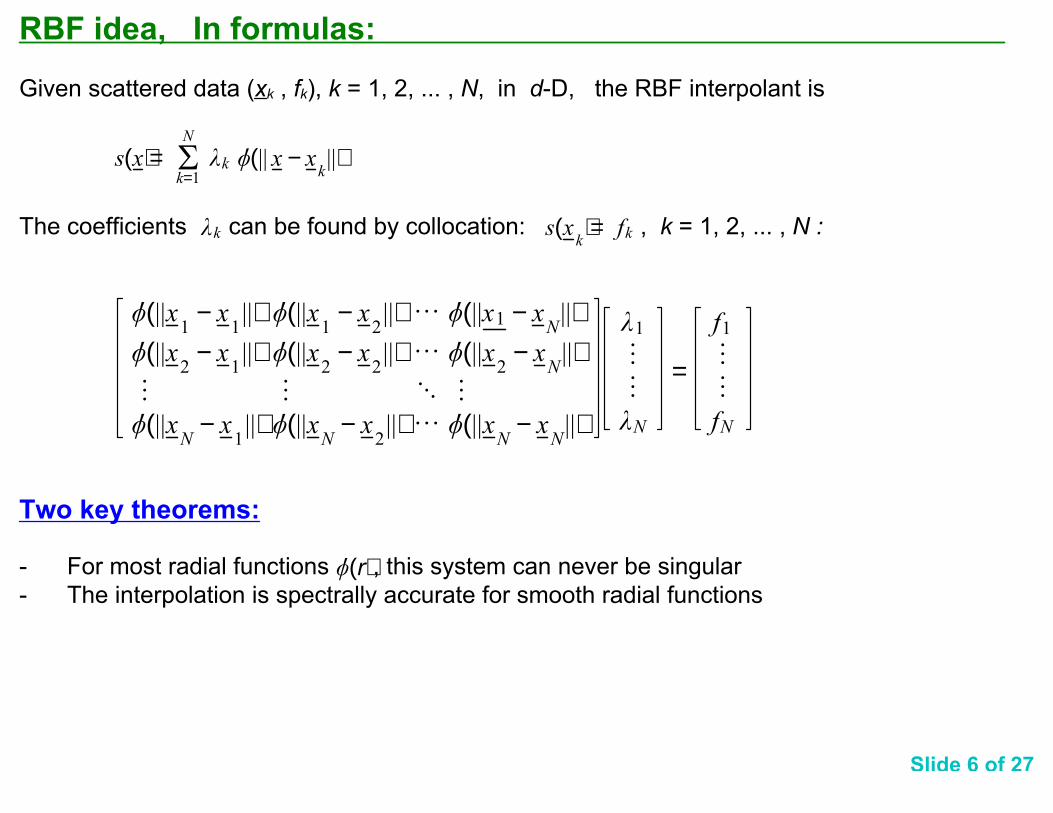
RBF idea, In formulas:
Given scattered data (xk , fk), k = 1, 2, ... , N, in d-D, the RBF interpolant is
s(x) = �k=1
N
�k �(|| x − xk||)
The coefficients can be found by collocation: , k = 1, 2, ... , N :�k s(xk) = fk
�(||x1
− x1||) �(||x
1− x
2||) £ �(||x1 − x
N||)
�(||x2
− x1||) �(||x
2− x
2||) £ �(||x
2− x
N||)
§ § •§
�(||xN
− x1||) �(||x
N− x
2||)£ �(||x
N− x
N||)
�1
§
§
�N
=
f1§
§
fN
Two key theorems:
- For most radial functions , this system can never be singular�(r)- The interpolation is spectrally accurate for smooth radial functions
Slide 6 of 27
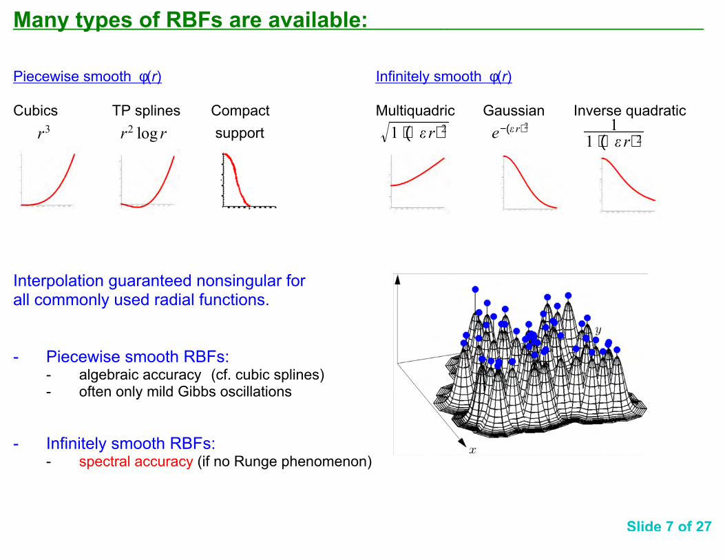
Many types of RBFs are available:
Piecewise smooth φ(r) Infinitely smooth φ(r)
Cubics TP splines Compact Multiquadric Gaussian Inverse quadratic
support r3 r2 log r 1 + (� r)2 e−(� r)2 11 + (� r)2
Interpolation guaranteed nonsingular forall commonly used radial functions.
- Piecewise smooth RBFs:- algebraic accuracy (cf. cubic splines)- often only mild Gibbs oscillations
- Infinitely smooth RBFs:- spectral accuracy (if no Runge phenomenon)
Slide 7 of 27
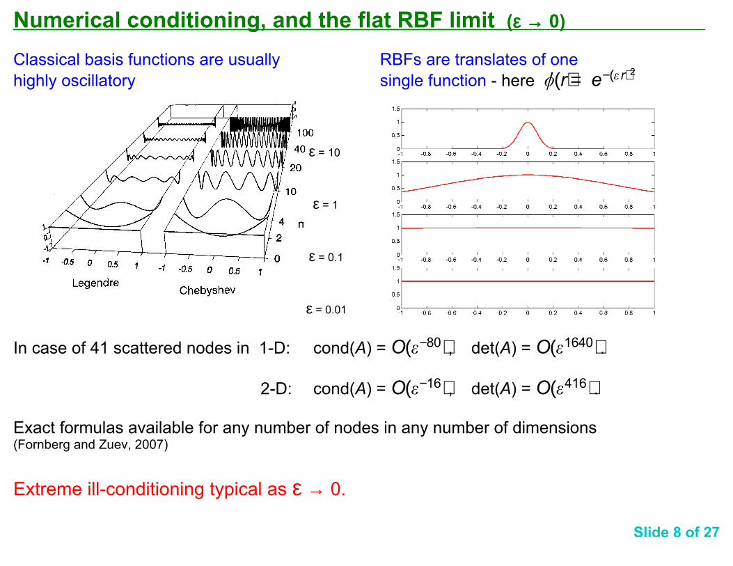
Numerical conditioning, and the flat RBF limit (ε →ε →ε →ε → 0)
Classical basis functions are usually RBFs are translates of one
highly oscillatory single function - here �(r) = e−(� r)2
ε = 10
ε = 1
ε = 0.1
ε = 0.01
In case of 41 scattered nodes in 1-D: cond(A) = , det(A) = .O(�−80) O(�1640)
2-D: cond(A) = , det(A) = .O(�−16) O(�416)
Exact formulas available for any number of nodes in any number of dimensions(Fornberg and Zuev, 2007)
Extreme ill-conditioning typical as ε → 0.
Slide 8 of 27
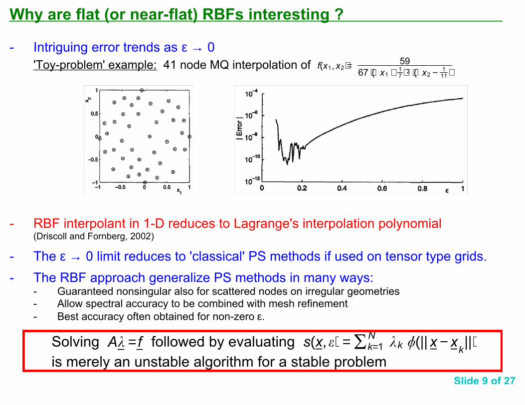
Why are flat (or near-flat) RBFs interesting ?
- Intriguing error trends as ε → 0'Toy-problem' example: 41 node MQ interpolation of f(x1,x2) = 59
67 + (x1 + 17 )2 + (x2 − 1
11 )
- RBF interpolant in 1-D reduces to Lagrange's interpolation polynomial (Driscoll and Fornberg, 2002)
- The ε → 0 limit reduces to 'classical' PS methods if used on tensor type grids.- The RBF approach generalize PS methods in many ways:
- Guaranteed nonsingular also for scattered nodes on irregular geometries- Allow spectral accuracy to be combined with mesh refinement
- Best accuracy often obtained for non-zero ε.
Solving followed by evaluating A� = f s(x, �) =�k=1N�k �(||x − x
k||)
is merely an unstable algorithm for a stable problem
Slide 9 of 27
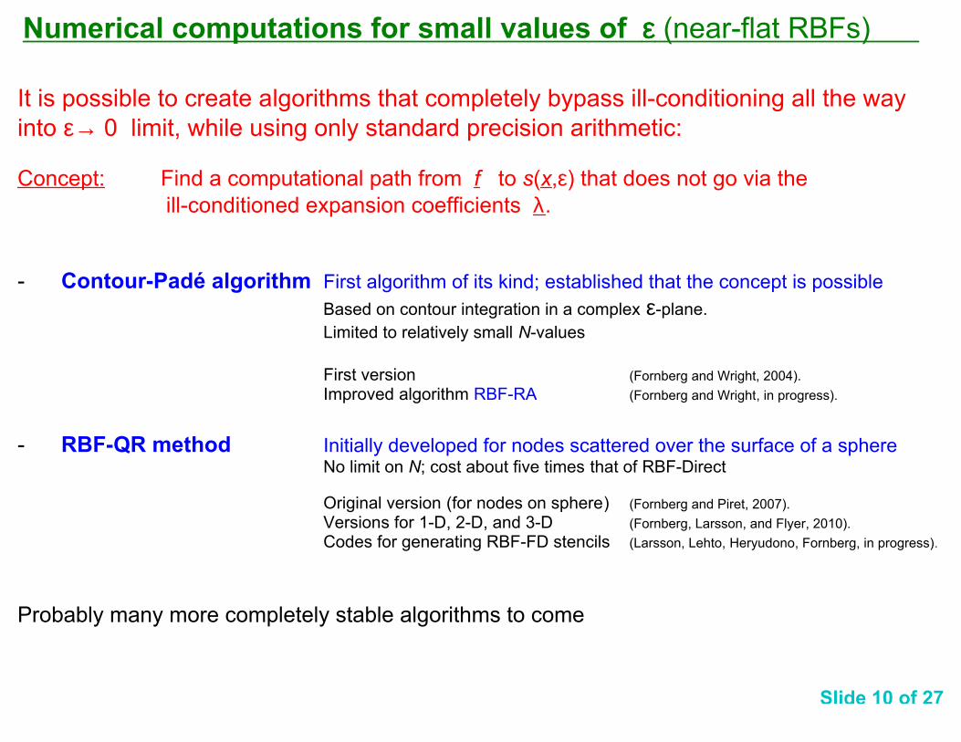
Numerical computations for small values of εεεε (near-flat RBFs)
It is possible to create algorithms that completely bypass ill-conditioning all the way
into ε→ 0 limit, while using only standard precision arithmetic:
Concept: Find a computational path from f to s(x,ε) that does not go via theill-conditioned expansion coefficients λ.
- Contour-Padé algorithm First algorithm of its kind; established that the concept is possible
Based on contour integration in a complex ε-plane. Limited to relatively small N-values
First version (Fornberg and Wright, 2004).
Improved algorithm RBF-RA (Fornberg and Wright, in progress).
- RBF-QR method Initially developed for nodes scattered over the surface of a sphereNo limit on N; cost about five times that of RBF-Direct
Original version (for nodes on sphere) (Fornberg and Piret, 2007).
Versions for 1-D, 2-D, and 3-D (Fornberg, Larsson, and Flyer, 2010).
Codes for generating RBF-FD stencils (Larsson, Lehto, Heryudono, Fornberg, in progress).
Probably many more completely stable algorithms to come
Slide 10 of 27
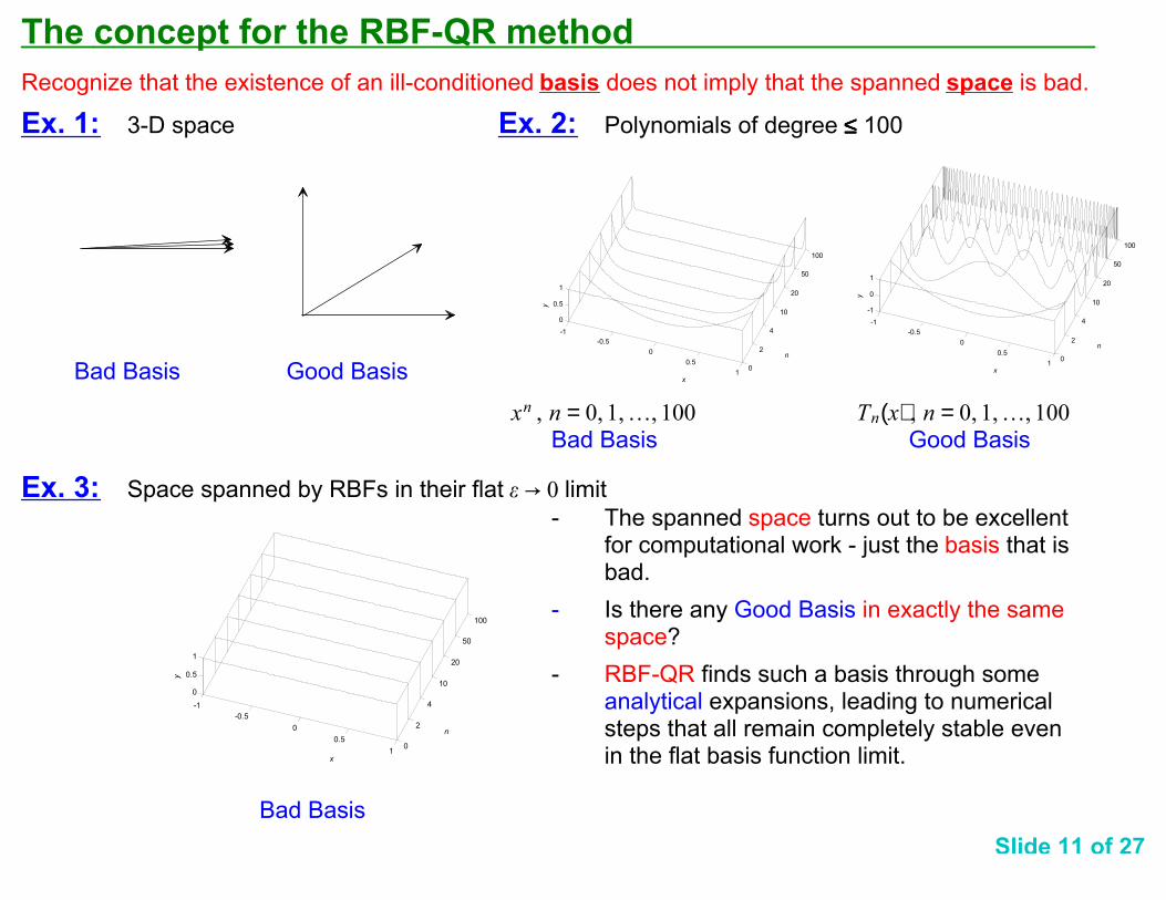
The concept for the RBF-QR method
Recognize that the existence of an ill-conditioned basis does not imply that the spanned space is bad.
Ex. 1: 3-D space Ex. 2: Polynomials of degree ≤≤≤≤ 100
Bad Basis Good Basis
xn , n = 0, 1,¢, 100 Tn(x) , n = 0, 1,¢, 100
Bad Basis Good Basis
Ex. 3: Space spanned by RBFs in their flat limit� d 0
- The spanned space turns out to be excellentfor computational work - just the basis that isbad.
- Is there any Good Basis in exactly the same space?
- RBF-QR finds such a basis through someanalytical expansions, leading to numerical steps that all remain completely stable evenin the flat basis function limit.
Bad Basis
Slide 11 of 27
-1
-0.5
0
0.5
10
2
4
10
20
50
100
-1
0
1
n
x
y
-1
-0.5
0
0.5
10
2
4
10
20
50
100
0
0.5
1
n
x
y
-1
-0.5
0
0.5
10
2
4
10
20
50
100
0
0.5
1
n
x
y
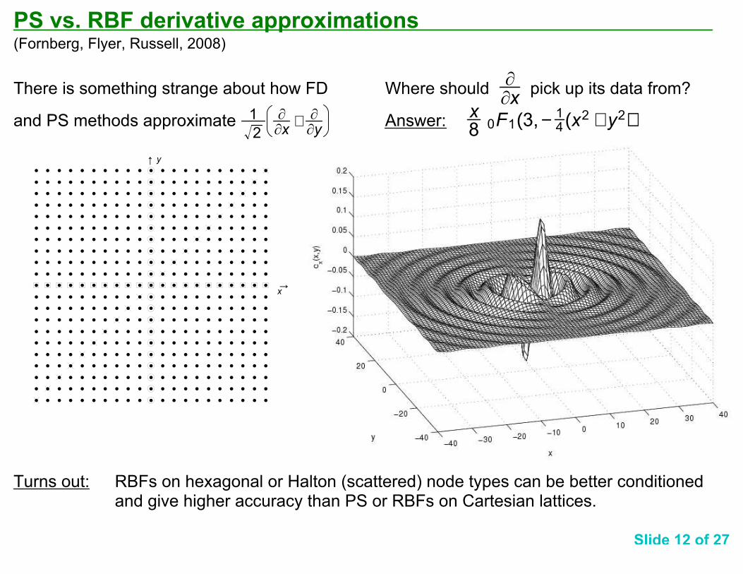
PS vs. RBF derivative approximations (Fornberg, Flyer, Russell, 2008)
There is something strange about how FD Where should pick up its data from?Ø
Øxand PS methods approximate Answer: 1
2
Ø
Øx+ ØØy
x8 0F1(3,− 1
4 (x2 + y2))
Turns out: RBFs on hexagonal or Halton (scattered) node types can be better conditionedand give higher accuracy than PS or RBFs on Cartesian lattices.
Slide 12 of 27
→x
↑ y
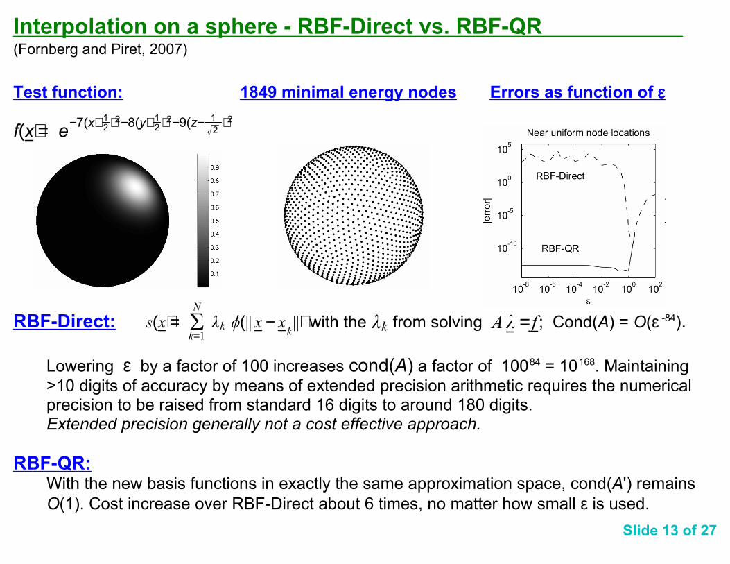
Interpolation on a sphere - RBF-Direct vs. RBF-QR (Fornberg and Piret, 2007)
Test function: 1849 minimal energy nodes Errors as function of εεεε
f(x) = e−7(x+ 12 )2−8(y+ 12 )2−9(z− 1
2)2
RBF-Direct: with the from solving ; Cond(A) = O(ε -84). s(x) = �k=1
N
�k �(|| x − xk||) �k A� = f
Lowering ε by a factor of 100 increases cond(A) a factor of 100
84 = 10
168. Maintaining
>10 digits of accuracy by means of extended precision arithmetic requires the numericalprecision to be raised from standard 16 digits to around 180 digits. Extended precision generally not a cost effective approach.
RBF-QR: With the new basis functions in exactly the same approximation space, cond(A') remains
O(1). Cost increase over RBF-Direct about 6 times, no matter how small ε is used.Slide 13 of 27
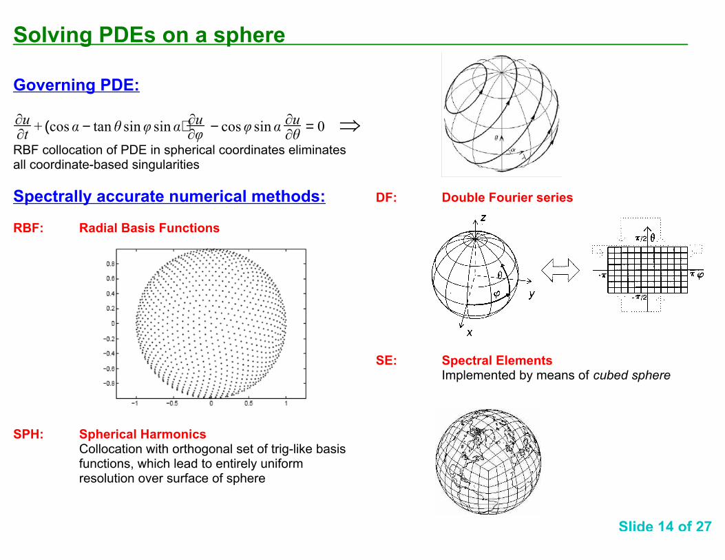
Solving PDEs on a sphere
Governing PDE:
⇒ØuØt
+ (cos � − tan � sin� sin �) ØuØ�
− cos� sin � ØuØ�
= 0
RBF collocation of PDE in spherical coordinates eliminatesall coordinate-based singularities
Spectrally accurate numerical methods: DF: Double Fourier series
RBF: Radial Basis Functions Below: 1849 minimum energy nodes
SE: Spectral ElementsImplemented by means of cubed sphere
SPH: Spherical HarmonicsCollocation with orthogonal set of trig-like basis functions, which lead to entirely uniformresolution over surface of sphere
Slide 14 of 27
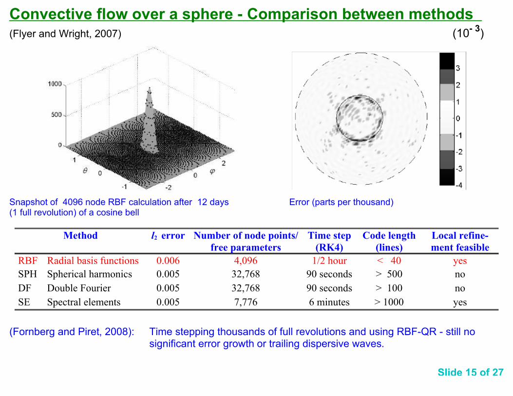
Convective flow over a sphere - Comparison between methods (Flyer and Wright, 2007) (10
- 3)
Snapshot of 4096 node RBF calculation after 12 days Error (parts per thousand)(1 full revolution) of a cosine bell
yes> 10006 minutes7,7760.005Spectral elementsSE
no> 10090 seconds32,7680.005Double FourierDF
no> 50090 seconds32,7680.005Spherical harmonicsSPH
yes< 401/2 hour4,0960.006Radial basis functionsRBF
Local refine-
ment feasible
Code length
(lines)
Time step
(RK4)
Number of node points/
free parameters
l2 errorMethod
(Fornberg and Piret, 2008): Time stepping thousands of full revolutions and using RBF-QR - still nosignificant error growth or trailing dispersive waves.
Slide 15 of 27
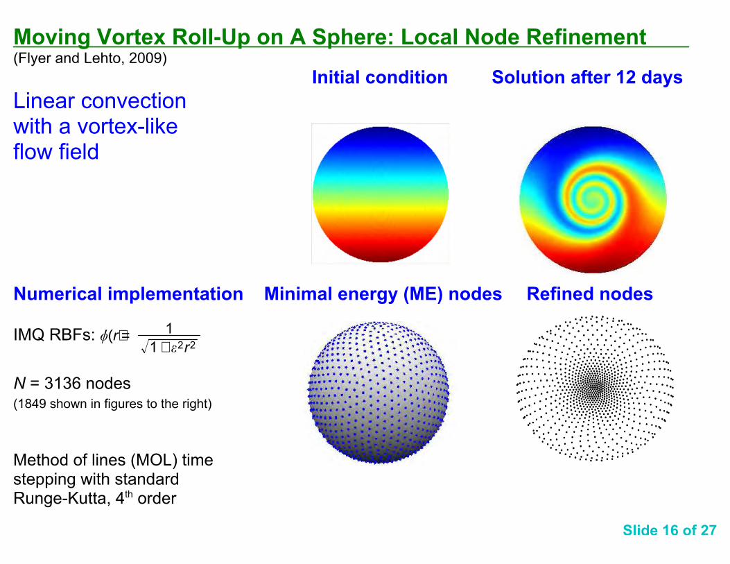
Moving Vortex Roll-Up on A Sphere: Local Node Refinement (Flyer and Lehto, 2009)
Initial condition Solution after 12 days
Linear convectionwith a vortex-likeflow field
Numerical implementation Minimal energy (ME) nodes Refined nodes
IMQ RBFs: �(r) = 1
1 + �2r2
N = 3136 nodes (1849 shown in figures to the right)
Method of lines (MOL) time stepping with standardRunge-Kutta, 4th order
Slide 16 of 27
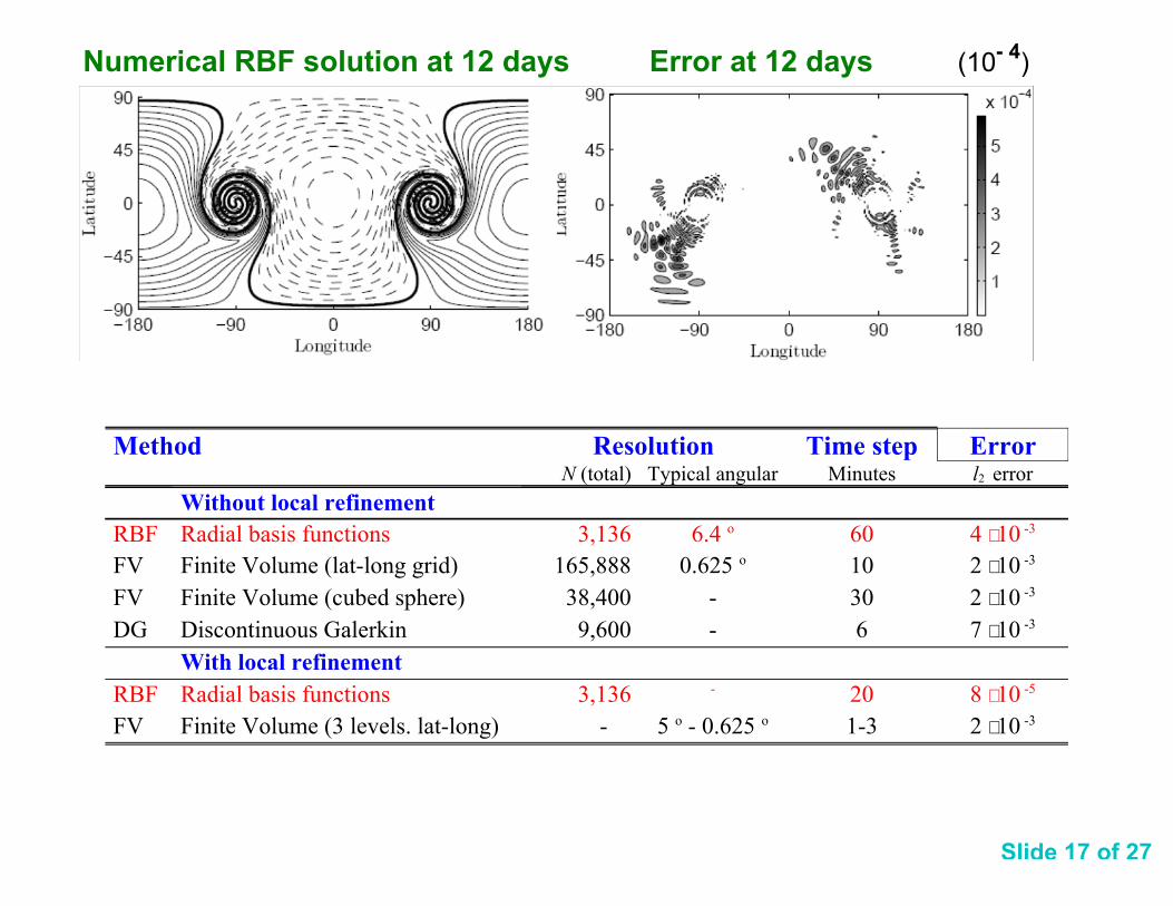
Numerical RBF solution at 12 days Error at 12 days (10- 4)
2 ⋅ 10 -31-35 o - 0.625 o- Finite Volume (3 levels. lat-long)FV
8 ⋅ 10 -520-3,136Radial basis functionsRBF
With local refinement
7 ⋅ 10 -36-9,600Discontinuous GalerkinDG
2 ⋅ 10 -330-38,400Finite Volume (cubed sphere)FV
2 ⋅ 10 -3100.625 o165,888Finite Volume (lat-long grid)FV
4 ⋅ 10 -3606.4 o3,136Radial basis functionsRBF
Without local refinement
l2 errorMinutesTypical angularN (total)
ErrorTime stepResolutionMethod
Slide 17 of 27
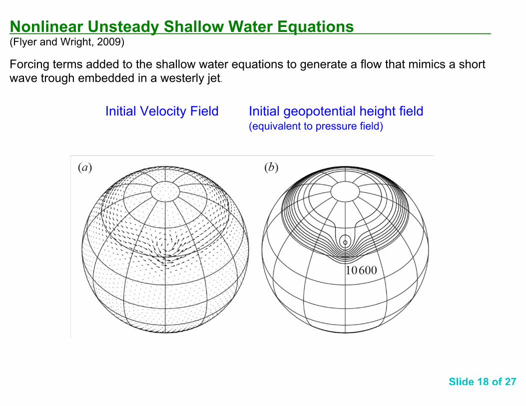
Nonlinear Unsteady Shallow Water Equations (Flyer and Wright, 2009)
Forcing terms added to the shallow water equations to generate a flow that mimics a shortwave trough embedded in a westerly jet.
Initial Velocity Field Initial geopotential height field(equivalent to pressure field)
Slide 18 of 27
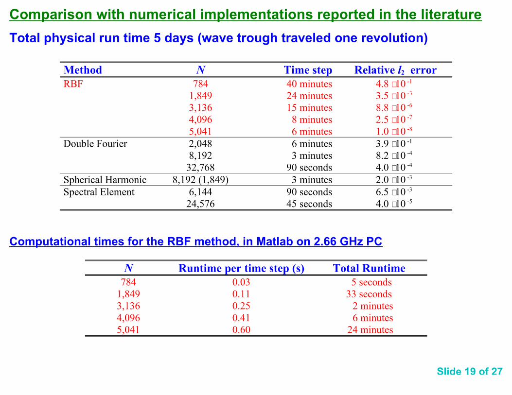
Comparison with numerical implementations reported in the literature
Total physical run time 5 days (wave trough traveled one revolution)
4.0 ⋅ 10 -545 seconds24,576
6.5 ⋅ 10 -390 seconds6,144Spectral Element
2.0 ⋅ 10 -33 minutes8,192 (1,849)Spherical Harmonic
4.0 ⋅ 10 -490 seconds32,768
8.2 ⋅ 10 -43 minutes8,192
3.9 ⋅ 10 -16 minutes2,048Double Fourier
1.0 ⋅ 10 -86 minutes5,041
2.5 ⋅ 10 -7 8 minutes4,096
8.8 ⋅ 10 -615 minutes3,136
3.5 ⋅ 10 -324 minutes1,849
4.8 ⋅ 10 -140 minutes784RBF
Relative l2 errorTime stepNMethod
Computational times for the RBF method, in Matlab on 2.66 GHz PC
24 minutes 0.605,041
6 minutes0.414,096
2 minutes0.253,136
33 seconds0.111,849
5 seconds 0.03784
Total RuntimeRuntime per time step (s)N
Slide 19 of 27
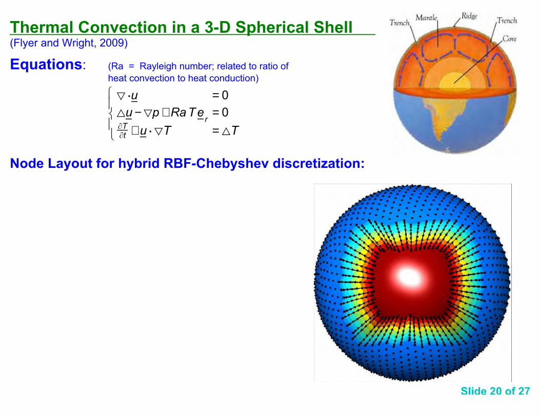
Thermal Convection in a 3-D Spherical Shell (Flyer and Wright, 2009)
Equations: (Ra = Rayleigh number; related to ratio of
heat convection to heat conduction)
= $u = 0<u −=p +RaTe
r= 0
ØTØt + u $ =T = <T
Node Layout for hybrid RBF-Chebyshev discretization:
Slide 20 of 27
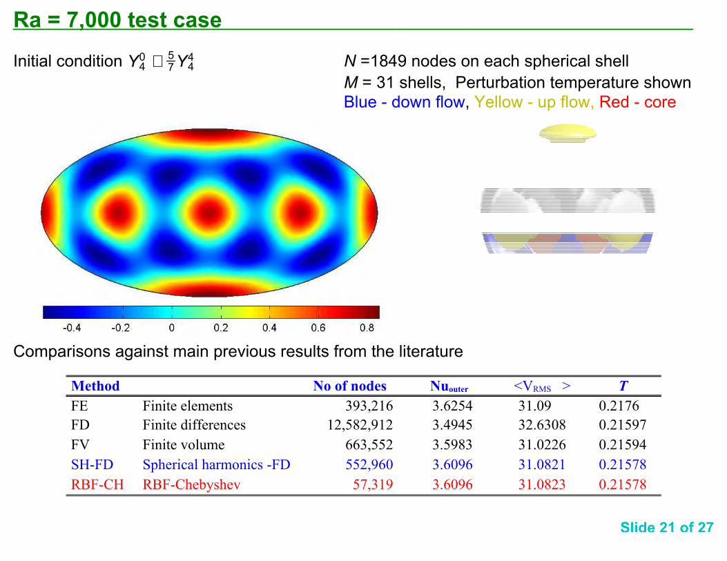
Ra = 7,000 test case
Initial condition N =1849 nodes on each spherical shellY40 + 5
7Y44
M = 31 shells, Perturbation temperature shown
Blue - down flow, Yellow - up flow, Red - core
Comparisons against main previous results from the literature
0.2157831.08233.6096 57,319RBF-ChebyshevRBF-CH
0.2157831.08213.6096 552,960Spherical harmonics -FDSH-FD
0.2159431.02263.5983 663,552Finite volumeFV
0.2159732.63083.4945 12,582,912Finite differencesFD
0.2176 31.09 3.6254 393,216Finite elementsFE
T<VRMS >NuouterNo of nodesMethod
Slide 21 of 27
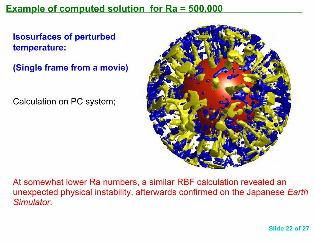
Example of computed solution for Ra = 500,000
Isosurfaces of perturbed
temperature:
(Single frame from a movie)
Calculation on PC system;
At somewhat lower Ra numbers, a similar RBF calculation revealed anunexpected physical instability, afterwards confirmed on the Japanese EarthSimulator.
Slide 22 of 27
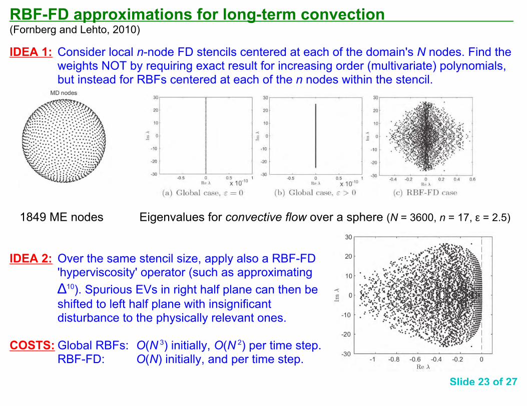
RBF-FD approximations for long-term convection (Fornberg and Lehto, 2010)
IDEA 1: Consider local n-node FD stencils centered at each of the domain's N nodes. Find theweights NOT by requiring exact result for increasing order (multivariate) polynomials,but instead for RBFs centered at each of the n nodes within the stencil.
1849 ME nodes Eigenvalues for convective flow over a sphere (N = 3600, n = 17, ε = 2.5)
IDEA 2: Over the same stencil size, apply also a RBF-FD'hyperviscosity' operator (such as approximating
∆10). Spurious EVs in right half plane can then be
shifted to left half plane with insignificantdisturbance to the physically relevant ones.
COSTS:Global RBFs: O(N 3) initially, O(N 2) per time step.RBF-FD: O(N) initially, and per time step.
Slide 23 of 27
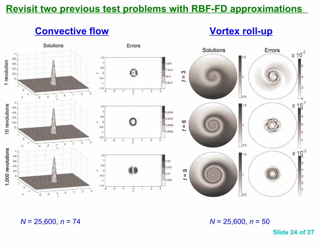
Revisit two previous test problems with RBF-FD approximations
Convective flow Vortex roll-up
N = 25,600, n = 74 N = 25,600, n = 50
Slide 24 of 27
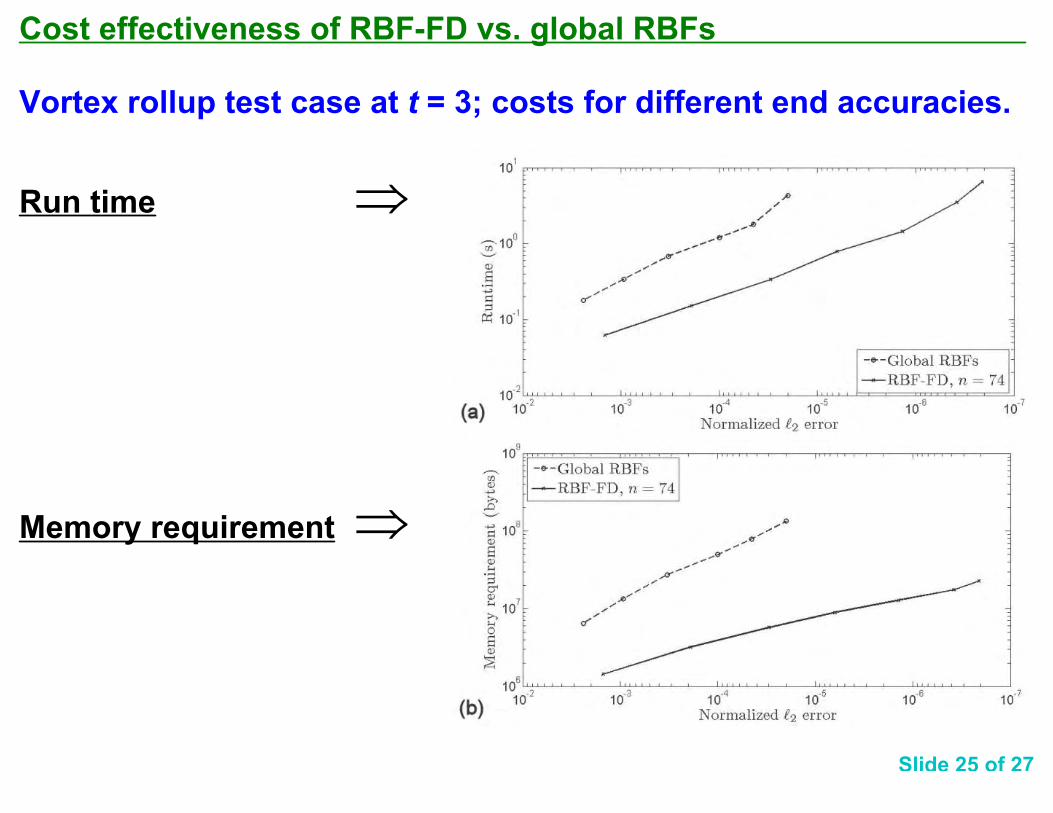
Cost effectiveness of RBF-FD vs. global RBFs
Vortex rollup test case at t = 3; costs for different end accuracies.
Run time ⇒
Memory requirement ⇒
Slide 25 of 27
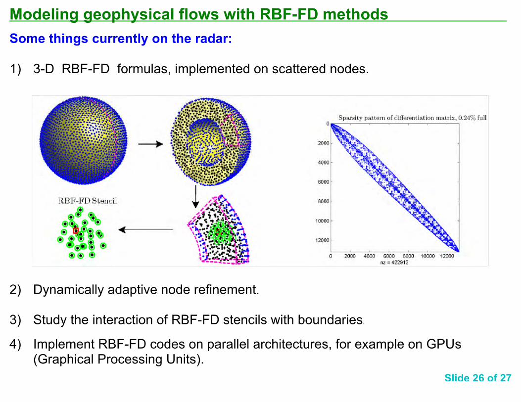
Modeling geophysical flows with RBF-FD methods
Some things currently on the radar:
1) 3-D RBF-FD formulas, implemented on scattered nodes.
2) Dynamically adaptive node refinement.
3) Study the interaction of RBF-FD stencils with boundaries.
4) Implement RBF-FD codes on parallel architectures, for example on GPUs(Graphical Processing Units).
Slide 26 of 27
Conclusions
Established:- RBFs can be seen as a generalization of PS methods to arbitrarily shaped domains.
- RBFs combine spectral accuracy with flexible opportunities for local node refinement.
- RBFs can offer excellent accuracy also over very long integration times.
- The near-flat basis function regime (ε small) is of particular interest, and stable numerical algorithmsfor it have been developed.
- For certain classes of convective flow problems, RBF-based solutions can be more accurate andcost-effective than any previous numerical method.
Some current research issues: - Develop further the RBF-FD approach.
- Compare both global RBFs and RBF-FD implementations against previous methods in more majorapplications.
- Explore further the combination of spectral accuracy with local node refinement.
- Try to find still more options for RBF algorithms that bypass all numerical instability issues.
- Develop effective implementations of RBF-FD methods, first on GPUs, and later on massively parallel(peta-scale) computer hardware.
References:- Flyer, N.and Fornberg, B., Radial basis functions: Developments and applications to planetary scale
flows, Computers and Fluids, in press.
- Fornberg, B. and Lehto, E., Stabilization of RBF-generated finite difference methods for convectivePDEs, submitted to J. Comput. Phys.
Slide 27 of 27


![Stability of traveling pulses with oscillatory tails in the FitzHugh ...€¦ · The oscillations in the tails were shown to arise along with a canard mechanism [22] in a local center](https://static.fdocument.org/doc/165x107/601a3ef0c68e6b5bec07f201/stability-of-traveling-pulses-with-oscillatory-tails-in-the-fitzhugh-the-oscillations.jpg)


![Hyat Huang , Jinbo Yang - arXiv · Black hole solutions can also arise from the EMD theories with the phantom dilaton. Gibbons and Rasheed [28] showed that there were massless black](https://static.fdocument.org/doc/165x107/5faa05f3503de154517d38c4/hyat-huang-jinbo-yang-arxiv-black-hole-solutions-can-also-arise-from-the-emd.jpg)