Radar radiation characteristics and measurements methods

Sara Adda

Arpa Piemonte – Physical and Technological Risks Department

Radar radiation characteristics

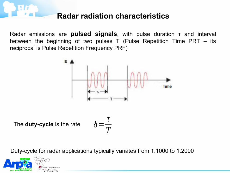
Radar emissions are pulsed signals, with pulse duration τ and interval between the beginning of two pulses T (Pulse Repetition Time PRT – its reciprocal is Pulse Repetition Frequency PRF)

The duty-cycle is the rate δ=τT

Duty-cycle for radar applications typically variates from 1:1000 to 1:2000

Antenna and radiation pattern features

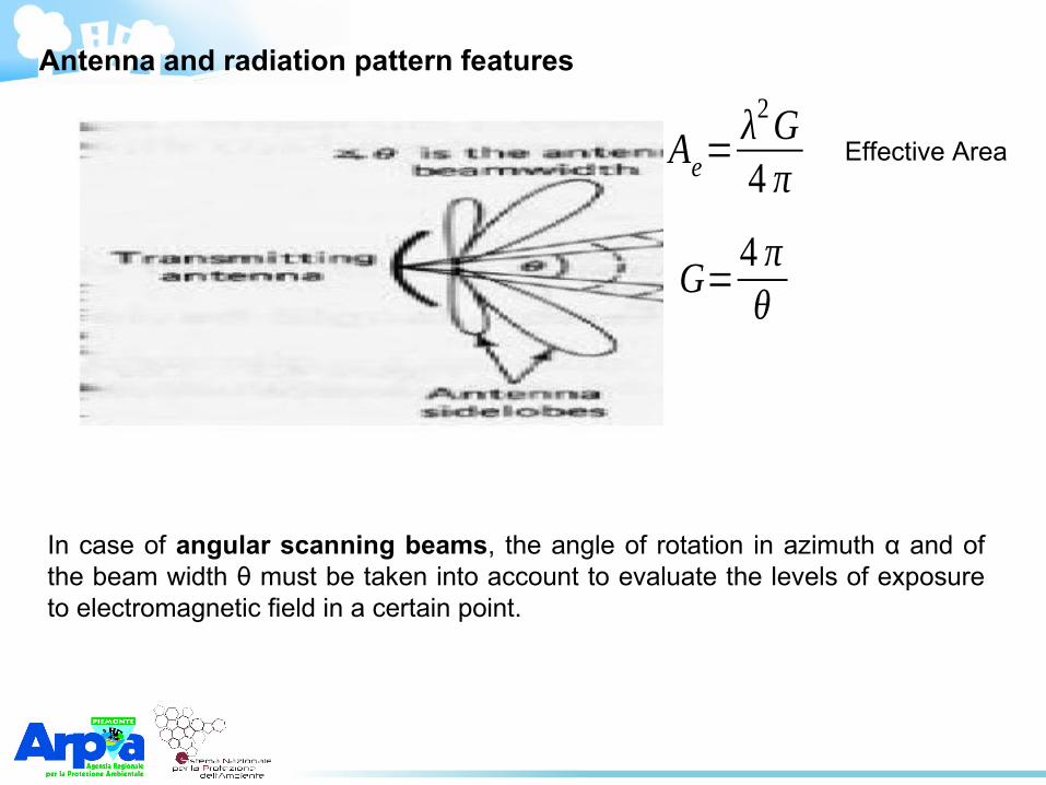
In case of angular scanning beams, the angle of rotation in azimuth α and of the beam width θ must be taken into account to evaluate the levels of exposure to electromagnetic field in a certain point.

Ae=λ2G4 π

Effective Area

G=4 πθ

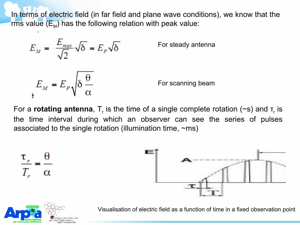
In terms of electric field (in far field and plane wave conditions), we know that the rms value (EM) has the following relation with peak value:

For steady antenna

For scanning beam

For a rotating antenna, Tr is the time of a single complete rotation (~s) and τr is the time interval during which an observer can see the series of pulses associated to the single rotation (illumination time, ~ms)

Visualisation of electric field as a function of time in a fixed observation point

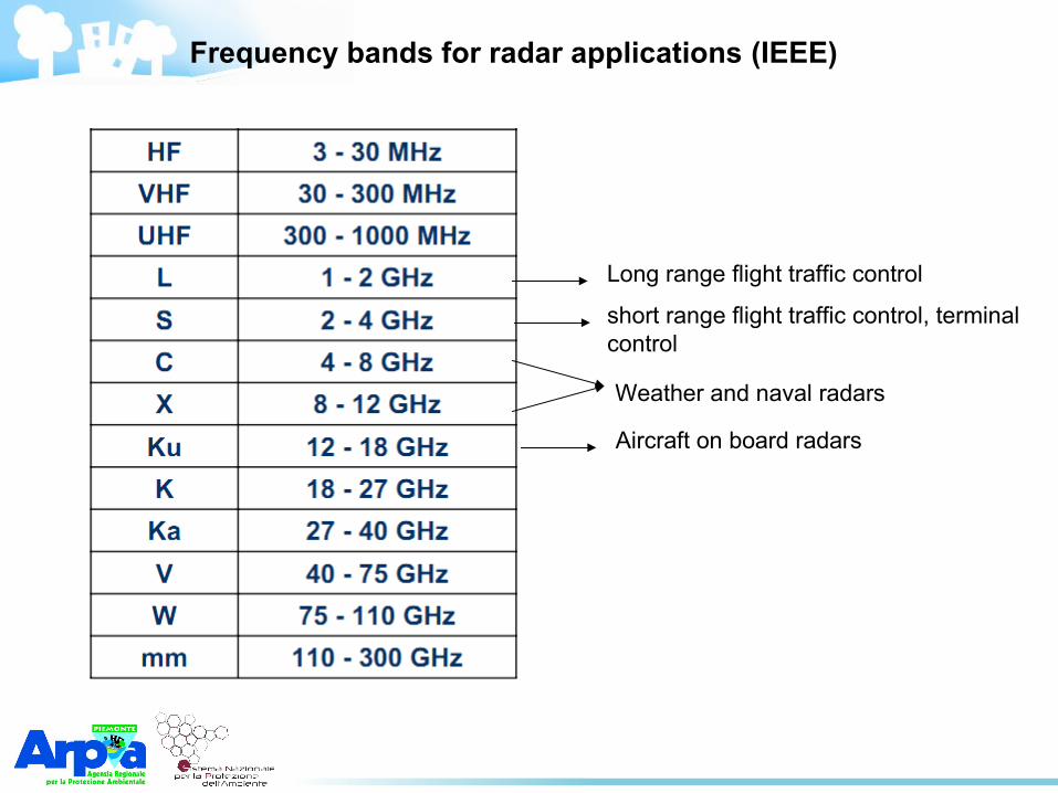
Frequency bands for radar applications (IEEE)

Long range flight traffic control

short range flight traffic control, terminal control

Weather and naval radars

Aircraft on board radars

Examples of radar characteristics

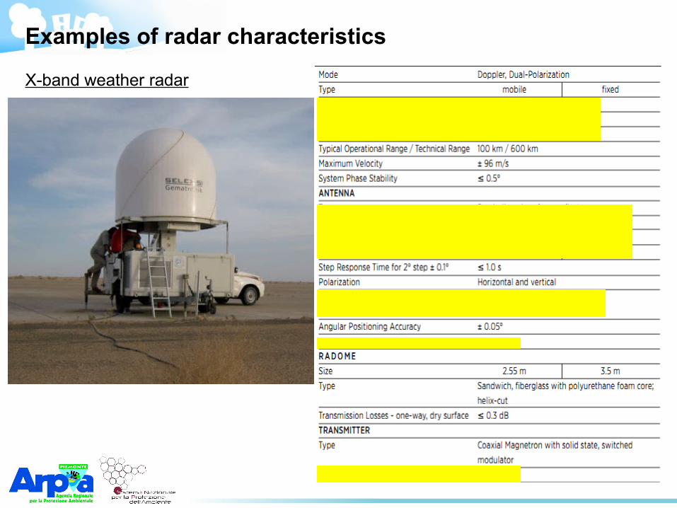
X-band weather radar

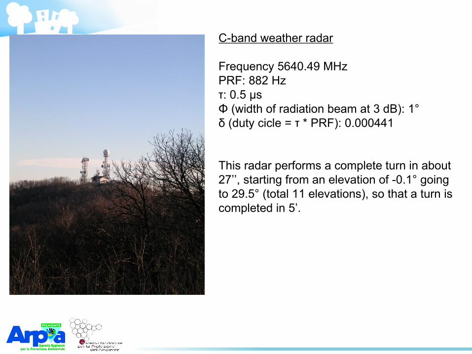
C-band weather radar

Frequency 5640.49 MHzPRF: 882 Hzτ: 0.5 μssΦ (width of radiation beam at 3 dB): 1°): 1°δ (duty cicle = τ * PRF): 0.000441

This radar performs a complete turn in about 27’’, starting from an elevation of -0.1° going to 29.5° (total 11 elevations), so that a turn is completed in 5’.

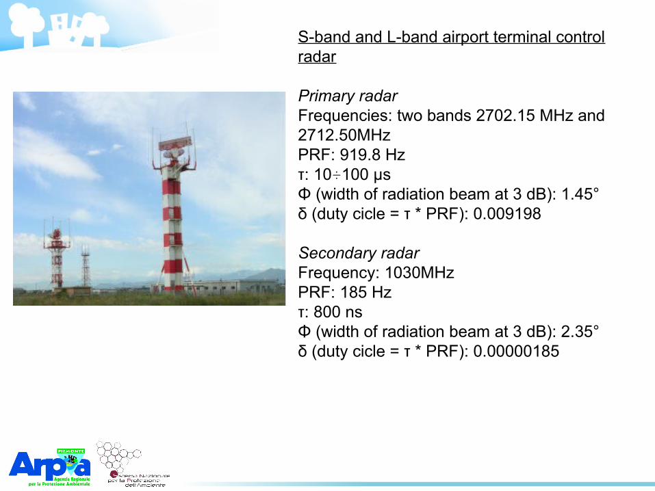
S-band and L-band airport terminal control radar

Primary radarFrequencies: two bands 2702.15 MHz and 2712.50MHzPRF: 919.8 Hzτ: 10÷100 μssΦ (width of radiation beam at 3 dB): 1°): 1.45°δ (duty cicle = τ * PRF): 0.009198

Secondary radarFrequency: 1030MHzPRF: 185 Hzτ: 800 nsΦ (width of radiation beam at 3 dB): 1°): 2.35°δ (duty cicle = τ * PRF): 0.00000185

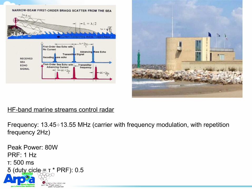
HF-band marine streams control radar

Frequency: 13.45÷13.55 MHz (carrier with frequency modulation, with repetition frequency 2Hz)

Peak Power: 80WPRF: 1 Hzτ: 500 msδ (duty cicle = τ * PRF): 0.5

Evaluating exposure to EMF from radar devices must take into account:

-Near field exposure: due to free field attenuation and great dimensions of transmitting antennas, risk zones usually are within the Fresnel radiative near field zone

-Pulse modulation: RF power is modulated with pulses during τ (typically about 1 μss), interspersed with rather long breaks (T, about 1 ms). The resulting duty cycle (τ/T)T) is quite low, so that the measuring instrument has to handle with very high peak values and quite low average values.

-Antenna rotation: the radiation beam of a rotating antenna illuminates a certain point every period of the antenna (typically about 10s.), for a time interval of about 10ms, so the signal to be measured has a periodic variation.

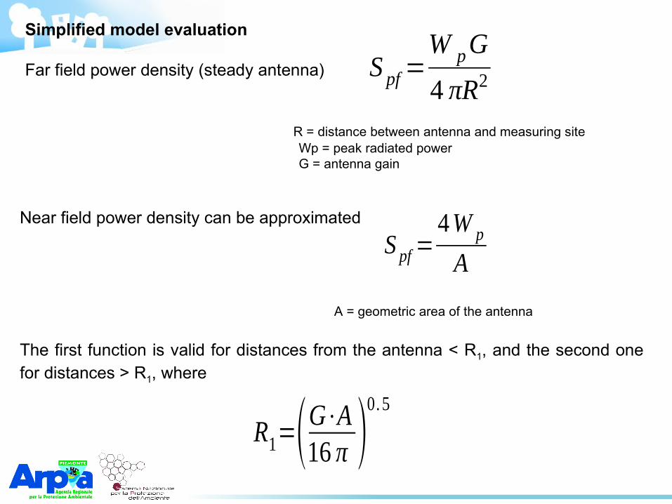
Simplified model evaluation

Far field power density (steady antenna)

R = distance between antenna and measuring site Wp = peak radiated power G = antenna gain

S pf=W pG

4 πR2

Near field power density can be approximated

A = geometric area of the antenna

S pf=4W p

A

The first function is valid for distances from the antenna < R1, and the second one for distances > R1, where

R1=(G⋅A16 π )

0. 5

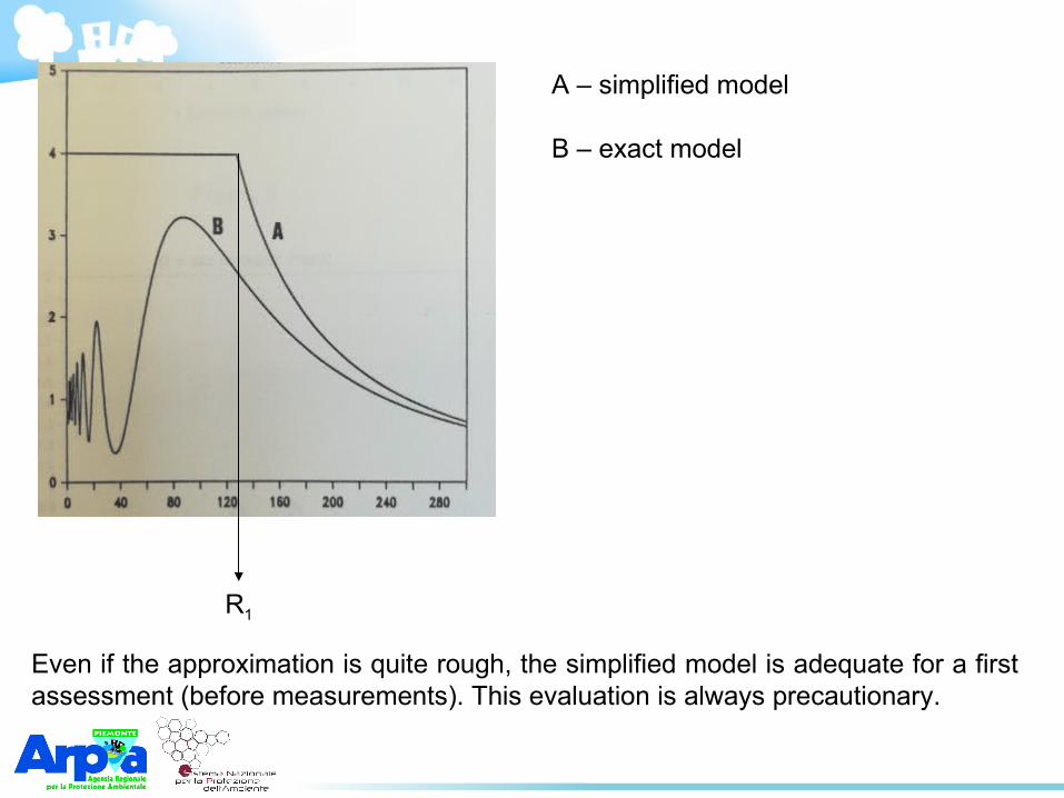
R1

A – simplified model

B): 1° – exact model

Even if the approximation is quite rough, the simplified model is adequate for a first assessment (before measurements). This evaluation is always precautionary.

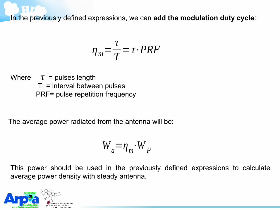
In the previously defined expressions, we can add the modulation duty cycle:

ηm=τT

=τ⋅PRF

Where = pulses length T = interval between pulses PRF= pulse repetition frequency

τ

The average power radiated from the antenna will be:

W a=ηm⋅W P

This power should be used in the previously defined expressions to calculate average power density with steady antenna.

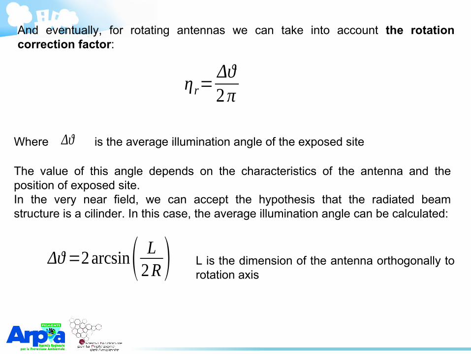
And eventually, for rotating antennas we can take into account the rotation correction factor:

ηr=Δϑ2π

Where is the average illumination angle of the exposed siteΔϑ

The value of this angle depends on the characteristics of the antenna and the position of exposed site.In the very near field, we can accept the hypothesis that the radiated beam structure is a cilinder. In this case, the average illumination angle can be calculated:

Δϑ=2 arcsin( L2R) L is the dimension of the antenna orthogonally to rotation axis

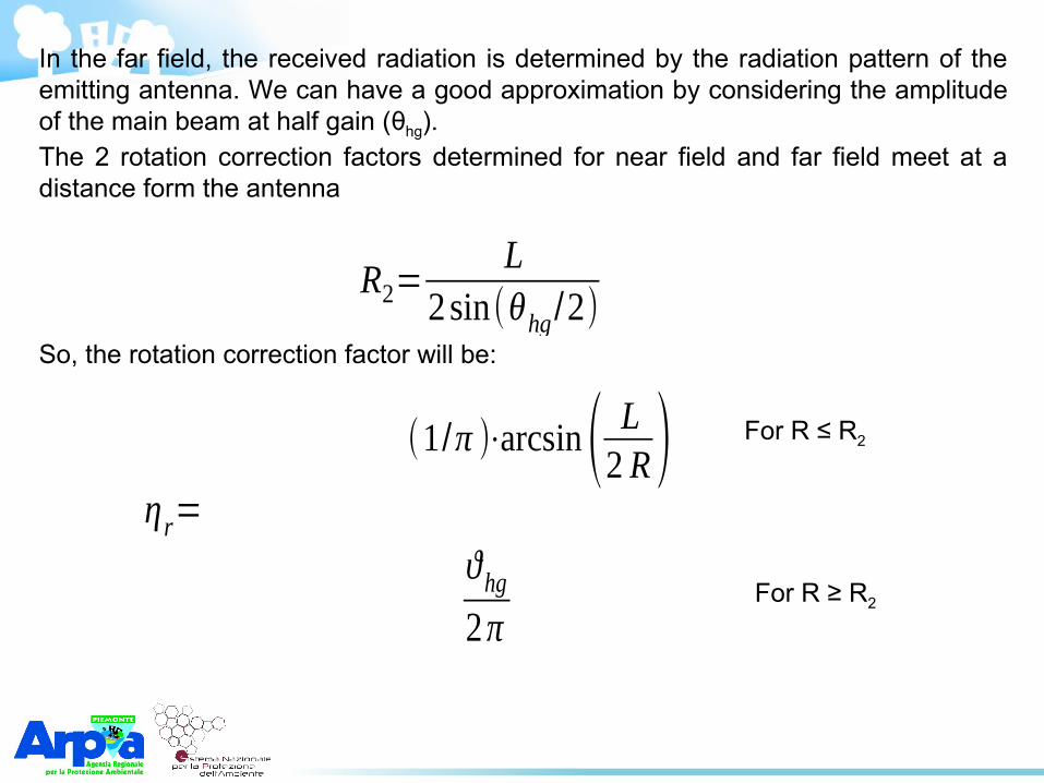
In the far field, the received radiation is determined by the radiation pattern of the emitting antenna. We can have a good approximation by considering the amplitude of the main beam at half gain (θhg).The 2 rotation correction factors determined for near field and far field meet at a distance form the antenna

R2=L

2sin(θhg /2)So, the rotation correction factor will be:

(1/π )⋅arcsin( L2 R)ηr=

ϑhg2π

For R ≤ R2

For R ≥ R2

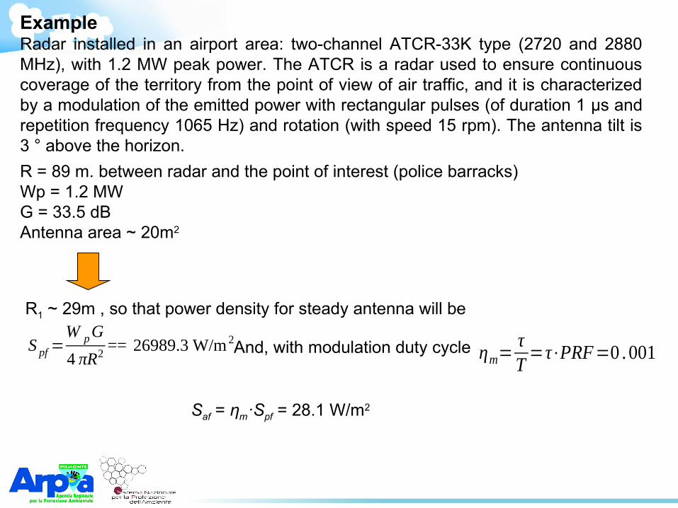
ExampleRadar installed in an airport area: two-channel ATCR-33K type (2720 and 2880 MHz), with 1.2 MW peak power. The ATCR is a radar used to ensure continuous coverage of the territory from the point of view of air traffic, and it is characterized by a modulation of the emitted power with rectangular pulses (of duration 1 μss and repetition frequency 1065 Hz) and rotation (with speed 15 rpm). The antenna tilt is 3 ° above the horizon.

R = 89 m. between radar and the point of interest (police barracks)Wp = 1.2 MWG = 33.5 dB): 1° Antenna area ~ 20m2

R1 ~ 29m , so that power density for steady antenna will be

S pf=W pG

4 πR2== 26989.3 W/m 2

ηm=τT

=τ⋅PRF=0 . 001And, with modulation duty cycle

Saf = ηm·Spf = 28.1 W/T)m2

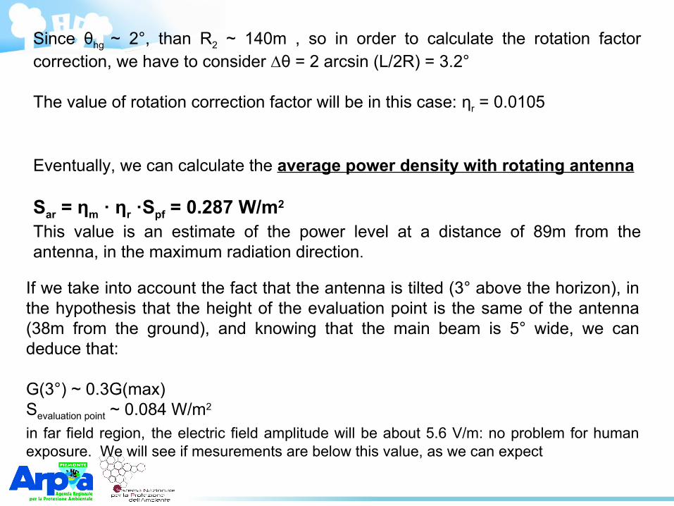
Since θhg ~ 2°, than R2 ~ 140m , so in order to calculate the rotation factor correction, we have to consider ∆θ = 2 arcsin (L/T)2R) = 3.2°

The value of rotation correction factor will be in this case: ηr = 0.0105

Eventually, we can calculate the average power density with rotating antenna

Sar = ηm · ηr ·Spf = 0.287 W/m2 This value is an estimate of the power level at a distance of 89m from the antenna, in the maximum radiation direction.

If we take into account the fact that the antenna is tilted (3° above the horizon), in the hypothesis that the height of the evaluation point is the same of the antenna (38m from the ground), and knowing that the main beam is 5° wide, we can deduce that:

G(3°) ~ 0.3G(max)Sevaluation point ~ 0.084 W/T)m2

in far field region, the electric field amplitude will be about 5.6 V/T)m: no problem for human exposure. We will see if mesurements are below this value, as we can expect

Measurements: what?

In order to perform comparison with exposure limits, we need to know:

Working frequency

Average power density or Electric field (RMS value)

Peak power density or Electric field

Other parameters that can be detected (for further verification):

Pulse Repetition Time

Rotation Time

Pulse length

Illumination Time

Measurements: which instruments?

Wideband instruments with diode sensors: necessary to check if the response is adequate to the pulse signals, and to estimate the associated uncertainty

Receiving antenna connected to:

Spectrum Analyser : it can be used in Pulse Spectrum Mode, Channel Power Mode or Span Zero Mode (time domain measurements)

Diode detector and oscilloscope: completely time-domain measurements, doesn’t allow working frequency detection.

Measuring radar signals with diode sensors (wideband instruments)

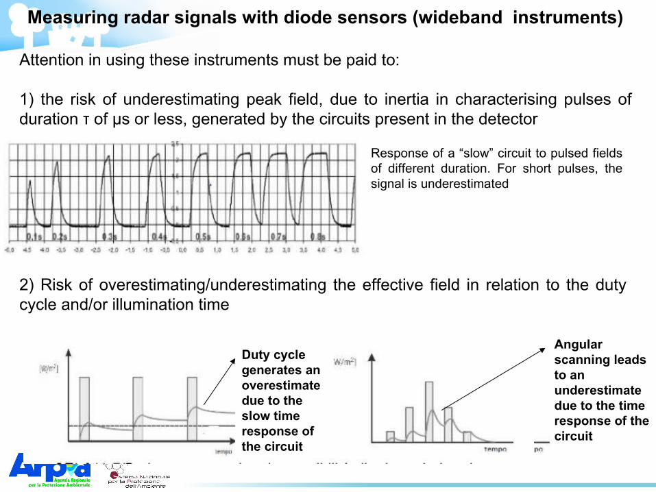
Attention in using these instruments must be paid to:

1) the risk of underestimating peak field, due to inertia in characterising pulses of duration τ of µs or less, generated by the circuits present in the detector

Response of a “slow” circuit to pulsed fields of different duration. For short pulses, the signal is underestimated

2) Risk of overestimating/T)underestimating the effective field in relation to the duty cycle and/T)or illumination time

Duty cycle generates an overestimate due to the slow time response of the circuit

Angular scanning leads to an underestimate due to the time response of the circuit

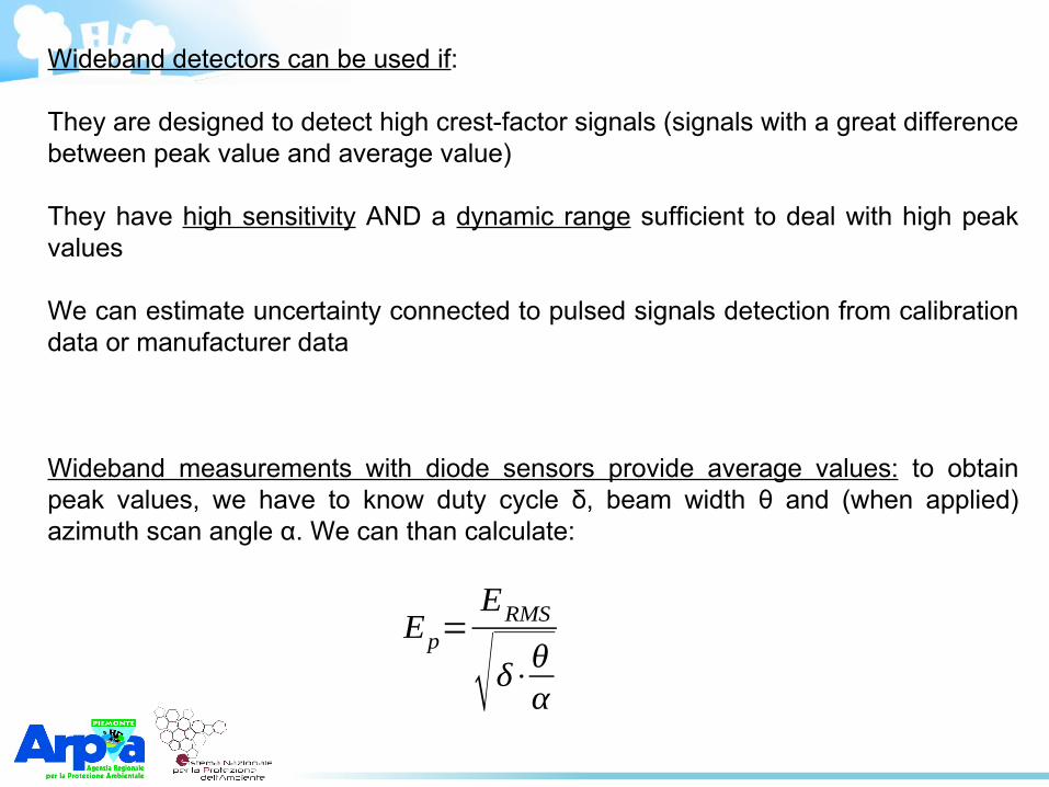
Wideband detectors can be used if:

They are designed to detect high crest-factor signals (signals with a great difference between peak value and average value)

They have high sensitivity AND a dynamic range sufficient to deal with high peak values

We can estimate uncertainty connected to pulsed signals detection from calibration data or manufacturer data

Wideband measurements with diode sensors provide average values: to obtain peak values, we have to know duty cycle δ, beam width θ and (when applied) azimuth scan angle α. We can than calculate:

Ep=ERMS

√δ⋅θα

Measuring radar signals with spectrum analyser

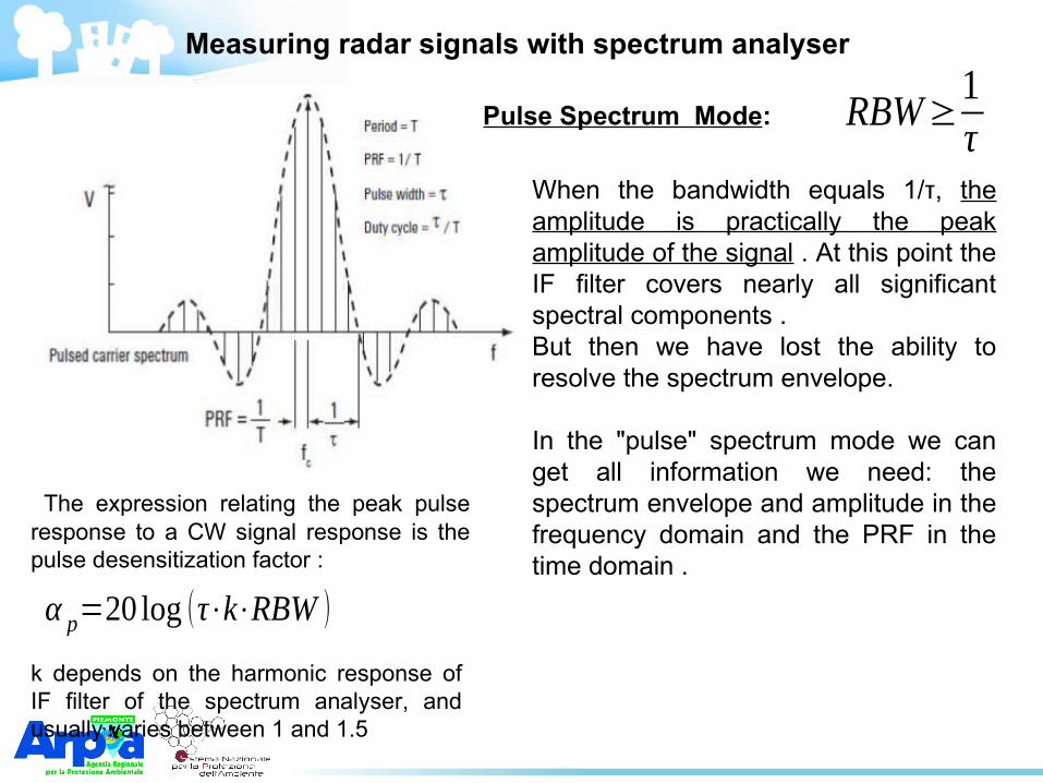
Pulse Spectrum Mode: RBW≥1τ

The expression relating the peak pulse response to a CW signal response is the pulse desensitization factor :

α p=20 log (τ⋅k⋅RBW )

k depends on the harmonic response of IF filter of the spectrum analyser, and usually varies between 1 and 1.5

When the bandwidth equals 1/T)τ, the amplitude is practically the peak amplitude of the signal . At this point the IF filter covers nearly all significant spectral components .B): 1°ut then we have lost the ability to resolve the spectrum envelope.

In the "pulse" spectrum mode we can get all information we need: the spectrum envelope and amplitude in the frequency domain and the PRF in the time domain .

Other parameters:

Peak detector

VB): 1°W≥RB): 1°W

SPAN ~ 3-4 times 1/T)τ

Measuring radar signals with spectrum analyser

Peak power

Measuring radar signals with spectrum analyser

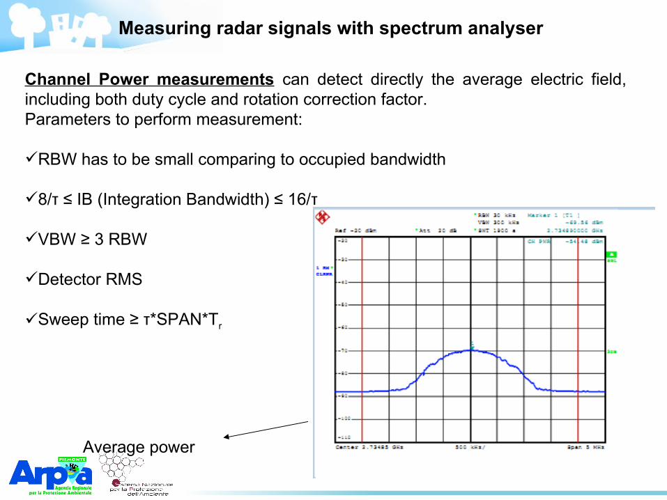
Channel Power measurements can detect directly the average electric field, including both duty cycle and rotation correction factor.Parameters to perform measurement:

RB): 1°W has to be small comparing to occupied bandwidth

8/T)τ ≤ IB): 1° (Integration B): 1°andwidth) ≤ 16/T)τ

VB): 1°W ≥ 3 RB): 1°W

Detector RMS

Sweep time ≥ τ*SPAN*Tr

Average power

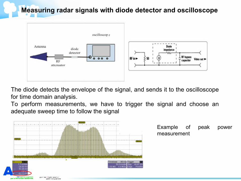
Measuring radar signals with diode detector and oscilloscope

The diode detects the envelope of the signal, and sends it to the oscilloscope for time domain analysis.To perform measurements, we have to trigger the signal and choose an adequate sweep time to follow the signal

Example of peak power measurement

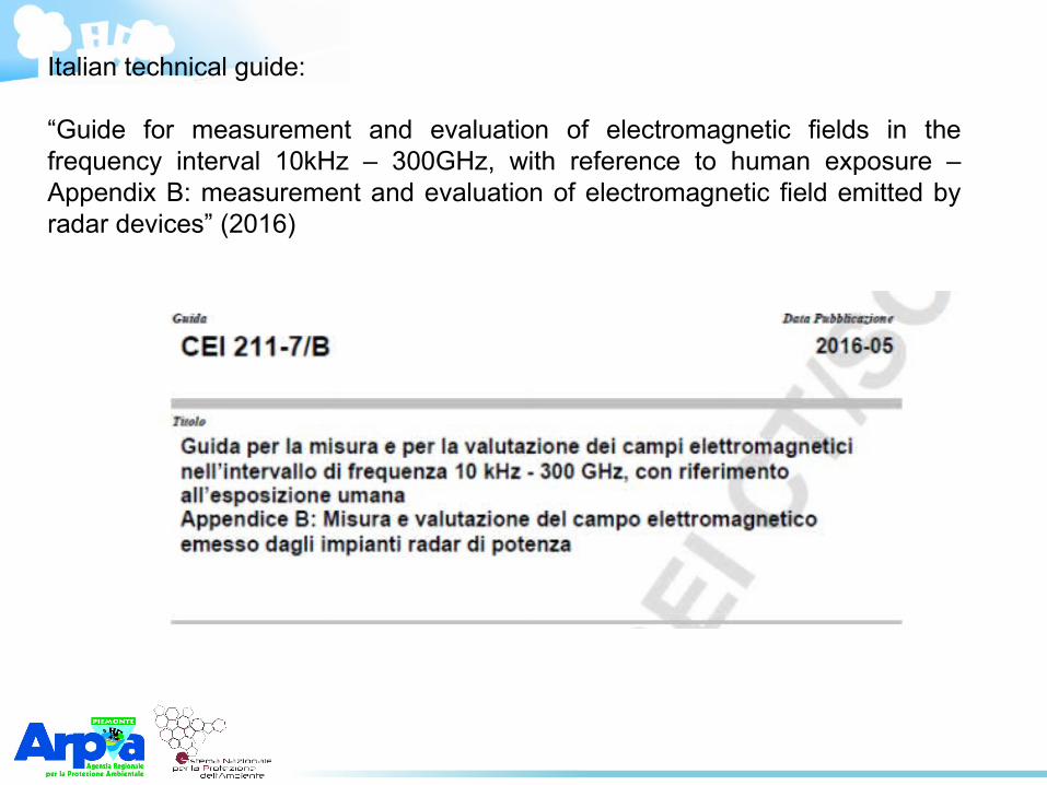
Italian technical guide:

“Guide for measurement and evaluation of electromagnetic fields in the frequency interval 10kHz – 300GHz, with reference to human exposure – Appendix B): 1°: measurement and evaluation of electromagnetic field emitted by radar devices” (2016)

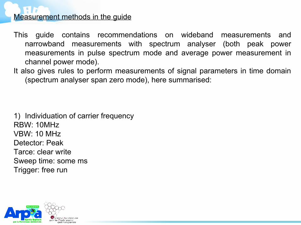
Measurement methods in the guide

This guide contains recommendations on wideband measurements and narrowband measurements with spectrum analyser (both peak power measurements in pulse spectrum mode and average power measurement in channel power mode).

It also gives rules to perform measurements of signal parameters in time domain (spectrum analyser span zero mode), here summarised:

1) Individuation of carrier frequencyRB): 1°W: 10MHzVB): 1°W: 10 MHzDetector: PeakTarce: clear writeSweep time: some msTrigger: free run

Measurement methods in the guide

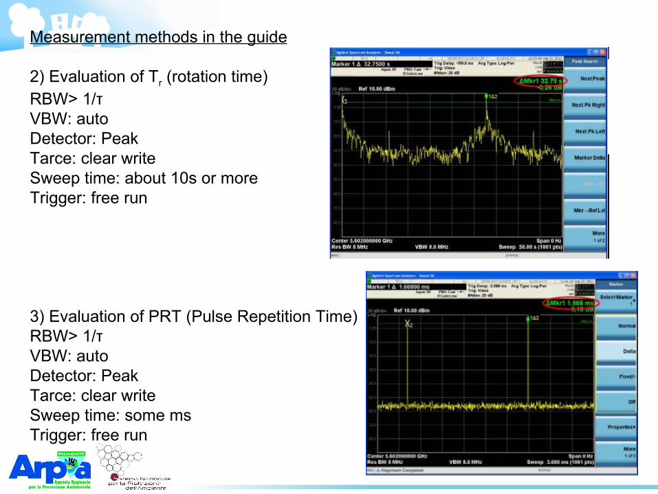
2) Evaluation of Tr (rotation time)RB): 1°W> 1/T)τVB): 1°W: autoDetector: PeakTarce: clear writeSweep time: about 10s or moreTrigger: free run

3) Evaluation of PRT (Pulse Repetition Time)RB): 1°W> 1/T)τVB): 1°W: autoDetector: PeakTarce: clear writeSweep time: some msTrigger: free run

Measurement methods in the guide

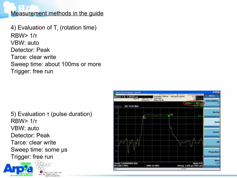
4) Evaluation of Tr (rotation time)RB): 1°W> 1/T)τVB): 1°W: autoDetector: PeakTarce: clear writeSweep time: about 100ms or moreTrigger: free run

5) Evaluation τ (pulse duration)RB): 1°W> 1/T)τVB): 1°W: autoDetector: PeakTarce: clear writeSweep time: some µsTrigger: free run

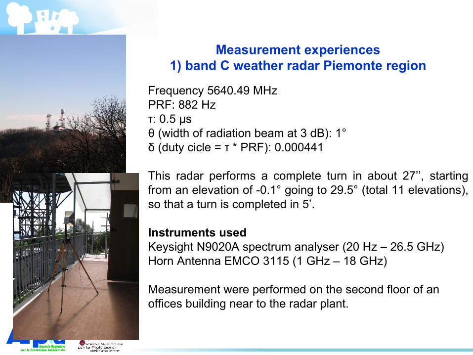
Measurement experiences1) band C weather radar Piemonte region

Frequency 5640.49 MHzPRF: 882 Hzτ: 0.5 μssθ (width of radiation beam at 3 dB): 1°): 1°δ (duty cicle = τ * PRF): 0.000441

This radar performs a complete turn in about 27’’, starting from an elevation of -0.1° going to 29.5° (total 11 elevations), so that a turn is completed in 5’.

Instruments usedKeysight N9020A spectrum analyser (20 Hz – 26.5 GHz)Horn Antenna EMCO 3115 (1 GHz – 18 GHz)

Measurement were performed on the second floor of an offices building near to the radar plant.

Analyser parameters Standard Chosen parameter

RBW 1/ττ 4 MHz

VBW 10RBWRBW 50RBW MHz

Span 3-4 (1/ττ) 10RBW MHz

Detector peak Peak

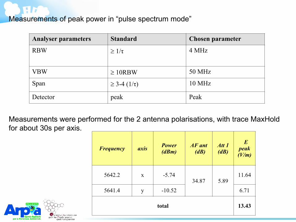
Measurements of peak power in “pulse spectrum mode”

Measurements were performed for the 2 antenna polarisations, with trace MaxHold for about 30s per axis.

Frequency axis Power(dBm)

AF ant (dB)

Att 1(dB)

E peak(V/m)

5642.2 x -5.7434.87 5.89

11.64

5641.4 y -10RBW.52 6.71

total 13.43

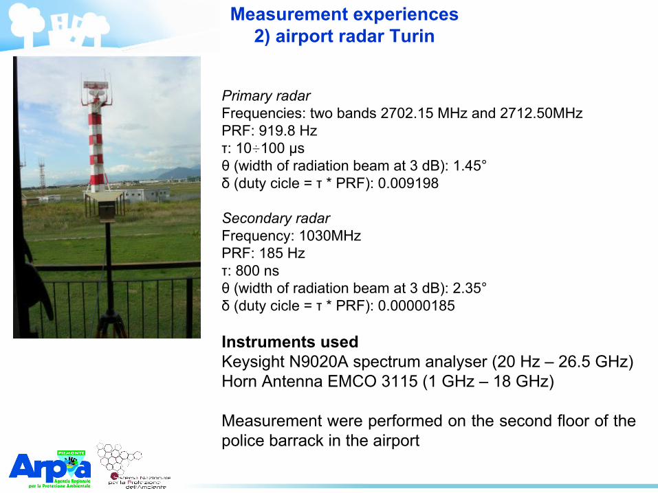
Measurement experiences2) airport radar Turin

Primary radarFrequencies: two bands 2702.15 MHz and 2712.50MHzPRF: 919.8 Hzτ: 10÷100 μssθ (width of radiation beam at 3 dB): 1°): 1.45°δ (duty cicle = τ * PRF): 0.009198

Secondary radarFrequency: 1030MHzPRF: 185 Hzτ: 800 nsθ (width of radiation beam at 3 dB): 1°): 2.35°δ (duty cicle = τ * PRF): 0.00000185

Instruments usedKeysight N9020A spectrum analyser (20 Hz – 26.5 GHz)Horn Antenna EMCO 3115 (1 GHz – 18 GHz)

Measurement were performed on the second floor of the police barrack in the airport

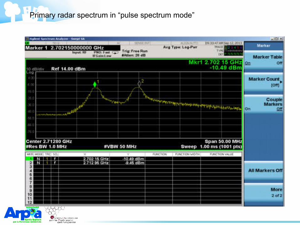
Primary radar spectrum in “pulse spectrum mode”

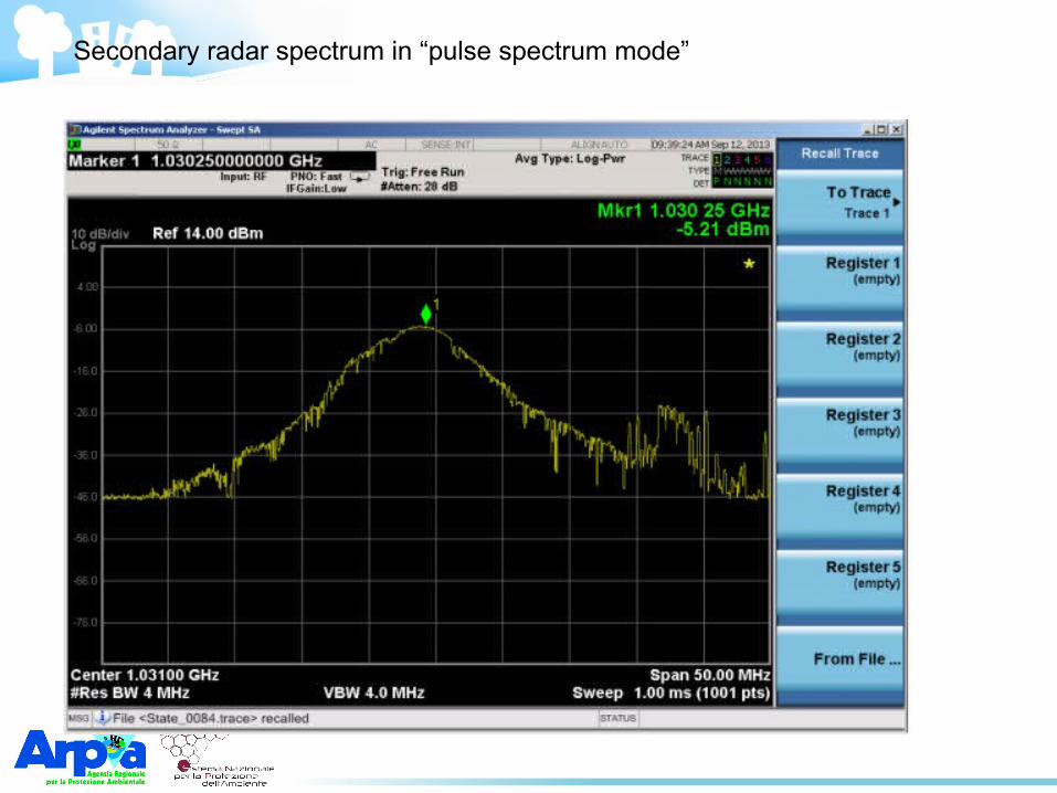
Secondary radar spectrum in “pulse spectrum mode”

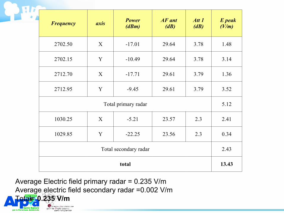
Frequency axisPower(dBm)

AF ant (dB)

Att 1(dB)

E peak(V/m)

270RBW2.50RBW X -17.0RBW1 29.64 3.78 1.48

270RBW2.15 Y -10RBW.49 29.64 3.78 3.14

2712.70RBW X -17.71 29.61 3.79 1.36

2712.95 Y -9.45 29.61 3.79 3.52

Total primary radar 5.12

10RBW30RBW.25 X -5.21 23.57 2.3 2.41

10RBW29.85 Y -22.25 23.56 2.3 0RBW.34

Total secondary radar 2.43

total 13.43

Average Electric field primary radar = 0.235 V/T)mAverage electric field secondary radar =0.002 V/T)mTotal= 0.235 V/m

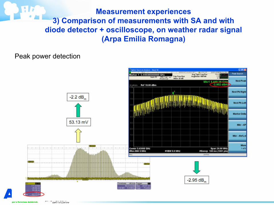
Measurement experiences3) Comparison of measurements with SA and with

diode detector + oscilloscope, on weather radar signal (Arpa Emilia Romagna)

Peak power detection

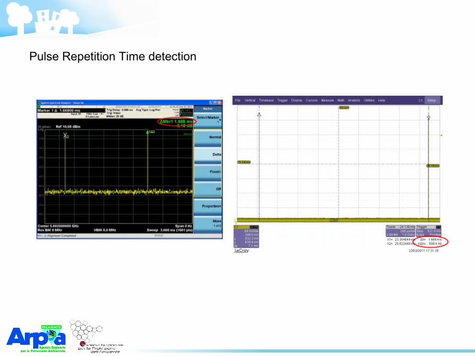
Pulse Repetition Time detection

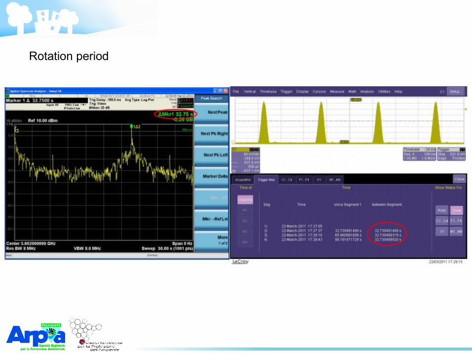
Rotation period

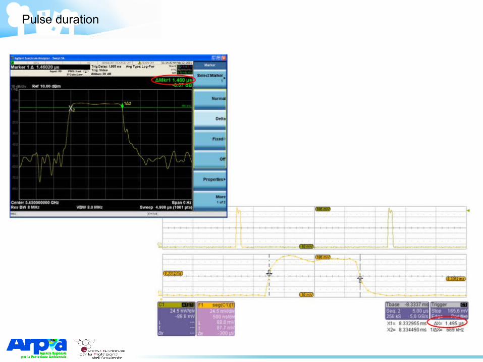
Pulse duration

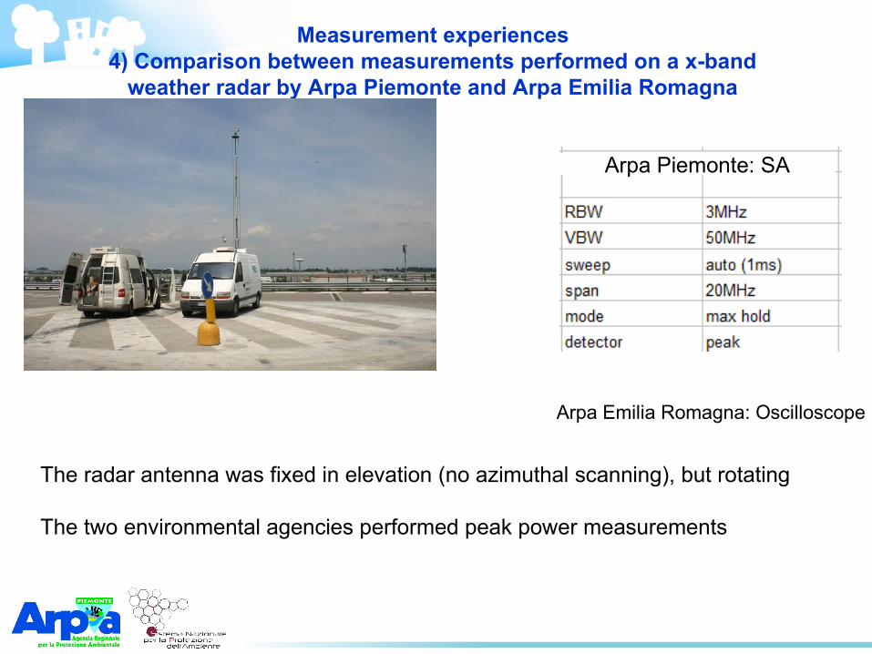
Measurement experiences4) Comparison between measurements performed on a x-band

weather radar by Arpa Piemonte and Arpa Emilia Romagna

Arpa Piemonte: SA

Arpa Emilia Romagna: Oscilloscope

The radar antenna was fixed in elevation (no azimuthal scanning), but rotating

The two environmental agencies performed peak power measurements

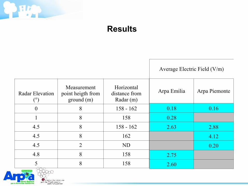
Radar Elevation (°)

Measurement point heigth from

ground (m)

Horizontal distance from

Radar (m)

0RBW 8 158 - 162

1 8 158

4.5 8 158 - 162

4.5 8 162

4.5 2 ND

4.8 8 158

5 8 158

Average Electric Field (V/τm)

Arpa Emilia Arpa Piemonte

0RBW.18 0RBW.16

0RBW.28

2.63 2.88

4.12

0RBW.20RBW

2.75

2.60RBW

Results

Thank you