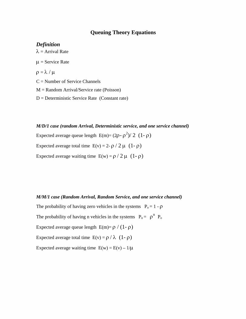
Queuing Theory Equations Definition λ = Arrival Rate

μ = Service Rate

ρ = λ / μ C = Number of Service Channels

M = Random Arrival/Service rate (Poisson)

D = Deterministic Service Rate (Constant rate)

M/D/1 case (random Arrival, Deterministic service, and one service channel)

Expected average queue length E(m)= (2ρ- ρ2)/ 2 (1- ρ)

Expected average total time E(v) = 2- ρ / 2 μ (1- ρ)

Expected average waiting time E(w) = ρ / 2 μ (1- ρ)

M/M/1 case (Random Arrival, Random Service, and one service channel)

The probability of having zero vehicles in the systems Po = 1 - ρ

The probability of having n vehicles in the systems Pn = ρn Po

Expected average queue length E(m)= ρ / (1- ρ)

Expected average total time E(v) = ρ / λ (1- ρ)

Expected average waiting time E(w) = E(v) – 1/μ

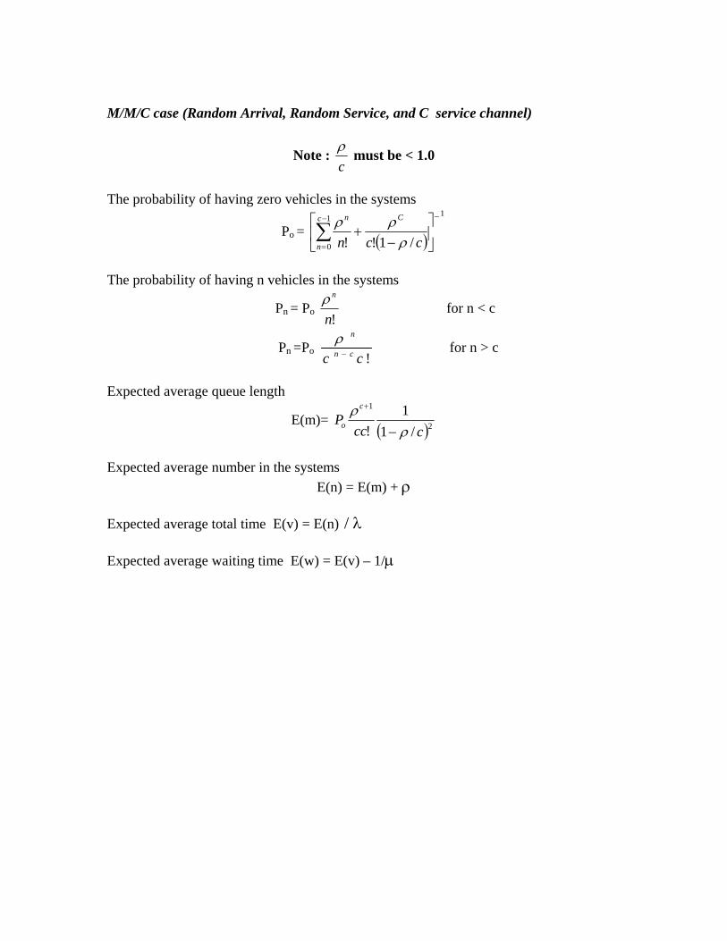
M/M/C case (Random Arrival, Random Service, and C service channel)

Note : cρ must be < 1.0

The probability of having zero vehicles in the systems

Po = ( )

1_1

0 /1!! ⎥⎦

⎤⎢⎣

⎡−

+∑−

=

c

n

Cn

ccn ρρρ

The probability of having n vehicles in the systems

Pn = Po !n

nρ for n < c

Pn =Po !cc cn

n

−

ρ for n > c

Expected average queue length

E(m)= ( )2

1

/11

! cccP

c

o ρρ

−

+

Expected average number in the systems

E(n) = E(m) + ρ Expected average total time E(v) = E(n) / λ Expected average waiting time E(w) = E(v) – 1/μ

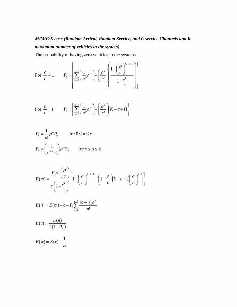
M/M/C/K case (Random Arrival, Random Service, and C service Channels and K

maximum number of vehicles in the system)

The probability of having zero vehicles in the systems

For 1≠cρ

1

1

0

1

1

1

!!1

−

−

=

+−

⎥⎥⎥⎥⎥

⎦

⎤

⎢⎢⎢⎢⎢

⎣

⎡

⎟⎟⎟⎟⎟

⎠

⎞

⎜⎜⎜⎜⎜

⎝

⎛

−

⎟⎠⎞

⎜⎝⎛−

⎟⎟⎠

⎞⎜⎜⎝

⎛+⎟⎠⎞

⎜⎝⎛= ∑

c

n

cK

cn

o

c

ccn

P ρ

ρρρ

For 1=cρ ( )

11

01

!!1

−−

=⎥⎦

⎤⎢⎣

⎡+−⎟⎟

⎠

⎞⎜⎜⎝

⎛+⎟⎠⎞

⎜⎝⎛= ∑

c

n

cn

o cKcn

P ρρ

cn0for !

1≤≤= o

nn P

nP ρ

kncfor P !c

1o

nc-n ≤≤⎟

⎠⎞

⎜⎝⎛= ρ

cPn

( )⎥⎥⎦

⎤

⎢⎢⎣

⎡⎟⎠⎞

⎜⎝⎛+−⎟

⎠⎞

⎜⎝⎛ −−⎟

⎠⎞

⎜⎝⎛−

⎟⎠⎞

⎜⎝⎛ −

⎟⎠⎞

⎜⎝⎛

=−+− ckck

co

cck

ccc

c

cP

mE ρρρρ

ρρ111

1!)(

1

2

∑−

=

−−+=

1

0 !)()()(

c

n

n

o nncPcmEnE ρ

( )KPnEvE−

=1

)()(λ

μ1)()( −= vEwE