QUASI-STATIC AND DYNAMIC COMPACTION OF POROUS …

12 March 2010Yehuda Partom1

QUASI-STATIC AND DYNAMIC COMPACTION OF POROUS MATERIALS

Yehuda Partom

RAFAEL, Haifa, ISRAEL

‘From Static to dynamic’, London, 22-23 February 2010.


Outline

Herrmann’s EOS

Instantaneous Pore Collapse

Gradual Pore CollapseHugoniot curve

Hydro-code Implementation

Quasi-static Spherical Shell model

Semi-analytical Solution

Numerical Solution

Dynamic Spherical Shell Model

Semi-analytical Solution

Hydro-code Implementation

Dynamic Overstress Model


Herrmann’s EOSEOS for porous solids goes back to Herrmann [1].

He assumed that:

( ) ( )

⎟⎠⎞

⎜⎝⎛

αα=

ρρ

==αα=

=

V,PEE

VV;PP

matrixform;V,PEV,PE

m

m

mm

mmm

Herrmann’s assumption Pm

=αP needs to be checked on the mesoscale, but we adopt it anyway.

To complete the EOS one needs a relation α(P). In his well known Pα

model Herrmann assumes a P(α) polynomial, to be calibrated from tests. Part of what follows is about choosing or calculating an α(P) (or φ(P), φ=1-1/α) relation.


Instantaneous Pore CollapseThis is a popular model and has many names.

It assumes that for P=0+: φ(=porosity)=0, or α=1, and: Vm

=V, Pm

=P, Em

=E.

For the matrix we often use a Mie-Gruneisen EOS referred to the principal Hugoniot curve. We have:

( ) ( )( )

( ) ( )( )

0m

0m

0mH21

H

H0m

0mH

VVVVVPVE

VPPVVEE

Γ=

Γ

−=

−Γ

+=

The Hugoniot curve of the porous material, obtained by eliminating E from the EOS and the energy equation: is:( )VVPE 02

1 −=

( ) ( )( )VVV

VVVVPP

021

0m0m

0m21

0m0mH −−Γ

−−Γ=


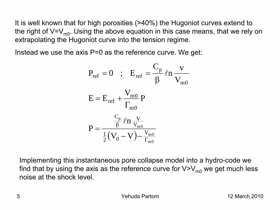
It is well known that for high porosities (>40%) the Hugoniot curves extend to the right of V=Vm0

. Using the above equation in this case means, that we rely on extrapolating the Hugoniot curve into the tension regime.

Instead we use the axis P=0 as the reference curve. We get:

( )0m

0m

0m

p

V02

1

VVC

0m

0mref

0m

prefref

VV

nP

PVEE

Vvn

CE;0P

Γ

β

−−=

Γ+=

β==

l

l

Implementing this instantaneous pore collapse model into a hydro-code we find that by using the axis as the reference curve for V>Vm0

we get much less noise at the shock level.


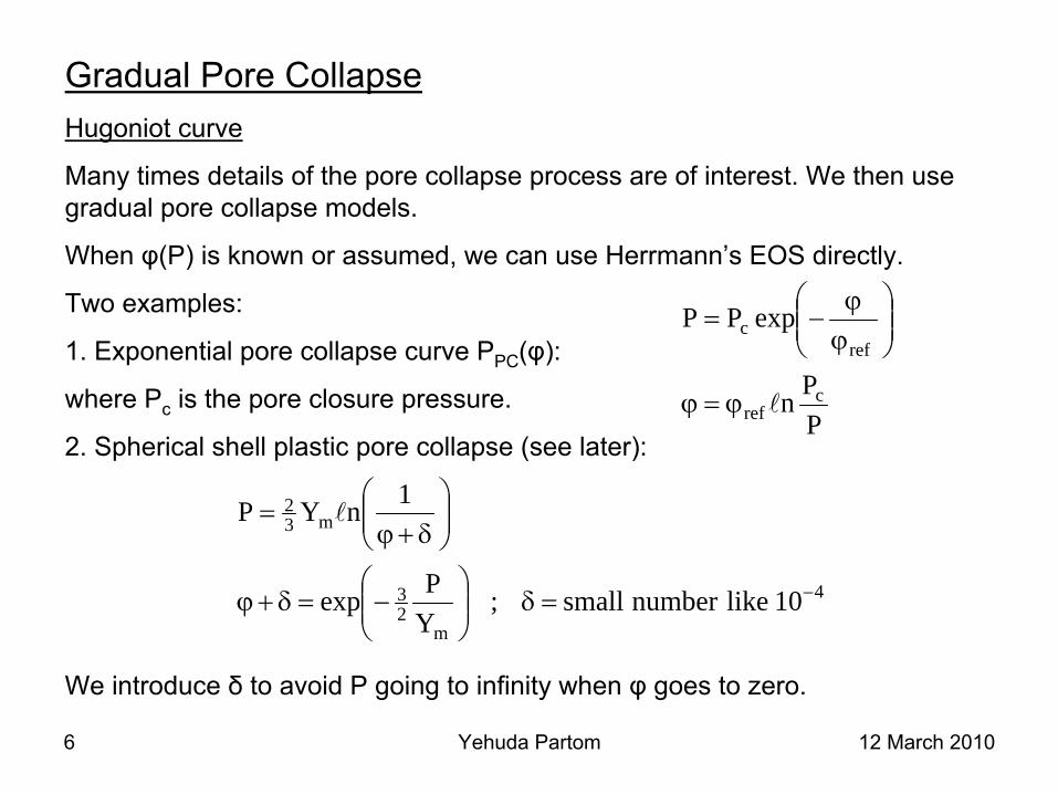
Gradual Pore CollapseHugoniot curve

Many times details of the pore collapse process are of interest.

We then use gradual pore collapse models.

When φ(P) is known or assumed, we can use Herrmann’s EOS directly.

Two examples:

1. Exponential pore collapse curve PPC

(φ):

where Pc

is the pore closure pressure.

2. Spherical shell plastic pore collapse (see later):

We introduce δ

to avoid P going to infinity when φ

goes to zero.

PPn

expPP

cref

refc

lϕ=ϕ

⎟⎟⎠

⎞⎜⎜⎝

⎛ϕϕ

−=

4

m23

m32

10likenumbersmall;YPexp

1nYP

−=δ⎟⎟⎠

⎞⎜⎜⎝

⎛−=δ+ϕ

⎟⎟⎠

⎞⎜⎜⎝

⎛δ+ϕ

= l


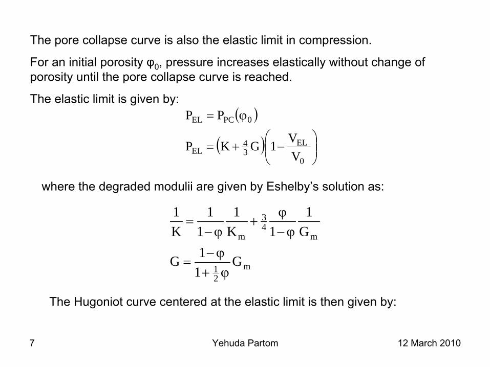
The pore collapse curve is also the elastic limit in compression.

For an initial porosity φ0

, pressure increases elastically without change of porosity until the pore collapse curve is reached.

The elastic limit is given by:( )

( ) ⎟⎟⎠

⎞⎜⎜⎝

⎛−+=

ϕ=

0

EL34

EL

0PCEL

VV1GKP

PP

where the degraded modulii are given by Eshelby’s solution as:

m21

m43

m

G11G

G1

1K1

11

K1

ϕ+ϕ−

=

ϕ−ϕ

+ϕ−

=

The Hugoniot curve centered at the elastic limit is then given by:


( )( )

⎟⎟⎠

⎞⎜⎜⎝

⎛−

ϕ−Γ+=

−++=

Hm0m

0mHm

ELEL21

EL

P1

PVEE

VVPPEE

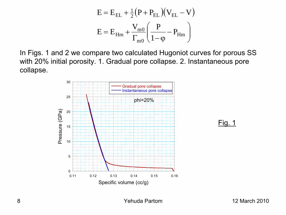
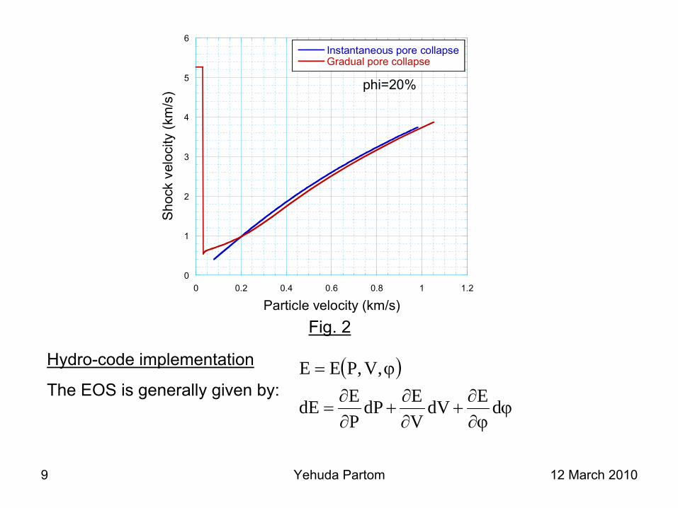
In Figs. 1 and 2 we compare two calculated Hugoniot curves for porous SS with 20% initial porosity. 1. Gradual pore collapse. 2. Instantaneous pore collapse.

Fig. 1

0

5

10

15

20

25

30

0.11 0.12 0.13 0.14 0.15 0.16

Gradual pore collapseInstantaneous pore collapse

Pre

ssur

e (G

Pa)

Specific volume (cc/g)

phi=20%


0

1

2

3

4

5

6

0 0.2 0.4 0.6 0.8 1 1.2

Instantaneous pore collapseGradual pore collapse

Sho

ck v

eloc

ity (k

m/s

)

Particle velocity (km/s)

phi=20%

Fig. 2

Hydro-code implementation

The EOS is generally given by:( )

ϕϕ∂∂

+∂∂

+∂∂

=

ϕ=

dEdVVEdP

PEdE

,V,PEE


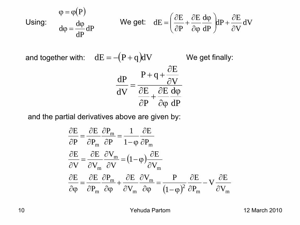
Using:( )

dPdPdd

Pϕ

=ϕ

ϕ=ϕWe get: dV

VEdP

dPdE

PEdE

∂∂

+⎟⎟⎠

⎞⎜⎜⎝

⎛ ϕϕ∂∂

+∂∂

=

and together with: ( )dVqPdE +−= We get finally:

dPdE

PE

VEqP

dVdP

ϕϕ∂∂

+∂∂

∂∂

++=

and the partial derivatives above are given by:

( )

( ) mm2

m

m

m

m

m

m

m

m

m

m

VEV

PE

1PV

VEP

PEE

VE1

VV

VE

VE

PE

11

PP

PE

PE

∂∂

−∂∂

ϕ−=

ϕ∂∂

∂∂

+ϕ∂

∂∂∂

=ϕ∂∂

∂∂

ϕ−=∂∂

∂∂

=∂∂

∂∂

ϕ−=

∂∂

∂∂

=∂∂


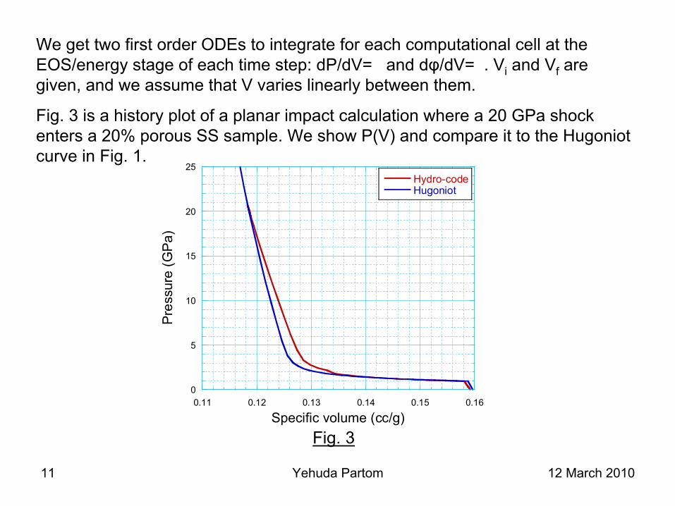
We get two first order ODEs to integrate for each computational cell at the EOS/energy stage of each time step: dP/dV= and dφ/dV= . Vi

and Vf

are given, and we assume that V varies linearly between them.

Fig. 3 is a history plot of a planar impact calculation where a 20 GPa shock enters a 20% porous SS sample. We show P(V) and compare it to the Hugoniot curve in Fig. 1.

0

5

10

15

20

25

0.11 0.12 0.13 0.14 0.15 0.16

Hydro-codeHugoniot

Pre

ssur

e (G

Pa)

Specific volume (cc/g)Fig. 3


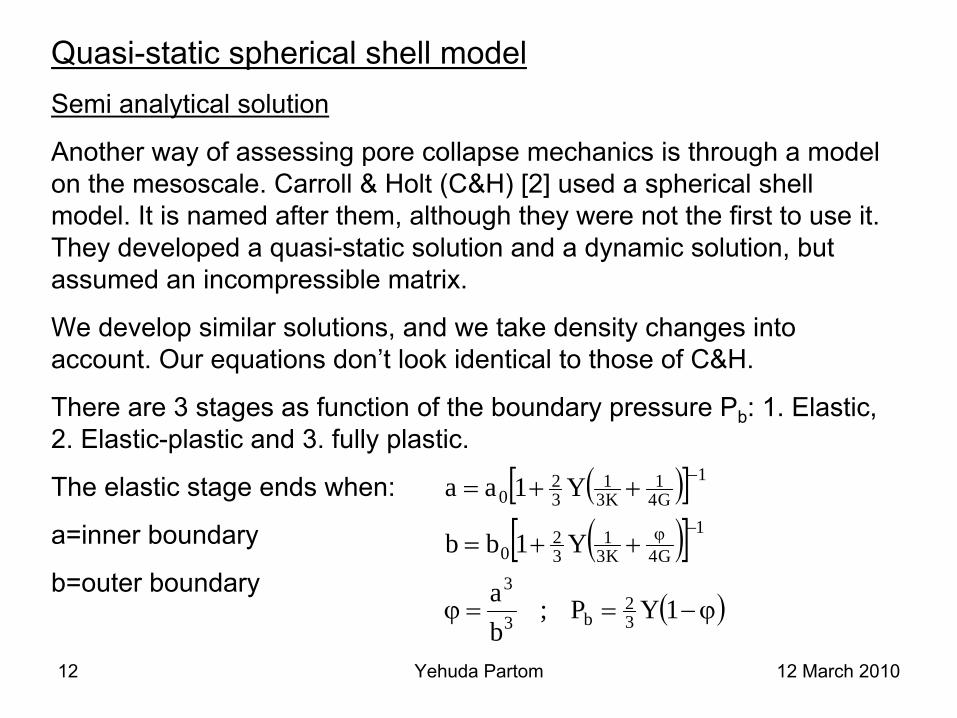
Quasi-static spherical shell modelSemi analytical solution

Another way of assessing pore collapse mechanics is through a model on the mesoscale. Carroll & Holt (C&H) [2] used a spherical shell model. It is named after them, although they were not the first to use it. They developed a quasi-static solution and a dynamic solution, but assumed an incompressible matrix.

We develop similar solutions, and we take density changes into account. Our equations don’t look identical to those of C&H.

There are 3 stages as function of the boundary pressure Pb

: 1. Elastic, 2. Elastic-plastic and 3. fully plastic.

The elastic stage ends when:

a=inner boundary

b=outer boundary

( )[ ]( )[ ]

( )ϕ−==ϕ

++=

++=−ϕ

−

1YP;ba

Y1bb

Y1aa

32

b3

3

1G4K3

132

0

1G41

K31

32

0


At the elastic-plastic stage there are 4 unknowns: a, b, Pb

and the elastic-plastic boundary radius c. If one of them is specified, the others can be determined. It is easiest to specify a. Doing that we get 3 equations with 3 unknowns. The equations express: 1. Equation for b from the elastic field solution. 2. Continuity of σr

across the elastic-plastic boundary. 3. mass conservation. Density changes are included in the third equation by assuming:

The 3 equations are:

To solve these equations we differentiate them with respect to a

and integrate numerically the system of 3 first order ODEs.

⎟⎠⎞

⎜⎝⎛ +ρ=ρ

KP10

( ) 30

30

333

3

32b333

3

3

32

b

2

3

3

3

32

b0

abcbbc

KY

KP1

acnc

KY2ac

bc1YP

acnY2

bc

G6Y

bcYP

K3bbb

−=−⎟⎟⎠

⎞⎜⎜⎝

⎛++++−

⎟⎟⎠

⎞⎜⎜⎝

⎛−−=

−⎟⎟⎠

⎞⎜⎜⎝

⎛+−=

l

l


If and when c reaches the outer boundary (c=b) we enter the fully plastic stage. We have 2 equations: Pb

=σr

(b) and mass conservation:

These can be solved directly by first eliminating .

In Figs. 4 we show results of an example for porous SS with 5 initial porosities φ0

=20%, 10%, 1%, 0.1%, 0.01%. In all the calculations b0

=1mm and a0

has values according to these porosities.

In Figs. 5 we show the Pb

(φ) curves during the pore collapse.

In Fig. 6 we show the Pb

(φ) curve when a becomes less then 0.0001 mm.

We see from the figures that:

•

When φ0

>1%, the elastic-plastic boundary reaches the outer boundary, and most of the collapse is fully plastic.

•

When φ0

<1%,

the elastic plastic boundary approaches the outer boundary, but then turns around and goes back.

30

30

333

b

ababnb

KY2ab

abnY2P

−=+−

=

l

l

abnY2 l


•

When φ0

is very small, the elastic-plastic boundary stays close to the inner boundary, and the pore closure pressure is finite and tends to 2/3Y, as seen from Fig. 6.

0 0.2 0.4 0.6 0.8 1 1.20

100

200

300

400

500

600

700

abc

Radial distance (mm)

Inte

grat

ion

step

num

ber

Phi0=20%

0 0.2 0.4 0.6 0.8 1 1.20

100

200

300

400

500

600

abc


Inte

grat

ion

step

num

ber

phi=10%

0 0.2 0.4 0.6 0.8 1 1.20

500

1000

1500

2000

2500abc


Inte

grat

ion

step

num

ber

phi=1%

0 0.2 0.4 0.6 0.8 1 1.20

200

400

600

800

1000abc


Inte

grat

ion

step

num

ber

phi=.1%

0 0.2 0.4 0.6 0.8 1 1.20

100

200

300

400

500

abc


Inte

grat

ion

step

num

ber

phi=0.01%

Fig. 4


0

1

2

3

4

5

6

0 0.05 0.1 0.15 0.2

Phi=.01%.1%1%10%20%

Pre

ssur

e (G

Pa)

Porosity

0

1

2

3

4

5

6

0 0.002 0.004 0.006 0.008 0.01

Phi=.01%.1%1%10%20%

Pre

ssur

e (G

Pa)

Porosity

Fig. 5

0

0.5

1

1.5

2

2.5

3

3.5

0 0.01 0.02 0.03 0.04 0.05 0.06

Out

side

pre

ssur

e w

hen

a b

ecom

es <

2e-4

mm

(GPa

)

Initial radius of inner boundary (mm)

Fig. 6


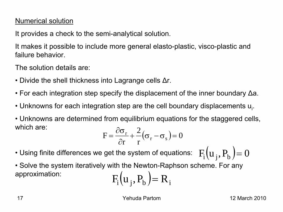
Numerical solution

It provides a check to the semi-analytical solution.

It makes it possible to include more general elasto-plastic, visco-plastic and failure behavior.

The solution details are:

• Divide the shell thickness into Lagrange cells Δr.

• For each integration step specify the displacement of the inner

boundary Δa.

• Unknowns for each integration step are the cell boundary displacements ui

.

•

Unknowns are determined from equilibrium equations for the staggered cells, which are:

• Using finite differences we get the system of equations:

•

Solve the system iteratively with the Newton-Raphson

scheme. For any approximation:

( ) 0r2

rF sr

r =σ−σ+∂σ∂

=

( ) 0P,uF bji =

( ) ibji RP,uF =


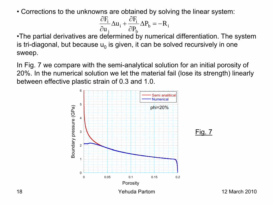
• Corrections to the unknowns are obtained by solving the linear system:

•The partial derivatives are determined by numerical differentiation. The system is tri-diagonal, but because u0

is given, it can be solved recursively in one sweep.

In Fig. 7 we compare with the semi-analytical solution for an initial porosity of 20%. In the numerical solution we let the material fail (lose its strength) linearly between effective plastic strain of 0.3 and 1.0.

ibb

ii

j

i RPPFu

uF

−=Δ∂∂

+Δ∂∂

0

1

2

3

4

5

6

0 0.05 0.1 0.15 0.2

Semi analiticalNumerical

Bou

ndar

y pr

essu

re (G

Pa)

Porosity

phi=20%

Fig. 7


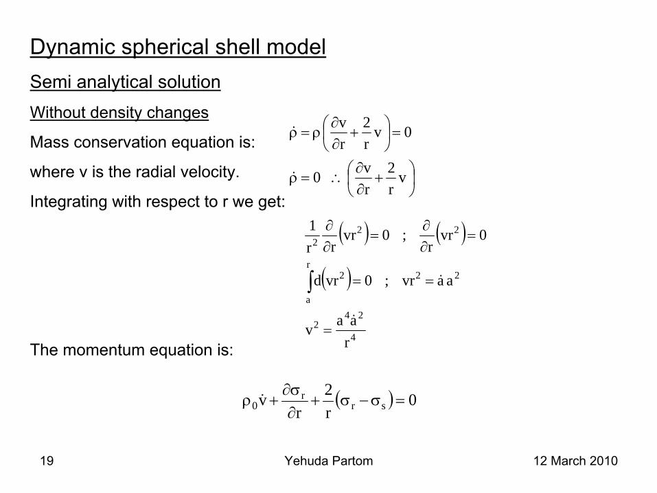
Dynamic spherical shell modelSemi analytical solutionWithout density changes

Mass conservation equation is:

where v is the radial velocity.

Integrating with respect to r we get:

The momentum equation is:

⎟⎠⎞

⎜⎝⎛ +∂∂

∴=ρ

=⎟⎠⎞

⎜⎝⎛ +∂∂

ρ=ρ

vr2

rv0

0vr2

rv

&

&

( ) ( )

( )

4

242

r

a

222

222

raav

aavr;0vrd

0vrr

;0vrrr

1

&

&

=

==

=∂∂

=∂∂

∫

( ) 0r2

rv sr

r0 =σ−σ+

∂σ∂

+ρ &


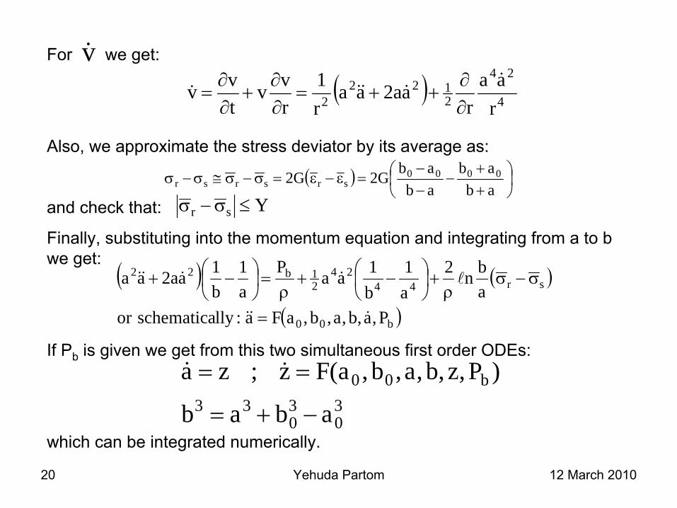
For we get:

Also, we approximate the stress deviator by its average as:

and check that:

Finally, substituting into the momentum equation and integrating

from a to b we get:

If Pb

is given we get from this two simultaneous first order ODEs:

which can be integrated numerically.

v&( ) 4

24

2122

2 raa

raa2aa

r1

rvv

tvv

&&&&&

∂∂

++=∂∂

+∂∂

=

( ) ⎟⎠⎞

⎜⎝⎛

++

−−−

=ε−ε=σ−σ≅σ−σabab

ababG2G2 0000

srsrsr

Ysr ≤σ−σ

( ) ( )

( )b00

sr4424

21b22

P,a,b,a,b,aFa:llyschematicaorabn2

a1

b1aaP

a1

b1aa2aa

&&&

l&&&&

=

σ−σρ

+⎟⎠⎞

⎜⎝⎛ −+

ρ=⎟

⎠⎞

⎜⎝⎛ −+

30

30

33b00

abab

)P,z,b,a,b,a(Fz;za

−+=

== &&


In Fig. 8 we show an example of results using these equations. Again, it is a SS shell with 20% porosity and Pb

=20GPa.

0

0.2

0.4

0.6

0.8

1

1.2

0 0.05 0.1 0.15 0.2 0.25

ab

She

ll ra

dius

(mm

)

Time (microsec)

Phi=20%

Fig. 8

We see from Fig. 8 that towards closure, the inner boundary velocity becomes extremely fast, and will probably get unstable.

We computed closure time as function of Pb

. We show the results in Fig. 9.


Fig. 9

We see from Fig. 9 that for Pb

<1GPa the cavity does not close completely. This is different from the quasi-static solution. Also, we don’t get an elastic-

plastic stage, as we consider only averages of the shear stress components.

Including density changes

Using a similar approach, we’re able to consider average density changes. The mass conservation equation is then:

0

0.5

1

1.5

2

2.5

3

0 5 10 15 20 25

Clo

sure

tim

e (m

icro

sec)

Outer boundary pressure GPa)

phi=20%


ρρ

−=⎟⎠⎞

⎜⎝⎛ +∂∂

=⎟⎠⎞

⎜⎝⎛ +∂∂

ρ+ρ&

& vr2

rv;0v

r2

rv

As before we assume:

sPKsP

KsP

;K

sP1

sPP;KP1

32

b

32

b

32

b

0

32

b

0

32

b0

+++

=ρρ

+=

ρρ+

+=ρρ

+=⎟⎟⎠

⎞⎜⎜⎝

⎛+ρ=ρ

&&&

&&&

The momentum equation is: ( ) 0r2

rv sr

r =σ−σ+∂σ∂

+ρ &

and the over whole mass conservation is:

For a constant Pb

the mass conservation equation is the same as before, and we may proceed as before (ignoring the small influence of the changing of s in the elastic region).

In Fig. 9 we show the porosity history for the same problem as before, and compare it to the result from the constant density run.

( )30

30

033 abab −ρρ

=−


0

0.05

0.1

0.15

0.2

0.25

0 0.05 0.1 0.15 0.2 0.25 0.3

No density changeWith density change

Por

osity

Time (microsec)

Phi=20%

Fig. 9

We see from Fig. 9 that the influence of density change is small, and that it slows the compaction process.

If Pb

=Pb

(t), the system of equations gets extremely complicated. We therefore chose not to work with these equations. Instead we approximate Pb

(t) by a staircase curve so that for each time step we have a constant Pb

. The error introduced can be checked by changing the integration time step.


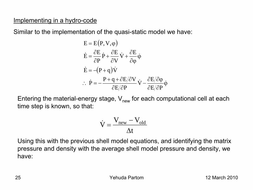
Implementing in a hydro-code

Similar to the implementation of the quasi-static model we have:

( )

( )

ϕ∂∂ϕ∂∂

−∂∂

∂∂++−=∴

+−=

ϕϕ∂∂

+∂∂

+∂∂

=

ϕ=

&&&

&&

&&&&

PEEV

PEVEqPP

VqPE

EVVEP

PEE

,V,PEE

Entering the material-energy stage, Vnew

for each computational cell at each time step is known, so that:

tVVV oldnew

Δ−

=&

Using this with the previous shell model equations, and identifying the matrix pressure and density with the average shell model pressure and density, we have:


( )

( ) ( )

( ) ( )P1P1P;;PPaz13;

ba;abab

P,z,a,,b,aFz;za

mmm

3

330

30

033

b00

ϕ−=ϕ−=ρ=ρ=

ϕ−ϕ=ϕ=ϕ−ρρ

+=

ρ==

&

&&

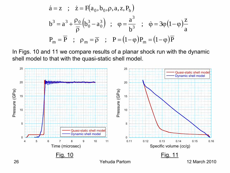
In Figs. 10 and 11 we compare results of a planar shock run with

the dynamic shell model to that with the quasi-static shell model.

0

5

10

15

20

25

4 5 6 7 8 9 10 11

Quasi-static shell modelDynamic shell model

Pre

ssur

e (G

Pa)

Time (microsec)

0

5

10

15

20

25

0.11 0.12 0.13 0.14 0.15 0.16

Quasi-static shell modelDynamic shell model

Pre

ssur

e (G

Pa)


Fig. 10 Fig. 11


We see that there is much difference between the quasi-static and the dynamic models:

•

For the quasi-static model the pores close at a relatively low pressure, while

for the dynamic model they close along the whole pressure range.

• For the dynamic model there is no elastic precursor.

•

For the quasi-static model the shock is sharp, while for the dynamic model the shock is smeared, like for a visco-plastic material.

Dynamic overstress model

For dynamic problems that have an equilibrium or quasi-static solution, the system usually tends towards this solution at a certain rate.

Let the quasi-static solution be:

( )Pqs ϕ=ϕ


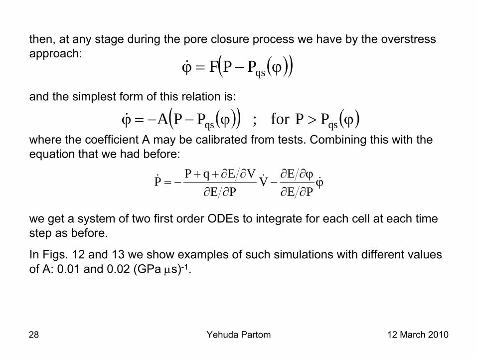
then, at any stage during the pore closure process we have by the overstress approach:

and the simplest form of this relation is:

where the coefficient A may be calibrated from tests. Combining this with the equation that we had before:

we get a system of two first order ODEs to integrate for each cell at each time step as before.

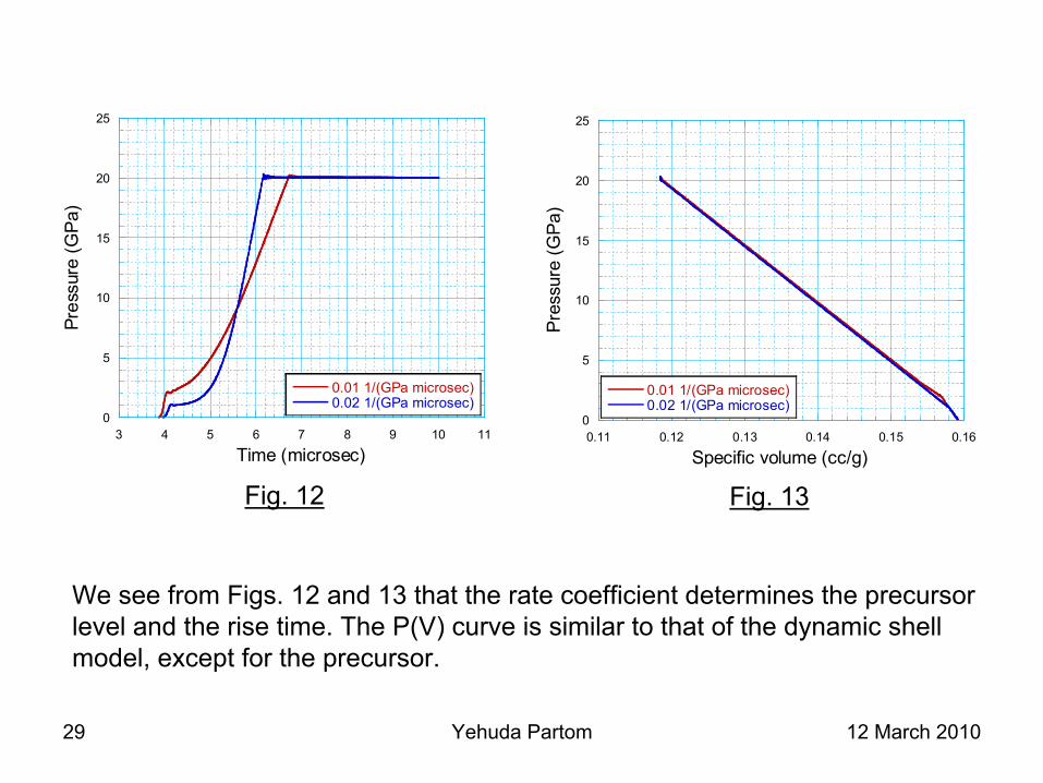
In Figs. 12 and 13 we show examples of such simulations with different values of A: 0.01 and 0.02 (GPa μs)-1.

( )( )ϕ−=ϕ qsPPF&

( )( ) ( )ϕ>ϕ−−=ϕ qsqs PPfor;PPA&

ϕ∂∂ϕ∂∂

−∂∂

∂∂++−= &&&

PEEV

PEVEqPP


0

5

10

15

20

25

3 4 5 6 7 8 9 10 11

0.01 1/(GPa microsec)0.02 1/(GPa microsec)

Pres

sure

(GPa

)

Time (microsec)

0

5

10

15

20

25

0.11 0.12 0.13 0.14 0.15 0.16

0.01 1/(GPa microsec)0.02 1/(GPa microsec)

Pres

sure

(GPa

)


Fig. 12 Fig. 13

We see from Figs. 12 and 13 that the rate coefficient determines

the precursor level and the rise time. The P(V) curve is similar to that of the dynamic shell model, except for the precursor.


SummaryModeling compaction of porous materials started with the pioneering works of Herrmann and Carroll & Holt in the sixties and seventies. Interest in the subject increased when explosive compaction became a viable technology. Never the less, the material models haven’t changed much.

We present a survey of these models. They are based mainly on Herrmann’s EOS and on Carroll & Holts spherical shell model. The examples we show are our own contribution, and the detailed equations are sometimes different from those in the original papers.

The subject is still open to more research because:

• A spherical shell does not represent all possible geometries.

• The models are mainly for ductile materials.

• Collapse under pressure + shear could give different results.

• The size distribution of pores could have an effect.

QUASI-STATIC AND DYNAMIC COMPACTION OF POROUS …

Documents

Transcript of QUASI-STATIC AND DYNAMIC COMPACTION OF POROUS …