PHYSICAL REVIEW B 89, 235102 (2014)

Quantum spin liquid with a Majorana Fermi surfaceon the three-dimensional hyperoctagon lattice

M. Hermanns and S. TrebstInstitute for Theoretical Physics, University of Cologne, 50937 Cologne, Germany

(Received 10 April 2014; revised manuscript received 15 May 2014; published 2 June 2014)

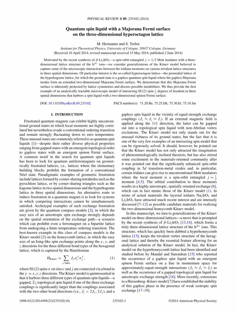
Motivated by the recent synthesis of β-Li2IrO3—a spin-orbit entangled j = 1/2 Mott insulator with a three-dimensional lattice structure of the Ir4+ ions—we consider generalizations of the Kitaev model believed tocapture some of the microscopic interactions between the iridium moments on various trivalent lattice structuresin three spatial dimensions. Of particular interest is the so-called hyperoctagon lattice—the premedial lattice ofthe hyperkagome lattice, for which the ground state is a gapless quantum spin liquid where the gapless Majoranamodes form an extended two-dimensional Majorana Fermi surface. We demonstrate that this Majorana Fermisurface is inherently protected by lattice symmetries and discuss possible instabilities. We thus provide the firstexample of an analytically tractable microscopic model of interacting SU(2) spin- 1

2 degrees of freedom in threespatial dimensions that harbors a spin liquid with a two-dimensional spinon Fermi surface.

DOI: 10.1103/PhysRevB.89.235102 PACS number(s): 71.20.Be, 75.25.Dk, 75.30.Et, 75.10.Jm

I. INTRODUCTION

Frustrated quantum magnets can exhibit highly unconven-tional ground states in which local moments are highly corre-lated but nevertheless evade a conventional ordering transitionand remain strongly fluctuating down to zero temperature.These unusual states are commonly referred to as quantum spinliquids [1]—despite their rather diverse physical propertiesranging from gapped states with an emergent topological orderto gapless states with an emergent spinon Fermi surface.A common motif in the search for quantum spin liquidshas been to look for quantum antiferromagnets on geomet-rically frustrated lattices, i.e., lattices where the elementarybuilding blocks prohibit the formation of a conventionalNeel state. Paradigmatic examples of geometric frustrationinclude lattices formed by corner-sharing tetrahedra such as thepyrochlore lattice, or by corner-sharing triangles such as thekagome lattice in two spatial dimensions and the hyperkagomelattice in three spatial dimensions. An alternative route toinduce frustration in a quantum magnet is to look for systemsin which competing interactions cannot be simultaneouslysatisfied. Archetypal examples of such exchange frustrationare given by the quantum compass models [2], in which theeasy axis of an anisotropic spin exchange strongly dependson the spatial orientation of the exchange path—a scenariowhich can prohibit even a ferromagnet on a bipartite latticefrom undergoing a finite-temperature ordering transition. Thebest-known example in this class of compass models is theKitaev model [3] on the honeycomb lattice, in which the easyaxis of an Ising-like spin exchange points along the x, y, andz directions for the three different bond types of the hexagonallattice, which is captured by the Hamiltonian

HKitaev =∑

γ links

Jγ σγ

i σγ

j , (1)

where SU(2) spins σ on sites i and j are connected via a bond inthe γ = x,y,z directions. The Kitaev model is quintessential inthat it harbors three different types of quantum spin liquids—agapped, Z2 topological spin liquid if one of the three exchangecouplings is significantly larger than the couplings associatedwith the two other bond directions (i.e., Jz > 2Jx, 2Jy), and a

gapless spin liquid in the vicinity of equal-strength exchangecouplings (Jx ≈ Jy ≈ Jz). If an external magnetic field isapplied along the 111 direction, the latter can be gappedout into a topological spin liquid with non-Abelian vortexexcitations. The Kitaev model not only stands out for theunusual richness of its ground states, but the fact that it isone of the very few examples of an interacting spin model thatcan be rigorously solved. It should, however, be pointed outthat the Kitaev model has not only attracted the imaginationof phenomenologically inclined theorists, but has also stirredsome excitement in the materials-oriented community afterit was pointed out that the significantly enhanced spin-orbitcoupling in 5d transition-metal oxides and, in particular,certain iridates can give rise to unconventional Mott insulatorswhere the local moment is a spin-orbit entangled j = 1

2moment [4,5]. The orbital contribution to these momentsresults in a highly anisotropic, spatially oriented exchange [6],which can in fact mimic those of the Kitaev model (1). Interms of actual materials the layered iridates Na2IrO3 andLi2IrO3 have attracted much recent interest and are intenselydiscussed [7–12] as possible candidate materials for realizingthe two-dimensional honeycomb Kitaev model.

In this manuscript, we turn to generalizations of the Kitaevmodel on three-dimensional lattices—a move that is promptedby the recent synthesis of β-Li2IrO3 [13,14], which forms atruly three-dimensional lattice structure of the Ir4+ ions. Thisstructure, which has quickly been dubbed a hyperhoneycomblattice [13], keeps the trivalent vertex structure of the hexag-onal lattice and thereby the essential feature allowing for ananalytical solution of the Kitaev model. In fact, the Kitaevmodel on the hyperhoneycomb lattice had been identified andstudied before by Mandal and Surendran [15] who reportedthe occurrence of a gapless spin liquid with an emergentspinon Fermi surface on a line in momentum space forapproximately-equal-strength interactions (Jx ≈ Jy ≈ Jz) aswell as the occurrence of a gapped topological spin liquid foranisotropic exchange strength [16]. More recently, extensionsto a Heisenberg–Kitaev model [7] have established the stabilityof this gapless phase in the presence of weak isotropic spinexchange [17–19].

1098-0121/2014/89(23)/235102(16) 235102-1 ©2014 American Physical Society

M. HERMANNS AND S. TREBST PHYSICAL REVIEW B 89, 235102 (2014)

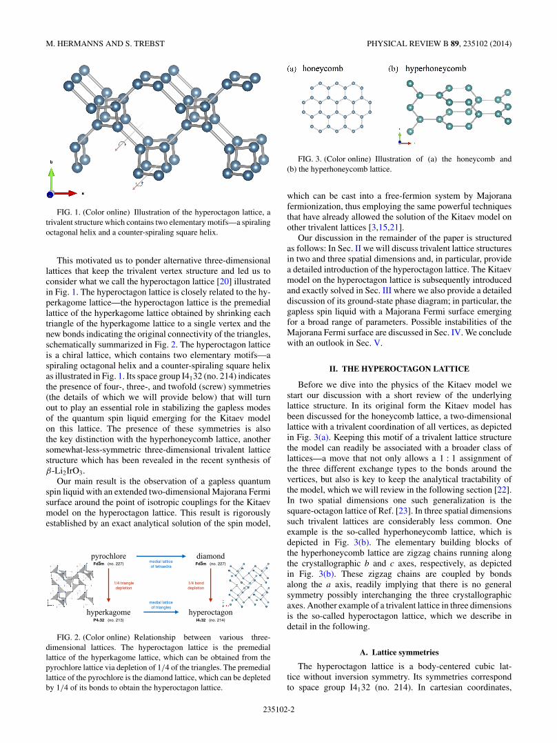
FIG. 1. (Color online) Illustration of the hyperoctagon lattice, atrivalent structure which contains two elementary motifs—a spiralingoctagonal helix and a counter-spiraling square helix.

This motivated us to ponder alternative three-dimensionallattices that keep the trivalent vertex structure and led us toconsider what we call the hyperoctagon lattice [20] illustratedin Fig. 1. The hyperoctagon lattice is closely related to the hy-perkagome lattice—the hyperoctagon lattice is the premediallattice of the hyperkagome lattice obtained by shrinking eachtriangle of the hyperkagome lattice to a single vertex and thenew bonds indicating the original connectivity of the triangles,schematically summarized in Fig. 2. The hyperoctagon latticeis a chiral lattice, which contains two elementary motifs—aspiraling octagonal helix and a counter-spiraling square helixas illustrated in Fig. 1. Its space group I4132 (no. 214) indicatesthe presence of four-, three-, and twofold (screw) symmetries(the details of which we will provide below) that will turnout to play an essential role in stabilizing the gapless modesof the quantum spin liquid emerging for the Kitaev modelon this lattice. The presence of these symmetries is alsothe key distinction with the hyperhoneycomb lattice, anothersomewhat-less-symmetric three-dimensional trivalent latticestructure which has been revealed in the recent synthesis ofβ-Li2IrO3.

Our main result is the observation of a gapless quantumspin liquid with an extended two-dimensional Majorana Fermisurface around the point of isotropic couplings for the Kitaevmodel on the hyperoctagon lattice. This result is rigorouslyestablished by an exact analytical solution of the spin model,

pyrochlore

hyperkagome

diamond

hyperoctagon

medial latticeof tetraedra

medial latticeof triangles

1/4 triangledepletion

1/4 bonddepletion

P4 32 (no. 213) I4 32 (no. 214)

Fd3m (no. 227) Fd3m (no. 227)

FIG. 2. (Color online) Relationship between various three-dimensional lattices. The hyperoctagon lattice is the premediallattice of the hyperkagome lattice, which can be obtained from thepyrochlore lattice via depletion of 1/4 of the triangles. The premediallattice of the pyrochlore is the diamond lattice, which can be depletedby 1/4 of its bonds to obtain the hyperoctagon lattice.

FIG. 3. (Color online) Illustration of (a) the honeycomb and(b) the hyperhoneycomb lattice.

which can be cast into a free-fermion system by Majoranafermionization, thus employing the same powerful techniquesthat have already allowed the solution of the Kitaev model onother trivalent lattices [3,15,21].

Our discussion in the remainder of the paper is structuredas follows: In Sec. II we will discuss trivalent lattice structuresin two and three spatial dimensions and, in particular, providea detailed introduction of the hyperoctagon lattice. The Kitaevmodel on the hyperoctagon lattice is subsequently introducedand exactly solved in Sec. III where we also provide a detaileddiscussion of its ground-state phase diagram; in particular, thegapless spin liquid with a Majorana Fermi surface emergingfor a broad range of parameters. Possible instabilities of theMajorana Fermi surface are discussed in Sec. IV. We concludewith an outlook in Sec. V.

II. THE HYPEROCTAGON LATTICE

Before we dive into the physics of the Kitaev model westart our discussion with a short review of the underlyinglattice structure. In its original form the Kitaev model hasbeen discussed for the honeycomb lattice, a two-dimensionallattice with a trivalent coordination of all vertices, as depictedin Fig. 3(a). Keeping this motif of a trivalent lattice structurethe model can readily be associated with a broader class oflattices—a move that not only allows a 1 : 1 assignment ofthe three different exchange types to the bonds around thevertices, but also is key to keep the analytical tractability ofthe model, which we will review in the following section [22].In two spatial dimensions one such generalization is thesquare-octagon lattice of Ref. [23]. In three spatial dimensionssuch trivalent lattices are considerably less common. Oneexample is the so-called hyperhoneycomb lattice, which isdepicted in Fig. 3(b). The elementary building blocks ofthe hyperhoneycomb lattice are zigzag chains running alongthe crystallographic b and c axes, respectively, as depictedin Fig. 3(b). These zigzag chains are coupled by bondsalong the a axis, readily implying that there is no generalsymmetry possibly interchanging the three crystallographicaxes. Another example of a trivalent lattice in three dimensionsis the so-called hyperoctagon lattice, which we describe indetail in the following.

A. Lattice symmetries

The hyperoctagon lattice is a body-centered cubic lat-tice without inversion symmetry. Its symmetries correspondto space group I4132 (no. 214). In cartesian coordinates,

235102-2

QUANTUM SPIN LIQUID WITH A MAJORANA FERMI . . . PHYSICAL REVIEW B 89, 235102 (2014)

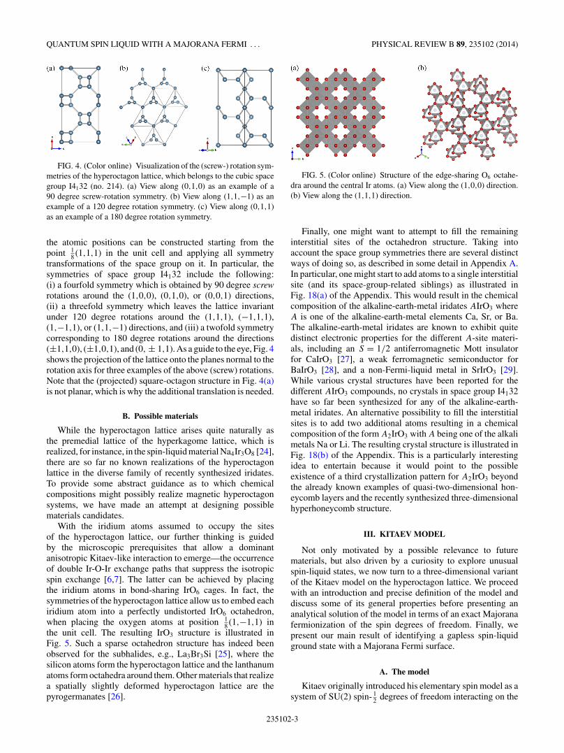
FIG. 4. (Color online) Visualization of the (screw-) rotation sym-metries of the hyperoctagon lattice, which belongs to the cubic spacegroup I4132 (no. 214). (a) View along (0,1,0) as an example of a90 degree screw-rotation symmetry. (b) View along (1,1,−1) as anexample of a 120 degree rotation symmetry. (c) View along (0,1,1)as an example of a 180 degree rotation symmetry.

the atomic positions can be constructed starting from thepoint 1

8 (1,1,1) in the unit cell and applying all symmetrytransformations of the space group on it. In particular, thesymmetries of space group I4132 include the following:(i) a fourfold symmetry which is obtained by 90 degree screwrotations around the (1,0,0), (0,1,0), or (0,0,1) directions,(ii) a threefold symmetry which leaves the lattice invariantunder 120 degree rotations around the (1,1,1), (−1,1,1),(1,−1,1), or (1,1,−1) directions, and (iii) a twofold symmetrycorresponding to 180 degree rotations around the directions(±1,1,0), (±1,0,1), and (0, ± 1,1). As a guide to the eye, Fig. 4shows the projection of the lattice onto the planes normal to therotation axis for three examples of the above (screw) rotations.Note that the (projected) square-octagon structure in Fig. 4(a)is not planar, which is why the additional translation is needed.

B. Possible materials

While the hyperoctagon lattice arises quite naturally asthe premedial lattice of the hyperkagome lattice, which isrealized, for instance, in the spin-liquid material Na4Ir3O8 [24],there are so far no known realizations of the hyperoctagonlattice in the diverse family of recently synthesized iridates.To provide some abstract guidance as to which chemicalcompositions might possibly realize magnetic hyperoctagonsystems, we have made an attempt at designing possiblematerials candidates.

With the iridium atoms assumed to occupy the sitesof the hyperoctagon lattice, our further thinking is guidedby the microscopic prerequisites that allow a dominantanisotropic Kitaev-like interaction to emerge—the occurrenceof double Ir-O-Ir exchange paths that suppress the isotropicspin exchange [6,7]. The latter can be achieved by placingthe iridium atoms in bond-sharing IrO6 cages. In fact, thesymmetries of the hyperoctagon lattice allow us to embed eachiridium atom into a perfectly undistorted IrO6 octahedron,when placing the oxygen atoms at position 1

8 (1,−1,1) inthe unit cell. The resulting IrO3 structure is illustrated inFig. 5. Such a sparse octahedron structure has indeed beenobserved for the subhalides, e.g., La3Br3Si [25], where thesilicon atoms form the hyperoctagon lattice and the lanthanumatoms form octahedra around them. Other materials that realizea spatially slightly deformed hyperoctagon lattice are thepyrogermanates [26].

FIG. 5. (Color online) Structure of the edge-sharing O6 octahe-dra around the central Ir atoms. (a) View along the (1,0,0) direction.(b) View along the (1,1,1) direction.

Finally, one might want to attempt to fill the remaininginterstitial sites of the octahedron structure. Taking intoaccount the space group symmetries there are several distinctways of doing so, as described in some detail in Appendix A.In particular, one might start to add atoms to a single interstitialsite (and its space-group-related siblings) as illustrated inFig. 18(a) of the Appendix. This would result in the chemicalcomposition of the alkaline-earth-metal iridates AIrO3 whereA is one of the alkaline-earth-metal elements Ca, Sr, or Ba.The alkaline-earth-metal iridates are known to exhibit quitedistinct electronic properties for the different A-site materi-als, including an S = 1/2 antiferromagnetic Mott insulatorfor CaIrO3 [27], a weak ferromagnetic semiconductor forBaIrO3 [28], and a non-Fermi-liquid metal in SrIrO3 [29].While various crystal structures have been reported for thedifferent AIrO3 compounds, no crystals in space group I4132have so far been synthesized for any of the alkaline-earth-metal iridates. An alternative possibility to fill the interstitialsites is to add two additional atoms resulting in a chemicalcomposition of the form A2IrO3 with A being one of the alkalimetals Na or Li. The resulting crystal structure is illustrated inFig. 18(b) of the Appendix. This is a particularly interestingidea to entertain because it would point to the possibleexistence of a third crystallization pattern for A2IrO3 beyondthe already known examples of quasi-two-dimensional hon-eycomb layers and the recently synthesized three-dimensionalhyperhoneycomb structure.

III. KITAEV MODEL

Not only motivated by a possible relevance to futurematerials, but also driven by a curiosity to explore unusualspin-liquid states, we now turn to a three-dimensional variantof the Kitaev model on the hyperoctagon lattice. We proceedwith an introduction and precise definition of the model anddiscuss some of its general properties before presenting ananalytical solution of the model in terms of an exact Majoranafermionization of the spin degrees of freedom. Finally, wepresent our main result of identifying a gapless spin-liquidground state with a Majorana Fermi surface.

A. The model

Kitaev originally introduced his elementary spin model as asystem of SU(2) spin- 1

2 degrees of freedom interacting on the

235102-3

M. HERMANNS AND S. TREBST PHYSICAL REVIEW B 89, 235102 (2014)

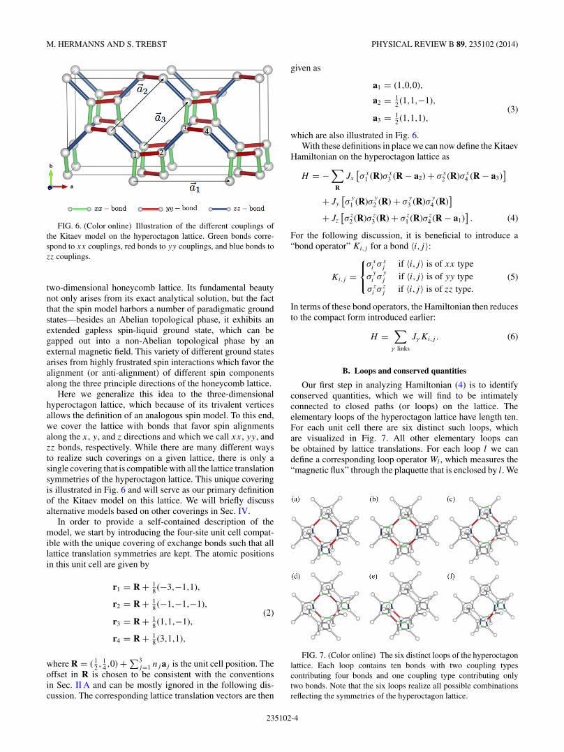
FIG. 6. (Color online) Illustration of the different couplings ofthe Kitaev model on the hyperoctagon lattice. Green bonds corre-spond to xx couplings, red bonds to yy couplings, and blue bonds tozz couplings.

two-dimensional honeycomb lattice. Its fundamental beautynot only arises from its exact analytical solution, but the factthat the spin model harbors a number of paradigmatic groundstates—besides an Abelian topological phase, it exhibits anextended gapless spin-liquid ground state, which can begapped out into a non-Abelian topological phase by anexternal magnetic field. This variety of different ground statesarises from highly frustrated spin interactions which favor thealignment (or anti-alignment) of different spin componentsalong the three principle directions of the honeycomb lattice.

Here we generalize this idea to the three-dimensionalhyperoctagon lattice, which because of its trivalent verticesallows the definition of an analogous spin model. To this end,we cover the lattice with bonds that favor spin alignmentsalong the x, y, and z directions and which we call xx, yy, andzz bonds, respectively. While there are many different waysto realize such coverings on a given lattice, there is only asingle covering that is compatible with all the lattice translationsymmetries of the hyperoctagon lattice. This unique coveringis illustrated in Fig. 6 and will serve as our primary definitionof the Kitaev model on this lattice. We will briefly discussalternative models based on other coverings in Sec. IV.

In order to provide a self-contained description of themodel, we start by introducing the four-site unit cell compat-ible with the unique covering of exchange bonds such that alllattice translation symmetries are kept. The atomic positionsin this unit cell are given by

r1 = R + 18 (−3,−1,1),

r2 = R + 18 (−1,−1,−1),

(2)r3 = R + 1

8 (1,1,−1),

r4 = R + 18 (3,1,1),

where R = ( 12 , 1

4 ,0) + ∑3j=1 nj aj is the unit cell position. The

offset in R is chosen to be consistent with the conventionsin Sec. II A and can be mostly ignored in the following dis-cussion. The corresponding lattice translation vectors are then

given as

a1 = (1,0,0),

a2 = 12 (1,1,−1),

(3)a3 = 1

2 (1,1,1),

which are also illustrated in Fig. 6.With these definitions in place we can now define the Kitaev

Hamiltonian on the hyperoctagon lattice as

H = −∑

R

Jx

[σx

1 (R)σx3 (R − a2) + σx

2 (R)σx4 (R − a3)

]+ Jy

[σ

y

1 (R)σy

2 (R) + σy

3 (R)σy

4 (R)]

+ Jz

[σ z

2 (R)σ z3 (R) + σ z

1 (R)σ z4 (R − a1)

]. (4)

For the following discussion, it is beneficial to introduce a“bond operator” Ki,j for a bond 〈i,j 〉:

Ki,j =⎧⎨⎩

σxi σ x

j if 〈i,j 〉 is of xx typeσ

y

i σy

j if 〈i,j 〉 is of yy typeσ z

i σ zj if 〈i,j 〉 is of zz type.

(5)

In terms of these bond operators, the Hamiltonian then reducesto the compact form introduced earlier:

H =∑

γ links

Jγ Ki,j . (6)

B. Loops and conserved quantities

Our first step in analyzing Hamiltonian (4) is to identifyconserved quantities, which we will find to be intimatelyconnected to closed paths (or loops) on the lattice. Theelementary loops of the hyperoctagon lattice have length ten.For each unit cell there are six distinct such loops, whichare visualized in Fig. 7. All other elementary loops canbe obtained by lattice translations. For each loop l we candefine a corresponding loop operator Wl , which measures the“magnetic flux” through the plaquette that is enclosed by l. We

FIG. 7. (Color online) The six distinct loops of the hyperoctagonlattice. Each loop contains ten bonds with two coupling typescontributing four bonds and one coupling type contributing onlytwo bonds. Note that the six loops realize all possible combinationsreflecting the symmetries of the hyperoctagon lattice.

235102-4

QUANTUM SPIN LIQUID WITH A MAJORANA FERMI . . . PHYSICAL REVIEW B 89, 235102 (2014)

can define the loop operator by the product of bond operatorsof all the bonds contained in the loop

Wl =∏〈i,j〉

Ki,j . (7)

Because of the even length of the loops, these loop operatorssquare to the identity, thus they have eigenvalues ±1. It canfurther be verified that the loop operators commute withHamiltonian (4) as well as with each other. Each loop operatorthus defines an “integral of motion” and a correspondingconserved quantity—the extensive number of which greatlysimplifies the problem. For one, we can divide the Hilbert spaceinto distinct sectors that are each labeled by the eigenvaluesof all the loop operators Wl and restrict the Hamiltonian to aparticular sector.

Before proceeding we note that an alternative definition ofthe loop operators can be formulated as a product over all sitescontained in the loop:

Wl =∏i∈l

σγi

i , (8)

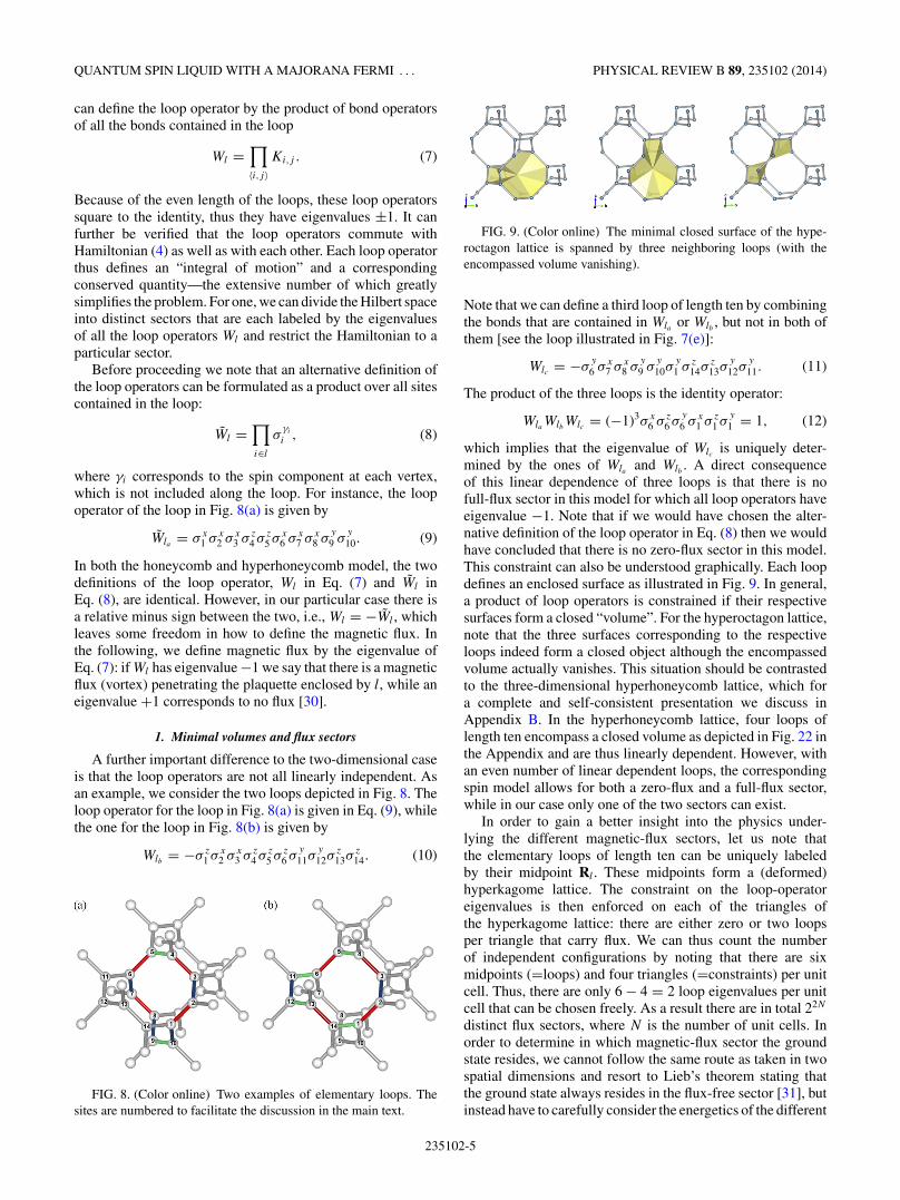
where γi corresponds to the spin component at each vertex,which is not included along the loop. For instance, the loopoperator of the loop in Fig. 8(a) is given by

Wla = σx1 σx

2 σx3 σ z

4 σ z5 σx

6 σx7 σx

8 σy

9 σy

10. (9)

In both the honeycomb and hyperhoneycomb model, the twodefinitions of the loop operator, Wl in Eq. (7) and Wl inEq. (8), are identical. However, in our particular case there isa relative minus sign between the two, i.e., Wl = −Wl , whichleaves some freedom in how to define the magnetic flux. Inthe following, we define magnetic flux by the eigenvalue ofEq. (7): if Wl has eigenvalue −1 we say that there is a magneticflux (vortex) penetrating the plaquette enclosed by l, while aneigenvalue +1 corresponds to no flux [30].

1. Minimal volumes and flux sectors

A further important difference to the two-dimensional caseis that the loop operators are not all linearly independent. Asan example, we consider the two loops depicted in Fig. 8. Theloop operator for the loop in Fig. 8(a) is given in Eq. (9), whilethe one for the loop in Fig. 8(b) is given by

Wlb = −σ z1 σx

2 σx3 σ z

4 σ z5 σ z

6 σy

11σy

12σz13σ

z14. (10)

FIG. 8. (Color online) Two examples of elementary loops. Thesites are numbered to facilitate the discussion in the main text.

FIG. 9. (Color online) The minimal closed surface of the hype-roctagon lattice is spanned by three neighboring loops (with theencompassed volume vanishing).

Note that we can define a third loop of length ten by combiningthe bonds that are contained in Wla or Wlb , but not in both ofthem [see the loop illustrated in Fig. 7(e)]:

Wlc = −σy

6 σx7 σx

8 σy

9 σy

10σy

1 σ z14σ

z13σ

y

12σy

11. (11)

The product of the three loops is the identity operator:

WlaWlbWlc = (−1)3σx6 σ z

6 σy

6 σx1 σ z

1 σy

1 = 1, (12)

which implies that the eigenvalue of Wlc is uniquely deter-mined by the ones of Wla and Wlb . A direct consequenceof this linear dependence of three loops is that there is nofull-flux sector in this model for which all loop operators haveeigenvalue −1. Note that if we would have chosen the alter-native definition of the loop operator in Eq. (8) then we wouldhave concluded that there is no zero-flux sector in this model.This constraint can also be understood graphically. Each loopdefines an enclosed surface as illustrated in Fig. 9. In general,a product of loop operators is constrained if their respectivesurfaces form a closed “volume”. For the hyperoctagon lattice,note that the three surfaces corresponding to the respectiveloops indeed form a closed object although the encompassedvolume actually vanishes. This situation should be contrastedto the three-dimensional hyperhoneycomb lattice, which fora complete and self-consistent presentation we discuss inAppendix B. In the hyperhoneycomb lattice, four loops oflength ten encompass a closed volume as depicted in Fig. 22 inthe Appendix and are thus linearly dependent. However, withan even number of linear dependent loops, the correspondingspin model allows for both a zero-flux and a full-flux sector,while in our case only one of the two sectors can exist.

In order to gain a better insight into the physics under-lying the different magnetic-flux sectors, let us note thatthe elementary loops of length ten can be uniquely labeledby their midpoint Rl . These midpoints form a (deformed)hyperkagome lattice. The constraint on the loop-operatoreigenvalues is then enforced on each of the triangles ofthe hyperkagome lattice: there are either zero or two loopsper triangle that carry flux. We can thus count the numberof independent configurations by noting that there are sixmidpoints (=loops) and four triangles (=constraints) per unitcell. Thus, there are only 6 − 4 = 2 loop eigenvalues per unitcell that can be chosen freely. As a result there are in total 22N

distinct flux sectors, where N is the number of unit cells. Inorder to determine in which magnetic-flux sector the groundstate resides, we cannot follow the same route as taken in twospatial dimensions and resort to Lieb’s theorem stating thatthe ground state always resides in the flux-free sector [31], butinstead have to carefully consider the energetics of the different

235102-5

M. HERMANNS AND S. TREBST PHYSICAL REVIEW B 89, 235102 (2014)

flux sectors. For the great majority of points in parameterspace, we numerically observe that creating or enlarging loopscosts energy and as such the ground state lies in the flux-freesector also in three spatial dimensions. We therefore restrictour following discussion to the zero-flux sector.

Let us briefly consider the effective theory for the magnetic-flux excitations arising from flipping a loop operator eigen-value from +1 to −1. We note that the midpoints of loopswith loop operator eigenvalue −1 form themselves closed loopconfigurations, which live again on the links of a hyperoctagonlattice—albeit with opposite chirality to the original one. Dueto the constraint, only closed-loop configurations are allowed,i.e., there are no magnetic monopoles in this Z2 theory.

C. Majorana representation

We now proceed to discuss the exact analytic solution ofHamiltonian (4). In analogy to the two-dimensional Kitaevmodel, such an analytical solution is possible by recastingthe original spin degrees of freedom in terms of Majoranafermions—a step that effectively reduces the interacting spinsystem to a free-fermion problem, which is given by Majoranafermions hopping in a static gauge field [32]. The fermionsystem can thus be diagonalized in a straightforward way,thereby also revealing the physics of the interacting-spinmodel.

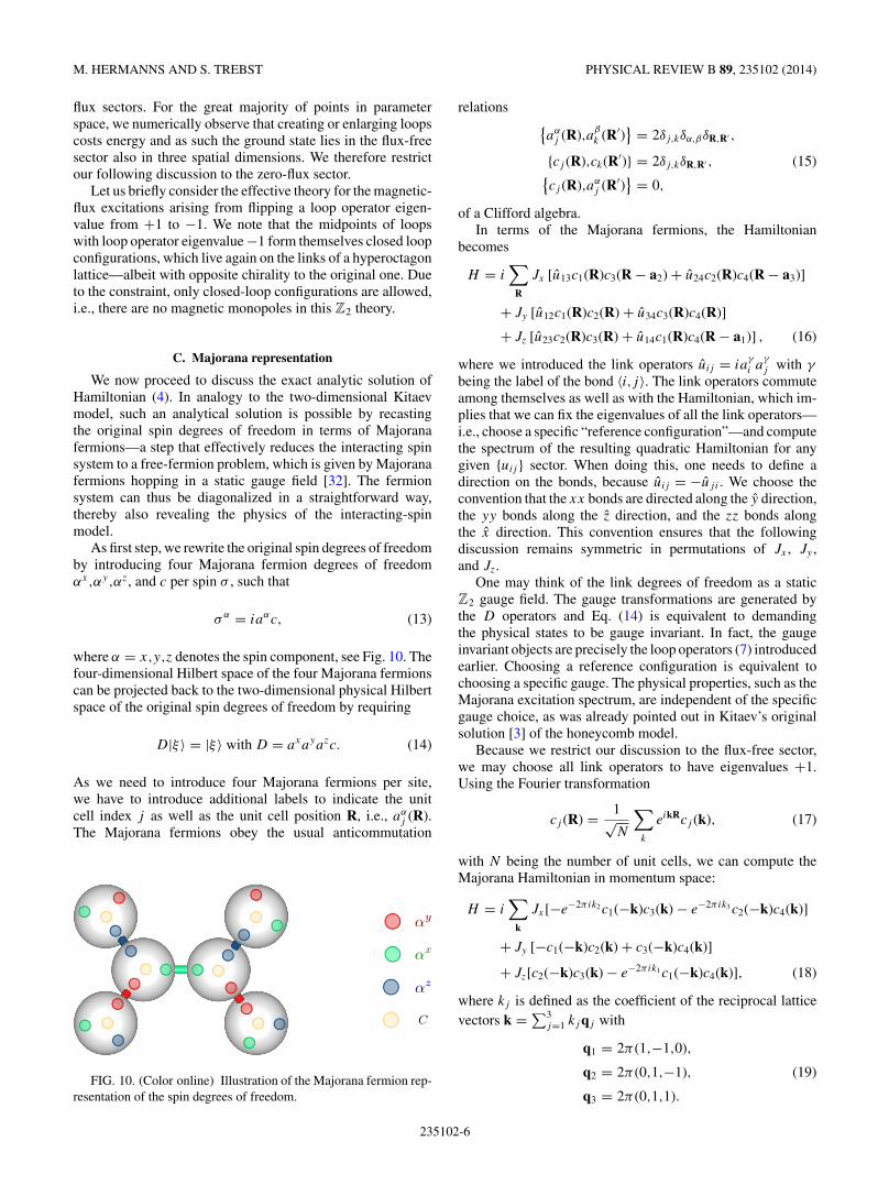
As first step, we rewrite the original spin degrees of freedomby introducing four Majorana fermion degrees of freedomαx,αy,αz, and c per spin σ , such that

σα = iaαc, (13)

where α = x,y,z denotes the spin component, see Fig. 10. Thefour-dimensional Hilbert space of the four Majorana fermionscan be projected back to the two-dimensional physical Hilbertspace of the original spin degrees of freedom by requiring

D|ξ 〉 = |ξ 〉 with D = axayazc. (14)

As we need to introduce four Majorana fermions per site,we have to introduce additional labels to indicate the unitcell index j as well as the unit cell position R, i.e., aα

j (R).The Majorana fermions obey the usual anticommutation

C

αx

αy

αz

FIG. 10. (Color online) Illustration of the Majorana fermion rep-resentation of the spin degrees of freedom.

relations {aα

j (R),aβ

k (R′)} = 2δj,kδα,βδR,R′ ,

{cj (R),ck(R′)} = 2δj,kδR,R′ , (15){cj (R),aα

j (R′)} = 0,

of a Clifford algebra.In terms of the Majorana fermions, the Hamiltonian

becomes

H = i∑

R

Jx [u13c1(R)c3(R − a2) + u24c2(R)c4(R − a3)]

+ Jy [u12c1(R)c2(R) + u34c3(R)c4(R)]

+ Jz [u23c2(R)c3(R) + u14c1(R)c4(R − a1)] , (16)

where we introduced the link operators uij = iaγ

i aγ

j with γ

being the label of the bond 〈i,j 〉. The link operators commuteamong themselves as well as with the Hamiltonian, which im-plies that we can fix the eigenvalues of all the link operators—i.e., choose a specific “reference configuration”—and computethe spectrum of the resulting quadratic Hamiltonian for anygiven {uij } sector. When doing this, one needs to define adirection on the bonds, because uij = −uj i . We choose theconvention that the xx bonds are directed along the y direction,the yy bonds along the z direction, and the zz bonds alongthe x direction. This convention ensures that the followingdiscussion remains symmetric in permutations of Jx , Jy ,and Jz.

One may think of the link degrees of freedom as a staticZ2 gauge field. The gauge transformations are generated bythe D operators and Eq. (14) is equivalent to demandingthe physical states to be gauge invariant. In fact, the gaugeinvariant objects are precisely the loop operators (7) introducedearlier. Choosing a reference configuration is equivalent tochoosing a specific gauge. The physical properties, such as theMajorana excitation spectrum, are independent of the specificgauge choice, as was already pointed out in Kitaev’s originalsolution [3] of the honeycomb model.

Because we restrict our discussion to the flux-free sector,we may choose all link operators to have eigenvalues +1.Using the Fourier transformation

cj (R) = 1√N

∑k

eikRcj (k), (17)

with N being the number of unit cells, we can compute theMajorana Hamiltonian in momentum space:

H = i∑

k

Jx[−e−2πik2c1(−k)c3(k) − e−2πik3c2(−k)c4(k)]

+ Jy [−c1(−k)c2(k) + c3(−k)c4(k)]

+ Jz[c2(−k)c3(k) − e−2πik1c1(−k)c4(k)], (18)

where kj is defined as the coefficient of the reciprocal latticevectors k = ∑3

j=1 kj qj with

q1 = 2π (1,−1,0),

q2 = 2π (0,1,−1), (19)

q3 = 2π (0,1,1).

235102-6

QUANTUM SPIN LIQUID WITH A MAJORANA FERMI . . . PHYSICAL REVIEW B 89, 235102 (2014)

Arriving at Hamiltonian (18) has thus reduced the originalproblem to a four-band Hamiltonian that can be easilydiagonalized [3].

D. Phase diagram

From the diagonal form of the Hamiltonian (18) we canreadily read off the elementary structure of the phase diagramin (Jx,Jy,Jz)-parameter space by carefully analyzing theexcitation spectrum of the Majorana sector. In particular, weobserve that the Hamiltonian allows for zero-energy solutionsindicative of a gapless phase in a range of parameters, whileboth the excitations of the Majorana sector and the magnetic-flux sector remain gapped in other parts of the phase diagram.

The occurrence of zero-energy solutions is equivalent torequiring that det H (k) = 0, which becomes

det[H (k)] = 116

[J 4

x + J 4y + J 4

z + 2J 2y J 2

z cos(kx)

+ 2J 2x J 2

z cos(ky) + 2J 2x J 2

y cos(kz)] ≡ 0 (20)

in cartesian coordinates. In order to determine whether or notthe above equation has solutions, let us analyze the limitingbehavior of the determinant. Expression (20) is bounded fromabove by

det[H (k)] � 116

(J 2

x + J 2y + J 2

z

)2, (21)

when setting cos(kx) = cos(ky) = cos(kz) = 1 and boundedfrom below by

det[H (k)] � − 116 (Jx + Jy − Jz)(Jx + Jz − Jy)

× (Jy + Jz − Jx)(Jx + Jy + Jz), (22)

when setting cos(kx) = cos(ky) = cos(kz) = −1. As the upperbound is always strictly positive, there is a zero-energy solutionif and only if the lower bound is negative (or zero). The latteris equivalent to requiring the triangular inequality

|Jx | + |Jy | � |Jz|,|Jx | + |Jz| � |Jy |, (23)

|Jy | + |Jz| � |Jx |.This is straightforward to derive from Eq. (22) in case allcoupling constants are positive. For the case that at least oneof the coupling constants is negative, we note that Eq. (20)depends only on the squares of the coupling constants. As aconsequence, the upper and lower bounds are independent ofthe signs of the coupling constants.

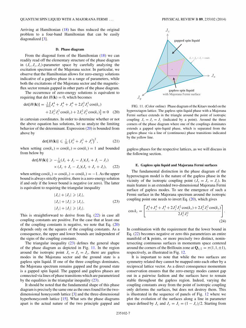
The triangular inequality (23) defines the general shapeof the phase diagram as depicted in Fig. 11. In the regionaround the isotropic point Jx = Jy = Jz, there are gaplessmodes in the Majorana sector and the ground state is agapless spin liquid. If one of the three couplings dominates,the Majorana spectrum remains gapped and the ground stateis a gapped spin liquid. The gapped and gapless phases areconnected via lines of phase transitions which are parametrizedby the equalities in the triangular inequality (23).

It should be noted that the fundamental shape of this phasediagram is precisely the same one as the ones found for the two-dimensional honeycomb lattice [3] and the three-dimensionalhyperhoneycomb lattice [15]. What sets the phase diagramsapart is the actual nature of the two principle gapped and

Jz

Jx

Jy

gapped spin liquid

gapless spin liquidwith Majorana Fermi surface

J + J + J = const.

FIG. 11. (Color online) Phase diagram of the Kitaev model on thehyperoctagon lattice. The gapless spin-liquid phase with a MajoranaFermi surface extends in the triangle around the point of isotropiccoupling Jx = Jy = Jz (indicated by a point). Around the threecorners of the phase diagram where one of the couplings dominatesextends a gapped spin-liquid phase, which is separated from thegapless phase via a line of (continuous) phase transitions indicatedby the yellow line.

gapless phases for the respective lattices, as we will discuss inthe following section.

E. Gapless spin liquid and Majorana Fermi surfaces

The fundamental distinction in the phase diagram of thehyperoctagon model is the nature of the gapless phase in thevicinity of the isotropic coupling point (Jx = Jy = Jz). Itsmain feature is an extended two-dimensional Majorana Fermisurface of gapless modes. To see the emergence of such aFermi surface in the Majorana spectrum around the isotropiccoupling point one needs to invert Eq. (20), which gives

cos kz =[J 4

x +J 4y + J 4

z + 2J 2y J 2

z cos(kx) + 2J 2x J 2

z cos(ky)

2J 2x J 2

y

].

(24)

In combination with the requirement that the lower bound inEq. (22) becomes negative or zero this parametrizes an entiremanifold of k points, or more precisely two distinct, nonin-tersecting continuous surfaces in momentum space centeredaround the corners of the Brillouin zone at Q1/2 = π (1,1,±1),respectively, as illustrated in Fig. 12.

It is important to note that while the two surfaces aresymmetry related they cannot be mapped onto each other by areciprocal lattice vector. As a direct consequence momentumconservation ensures that the zero-energy modes cannot gapout in a pairwise fashion and the surfaces have to remainstable throughout the gapless region. Indeed, varying thecoupling constants away from the point of isotropic couplingonly deforms the surfaces, but does not destroy them. Thisis illustrated in the sequence of panels of Fig. 12 where weplot the evolution of the surfaces along a line in parameterspace defined by Jx and Jy = Jz = (1 − Jx)/2. Starting from

235102-7

M. HERMANNS AND S. TREBST PHYSICAL REVIEW B 89, 235102 (2014)

FIG. 12. (Color online) Evolution of the Majorana Fermi surface with varying coupling parameters Jx and Jy = Jz = (1 − Jx)/2. As thephase transition to the gapped spin liquid is approached with increasing Jz (upper row) the Majorana Fermi surface shrinks to a single point atmomenta Q1 = (π,π,π ) and Q2 = (π,π,−π ). Approaching the decoupling point for Jx → 0 (lower row) the Majorana Fermi surface flattensto two planes.

the isotropic point and increasing Jx elongates the surfacealong the x direction and contracts it in the orthogonal y andz directions, as illustrated in the upper panel of Fig. 12. Uponfurther increasing Jx the surface contracts towards the cornerof the Brillouin zone. As one approaches the phase transition tothe gapped spin liquid at Jx = 1/2, the surfaces have reducedto the points Q1/2 at the corners of the Brillouin zone. On theother hand, decreasing Jx from the isotropic point flattens thesurface in the x direction, as illustrated in the lower panel ofFig. 12. As Jx goes to zero the two opposite sides of the surfaceapproach each other and touch precisely at the decouplingpoint Jx = 0 (and at which the notion of a two-dimensionalsurface ultimately breaks down as well).

To reveal the nature of the zero-energy gapless modes weplot the dispersion of the four principal bands of Hamilto-nian (18) along certain high-symmetry lines in Fig. 13. Forthe entire gapless phase the dispersion of the bands crossingzero energy is always linear along the direction normal tothe surface—reminiscent of the energy spectrum of a Fermi

liquid in the vicinity of the Fermi energy. One should, however,keep in mind that the four bands in our Hamiltonian are notspanned by conventional fermionic degrees of freedom, but byMajorana fermions. As such the zero-energy surfaces revealingthemselves in the energy spectrum should in fact be thoughtof as Majorana Fermi surfaces.

As the phase transition to the gapped phase at Jx = 1/2 isapproached, the relevant Majorana band moves up in energyand at Jx = 1/2 no longer crosses the zero-energy level butmerely touches E = 0 in a single point with a quadraticdispersion. This scenario is in complete analogy to the phasetransitions from the gapless to gapped Majorana phases in boththe honeycomb and hyperhoneycomb models.

IV. INSTABILITIES OF MAJORANA FERMI SURFACE

For conventional Fermi liquids it is well appreciated thatthe Fermi surface is susceptible to a variety of instabilities, themost notable of which is the formation of superconductivity.

HΓ

N

P

(a) (b) (c)

Γ P N H Γ N P Hmomentum K

-0.8

-0.4

0

0.4

0.8

ener

gy E(K)

J = 0J = 0.1J = 0.17J = 0.26J = 1/3

Γ P N H Γ N P Hmomentum K

-0.8

-0.4

0

0.4

0.8

ener

gy E(K)

J = 1/2J = 0.46J = 0.42J = 0.37J = 1/3

FIG. 13. (Color online) Band structure of the four principal bands of the Kitaev model along a path connecting the high-symmetry points = (0,0,0), P = (π,π,π ), N = (π,π,0), and H = (0,2π,0) of the Brillouin zone depicted on the left. The dispersion of the elementaryexcitations at the Fermi energy is linear for all couplings 0 < Jx < 1/2 and corresponding couplings Jy = Jz = (1 − Jx)/2. At the transitionto the gapped spin liquid, Jx = 1/2, the dispersion becomes quadratic. At the point Jx = 0 the Hamiltonian reduces to decoupled Jy-Jz spirals,resulting in a flat spectrum between the high-symmetry points P and N .

235102-8

QUANTUM SPIN LIQUID WITH A MAJORANA FERMI . . . PHYSICAL REVIEW B 89, 235102 (2014)

As such two questions immediately arise with regard to theMajorana Fermi surface in our hyperoctagon model—why isthe Majorana Fermi surface stable in the first place and whatare its possible instabilities?

We will address the first question—the stability of theMajorana Fermi surface—in the following by showing thatit can be tracked to the underlying lattice symmetries. We willthen devote the remainder of this section to a discussion ofpossible instabilities of the Majorana Fermi surface focusingon instabilities arising from a reduction in lattice symmetries.

A. Stability of gapless modes

To discuss the stability of the Majorana Fermi surface letus first recall some basic facts about Majorana fermions. Animmediate consequence of the Majorana condition c

†j (R) =

cj (R) in real space is that the “creation operator” c†j (k) in

momentum space is defined by c†j (k) = cj (−k). The latter

implies that for every energy state E(k) there is a “particle-hole-conjugate” partner at −k for which

E(−k) = −E(k).

For clarity, we will suppress the unit cell index in this sectionto make the expressions more accessible. However, one shouldnote that the energy relations generically relate different bandsto each other.

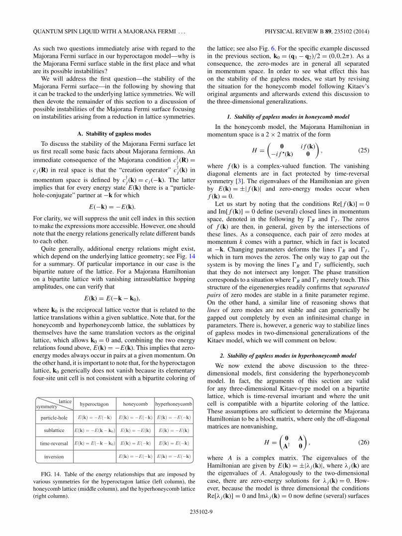
Quite generally, additional energy relations might exist,which depend on the underlying lattice geometry; see Fig. 14for a summary. Of particular importance in our case is thebipartite nature of the lattice. For a Majorana Hamiltonianon a bipartite lattice with vanishing intrasublattice hoppingamplitudes, one can verify that

E(k) = E(−k − k0),

where k0 is the reciprocal lattice vector that is related to thelattice translations within a given sublattice. Note that, for thehoneycomb and hyperhoneycomb lattice, the sublattices bythemselves have the same translation vectors as the originallattice, which allows k0 = 0 and, combining the two energyrelations found above, E(k) = −E(k). This implies that zero-energy modes always occur in pairs at a given momentum. Onthe other hand, it is important to note that, for the hyperoctagonlattice, k0 generically does not vanish because its elementaryfour-site unit cell is not consistent with a bipartite coloring of

time-reversal

particle-hole

sublattice

inversion

hyperoctagon honeycomb hyperhoneycombsymmetrylattice

E(k) = −E(−k) E(k) = −E(−k) E(k) = −E(−k)

E(k) = −E(−k) E(k) = −E(−k)

E(k) = −E(k) E(k) = −E(k)

E(k) = E(−k)

E(k) = −E(k − k0)

E(k) = E(−k − k0) E(k) = E(−k)

FIG. 14. Table of the energy relationships that are imposed byvarious symmetries for the hyperoctagon lattice (left column), thehoneycomb lattice (middle column), and the hyperhoneycomb lattice(right column).

the lattice; see also Fig. 6. For the specific example discussedin the previous section, k0 = (q3 − q2)/2 = (0,0,2π ). As aconsequence, the zero-modes are in general all separatedin momentum space. In order to see what effect this hason the stability of the gapless modes, we start by revisingthe situation for the honeycomb model following Kitaev’soriginal arguments and afterwards extend this discussion tothe three-dimensional generalizations.

1. Stability of gapless modes in honeycomb model

In the honeycomb model, the Majorana Hamiltonian inmomentum space is a 2 × 2 matrix of the form

H =(

0 if (k)−if (k) 0

), (25)

where f (k) is a complex-valued function. The vanishingdiagonal elements are in fact protected by time-reversalsymmetry [3]. The eigenvalues of the Hamiltonian are givenby E(k) = ±|f (k)| and zero-energy modes occur whenf (k) = 0.

Let us start by noting that the conditions Re[f (k)] = 0and Im[f (k)] = 0 define (several) closed lines in momentumspace, denoted in the following by R and I . The zerosof f (k) are then, in general, given by the intersections ofthese lines. As a consequence, each pair of zero modes atmomentum k comes with a partner, which in fact is locatedat −k. Changing parameters deforms the lines R and I ,which in turn moves the zeros. The only way to gap out thesystem is by moving the lines R and I sufficiently, suchthat they do not intersect any longer. The phase transitioncorresponds to a situation where R and I merely touch. Thisstructure of the eigenenergies readily confirms that separatedpairs of zero modes are stable in a finite parameter regime.On the other hand, a similar line of reasoning shows thatlines of zero modes are not stable and can generically begapped out completely by even an infinitesimal change inparameters. There is, however, a generic way to stabilize linesof gapless modes in two-dimensional generalizations of theKitaev model, which we will comment on below.

2. Stability of gapless modes in hyperhoneycomb model

We now extend the above discussion to the three-dimensional models, first considering the hyperhoneycombmodel. In fact, the arguments of this section are validfor any three-dimensional Kitaev-type model on a bipartitelattice, which is time-reversal invariant and where the unitcell is compatible with a bipartite coloring of the lattice.These assumptions are sufficient to determine the MajoranaHamiltonian to be a block matrix, where only the off-diagonalmatrices are nonvanishing,

H =(

0 AA† 0

), (26)

where A is a complex matrix. The eigenvalues of theHamiltonian are given by E(k) = ±|λj (k)|, where λj (k) arethe eigenvalues of A. Analogously to the two-dimensionalcase, there are zero-energy solutions for λj (k) = 0. How-ever, because the model is three dimensional the conditionsRe[λj (k)] = 0 and Imλj (k) = 0 now define (several) surfaces

235102-9

M. HERMANNS AND S. TREBST PHYSICAL REVIEW B 89, 235102 (2014)

in momentum space, denoted again by R and I . Zero-energymodes occur at the intersection of R with I and thus ingeneral form closed lines in momentum space. Changingparameters in the model deforms the surfaces R and I

and, thus, the corresponding line of gapless modes, but cannotinduce a gap in the system. The latter can only be done bychanging parameters sufficiently, such that the surfaces R

with I do not intersect any longer, during which the lineshrinks to a single point and vanishes. This shows that extendedlines of gapless modes are topologically stable in these types ofmodels. A similar line of reasoning substantiates that this doesnot apply to separated points as well as surfaces of gaplessmodes—both of which are not stable objects for these kindsof models and can only be accidental.

3. Stability of gapless modes in hyperoctagon model

The important distinction of the hyperoctagon model withthose discussed above, is that the unit cell is not compatiblewith a bipartite coloring of the lattice. Time-reversal invariancethus only requires the diagonal elements to vanish. TheHamiltonian can then be written as

H =

⎛⎜⎝

0 A. . .

A† 0

⎞⎟⎠ , (27)

which is a band Hamiltonian with the additional propertyE(k) = −E(−k) due to the Majorana condition [33]. Zero-energy modes occur when bands cross the E = 0 line,which results in surfaces of gapless modes. In general, theincompatibility of the unit cell and the bipartite coloring ofthe lattice implies that E(k) = −E(k). As a result, there isgenerically only a single Majorana zero mode at a givenmomentum. The surfaces are thus trivially stable—changingparameters deforms the energy bands and thus the surfaces, butgapping a surface can only be done by either shrinking it toa point or by superimposing two such surfaces, in which casethere are two gapless Majorana modes at the same momentum.The latter is not stable and can always be gapped out by aninfinitesimal change in parameters. Likewise, one can verifythat lines or separated points of gapless modes are not stableobjects for these types of Majorana Hamiltonians.

This line of reasoning also sheds light on how to obtain two-dimensional models with a stable Fermi surface. In analogy tothe case above, one needs to consider two-dimensional lattices,where the unit cell is not compatible with the bipartite coloringof the lattice. An example would be the square-octagon latticestudied in Ref. [23]. Considering various flux sectors, whichdo not enlarge the unit cell, indeed demonstrates that separatedpoints of gapless modes are not stable, while closed lines arestable.

B. Fermi surface instabilities due to unit cell doubling

Following the line of reasoning in the previous sectionpoints to a natural way to destabilize the Fermi surface byenlarging the unit cell such that the two Majorana Fermisurfaces are mapped onto each other. This requirement isidentical to identifying an enlarged unit cell that allows fora bipartite coloring of the lattice within that unit cell (and thus

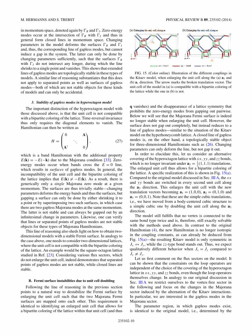
FIG. 15. (Color online) Illustration of the different couplings inthe Kitaev model, when enlarging the unit cell along the (a) a3 and(b) a1 direction. The arrow marks the broken translation vector. Theunit cell of the model in (a) is compatible with a bipartite coloring ofthe lattice while the one in (b) is not.

q vanishes) and the disappearance of a lattice symmetry thatprohibits the zero-energy modes from gapping out pairwise.Below we will see that the Majorana Fermi surface is indeedno longer stable when enlarging the unit cell. However, thesurface does not gap out completely, but instead reduces to aline of gapless modes—similar to the situation of the Kitaevmodel on the hyperhoneycomb lattice. A closed line of gaplessmodes is, on the other hand, a topologically stable objectfor three-dimensional Hamiltonians such as (26). Changingparameters can only deform the line, but not gap it out.

In order to elucidate this, let us consider an alternativecovering of the hyperoctagon lattice with xx, yy, and zz bonds,which is no longer invariant under a3 = 1

2 (1,1,1) translations.The enlarged unit cell thus allows for a bipartite coloring ofthe lattice. A specific realization of this is shown in Fig. 15(a).Compared to the original model discussed in Sec. III A, the xx

and yy bonds are switched in every second unit cell alongthe a3 direction. This enlarges the unit cell with the newtranslation vectors becoming a1 = (1,0,0), a2 = (0,1,0) anda3 = (0,0,1). Note that these are the simple cubic translations,i.e., we have moved from a body-centered cubic structure toa simple cubic one by doubling the unit cell along the a3

direction.The model still fulfills that no vertex is connected to the

same bond type twice and is, therefore, still exactly solvablewith the methods used above. In contrast to the originalHamiltonian (4), the new Hamiltonian is no longer isotropicin the coupling constants, as can already be deduced fromFig. 15(a)—the resulting Kitaev model is only symmetric inJx ↔ Jy , while the zz-type bond stands out. Thus, we expectqualitatively different behavior when Jx = Jy compared toJx = Jy .

Let us first comment on the flux sectors on the model. Itcan be shown that the constraints on the loop operators areindependent of the choice of the covering of the hyperoctagonlattice in xx, yy, and zz bonds, even though the loop operatorsthemselves change. In analogy to our original discussion inSec. III A we restrict ourselves to the vortex-free sector inthe following and focus on the changes in the Majoranasector induced by the alternation of the Kitaev interactions.In particular, we are interested in the gapless modes in theMajorana sector.

The parameter region, in which gapless modes exist,is identical to the original model, i.e., determined by the

235102-10

QUANTUM SPIN LIQUID WITH A MAJORANA FERMI . . . PHYSICAL REVIEW B 89, 235102 (2014)

FIG. 16. (Color online) Visualization of the surface vs lines ofgapless modes. On the line Jx = Jy , the model exhibits a MajoranaFermi surface—centered around (π,π,π ) as shown in panel (a). Awayfrom Jx = Jy , the surface reduces to a line, which lies in the kz =±π plane. Panels (b) and (c) show the behavior of the gapless line,when (b) increasing Jx and (c) decreasing Jx , and setting Jy = Jz =(1 − Jx)/2.

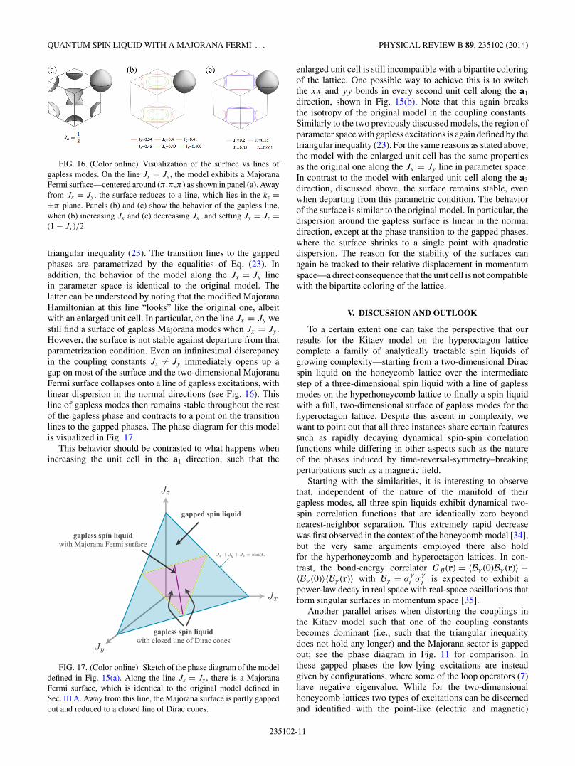
triangular inequality (23). The transition lines to the gappedphases are parametrized by the equalities of Eq. (23). Inaddition, the behavior of the model along the Jx = Jy linein parameter space is identical to the original model. Thelatter can be understood by noting that the modified MajoranaHamiltonian at this line “looks” like the original one, albeitwith an enlarged unit cell. In particular, on the line Jx = Jy westill find a surface of gapless Majorana modes when Jx = Jy .However, the surface is not stable against departure from thatparametrization condition. Even an infinitesimal discrepancyin the coupling constants Jx = Jy immediately opens up agap on most of the surface and the two-dimensional MajoranaFermi surface collapses onto a line of gapless excitations, withlinear dispersion in the normal directions (see Fig. 16). Thisline of gapless modes then remains stable throughout the restof the gapless phase and contracts to a point on the transitionlines to the gapped phases. The phase diagram for this modelis visualized in Fig. 17.

This behavior should be contrasted to what happens whenincreasing the unit cell in the a1 direction, such that the

Jz

Jx

Jy

gapped spin liquid

gapless spin liquidwith Majorana Fermi surface

J + J + J = const.

gapless spin liquidwith closed line of Dirac cones

FIG. 17. (Color online) Sketch of the phase diagram of the modeldefined in Fig. 15(a). Along the line Jx = Jy , there is a MajoranaFermi surface, which is identical to the original model defined inSec. III A. Away from this line, the Majorana surface is partly gappedout and reduced to a closed line of Dirac cones.

enlarged unit cell is still incompatible with a bipartite coloringof the lattice. One possible way to achieve this is to switchthe xx and yy bonds in every second unit cell along the a1

direction, shown in Fig. 15(b). Note that this again breaksthe isotropy of the original model in the coupling constants.Similarly to the two previously discussed models, the region ofparameter space with gapless excitations is again defined by thetriangular inequality (23). For the same reasons as stated above,the model with the enlarged unit cell has the same propertiesas the original one along the Jx = Jy line in parameter space.In contrast to the model with enlarged unit cell along the a3

direction, discussed above, the surface remains stable, evenwhen departing from this parametric condition. The behaviorof the surface is similar to the original model. In particular, thedispersion around the gapless surface is linear in the normaldirection, except at the phase transition to the gapped phases,where the surface shrinks to a single point with quadraticdispersion. The reason for the stability of the surfaces canagain be tracked to their relative displacement in momentumspace—a direct consequence that the unit cell is not compatiblewith the bipartite coloring of the lattice.

V. DISCUSSION AND OUTLOOK

To a certain extent one can take the perspective that ourresults for the Kitaev model on the hyperoctagon latticecomplete a family of analytically tractable spin liquids ofgrowing complexity—starting from a two-dimensional Diracspin liquid on the honeycomb lattice over the intermediatestep of a three-dimensional spin liquid with a line of gaplessmodes on the hyperhoneycomb lattice to finally a spin liquidwith a full, two-dimensional surface of gapless modes for thehyperoctagon lattice. Despite this ascent in complexity, wewant to point out that all three instances share certain featuressuch as rapidly decaying dynamical spin-spin correlationfunctions while differing in other aspects such as the natureof the phases induced by time-reversal-symmetry–breakingperturbations such as a magnetic field.

Starting with the similarities, it is interesting to observethat, independent of the nature of the manifold of theirgapless modes, all three spin liquids exhibit dynamical two-spin correlation functions that are identically zero beyondnearest-neighbor separation. This extremely rapid decreasewas first observed in the context of the honeycomb model [34],but the very same arguments employed there also holdfor the hyperhoneycomb and hyperoctagon lattices. In con-trast, the bond-energy correlator GB(r) = 〈Bγ (0)Bγ (r)〉 −〈Bγ (0)〉〈Bγ (r)〉 with Bγ = σ

γ

i σγ

j is expected to exhibit apower-law decay in real space with real-space oscillations thatform singular surfaces in momentum space [35].

Another parallel arises when distorting the couplings inthe Kitaev model such that one of the coupling constantsbecomes dominant (i.e., such that the triangular inequalitydoes not hold any longer) and the Majorana sector is gappedout; see the phase diagram in Fig. 11 for comparison. Inthese gapped phases the low-lying excitations are insteadgiven by configurations, where some of the loop operators (7)have negative eigenvalue. While for the two-dimensionalhoneycomb lattices two types of excitations can be discernedand identified with the point-like (electric and magnetic)

235102-11

M. HERMANNS AND S. TREBST PHYSICAL REVIEW B 89, 235102 (2014)

excitations of a Z2 gauge theory, the effective low-energytheory for the three-dimensional lattice is somewhat moreelaborate. Mandal and Surendran argued [16] that there isonly a single loop-like excitation in the gapped phases ofthe hyperhoneycomb model that exhibits nontrivial (semionic)braiding properties. Likely, a variant of their argument withsimilar conclusions can be applied to the hyperoctagon modelas well.

A clear distinction between the three spin-liquid phasesarises when considering the effect of time-reversal-symmetry–breaking perturbations such as a magnetic field. For thehoneycomb model such a perturbation is of utmost interestas the gapless Majorana modes are protected by time reversaland even an infinitesimal magnetic field (applied alongthe 111 direction) gaps out the spin liquid into a gappedtopological phase with non-Abelian vortex excitations. On amore technical level the reason for this drastic change inducedby the magnetic field can be seen in terms of the symmetryclass classification [36,37] of the underlying free (Majorana)fermion problem [38,39]. In the absence of time-reversal-symmetry breaking the model is in symmetry class BDI, whilein the presence of a magnetic field the symmetry class changesto class D. The latter allows for aZ classification of topologicalphases in two spatial dimensions. Indeed, the two bands splitby the magnetic field are characterized by Chern numbers ±1indicating the non-Abelian nature of the gapped phase.

When considering a similar line of arguments for thethree-dimensional models a different picture emerges. Asnoted earlier, the zero-energy modes of the hyperhoneycombmodel are protected by time-reversal symmetry, while theones of the hyperoctagon lattice are not. So while we expectthe gapless phase of the hyperhoneycomb model to gap outimmediately in the presence of a magnetic field, this is farfrom obvious for the zero-energy modes of the hyperoctagonmodel because the spectrum is robust against any two-fermionterm that does not break translation symmetry. Independentof whether a gap opens in the spectrum, it still holds thatthe symmetry class of the underlying free (Majorana) fermionmodel changes from class BDI to class D in the presence of atime-reversal–symmetry–breaking term. However, in contrastto its two-dimensional counterpart, symmetry class D doesnot harbor any topological phases in three dimensions [36,37].As a consequence, the three-dimensional systems cannot bedriven into a (non-Abelian) topological phase by applying amagnetic field (or any other time-reversal-symmetry–breakingperturbation). However, one might still be able to employ ideassimilar to those used by Ryu in Ref. [40] to stabilize a nontrivialtopological phase by introducing additional (orbital) degreesof freedom such that the augmented model can be reformulatedas a free-fermion model in symmetry class DIII. The latter doeshave a Z classification in three dimensions and, thus, allowsfor three-dimensional analogs of the topological phase in thehoneycomb model.

1. Thermodynamic signatures of spin liquid

Finally, an interesting perspective emerges when recastingour results in the terminology conventionally used to char-acterize various spin-liquid states [1]. In this language, wehave discovered a spin liquid with a spinon Fermi surface that

covers an extensive two-dimensional manifold in momentumspace. The quest to identify magnetic systems harboringsuch spinon Fermi surfaces has typically inspired theoriststo consider a slave-fermion approach where the fermioninteracts with a fluctuating U(1) gauge field—a situation thatis notoriously hard to track analytically and any progresscoming at the expense of compromises on the level of variousdecoupling or mean-field approaches. This situation should becontrasted to the current situation where we have stumbledupon a system with a spinon Fermi surface with a muchsimpler and analytically exact description in terms of Majoranafermions interacting with a staticZ2 gauge field. However, it isimportant to note that this difference is not a mere conceptualone, but one that has direct implications for thermodynamicobservables such as the specific-heat coefficient C/T . For aU(1) spin liquid the specific heat diverges as

C(T ) ∝ T ln(1/T ),

i.e., the specific-heat coefficient γ = C/T diverges logarith-mically at low temperatures [41]. For our case of a spinonFermi surface emerging from Majorana fermions interactingwith a Z2 gauge field, we find

C(T ) ∝ T ,

i.e., the specific-heat coefficient γ goes to a constant at lowtemperatures. Finally, this situation should be contrasted tothe spin liquid with a Fermi line, as it was found for thehyperhoneycomb lattice, where the specific heat grows as [17]

C(T ) ∝ T 2,

i.e., the specific-heat coefficient γ vanishes in the limitof T → 0. Remarkably enough, this implies that a simplethermodynamic experiment could immediately distinguishthese three seemingly equally exotic spin liquids.

Returning to the perspective of the free (Majorana) fermionsystem underlying our gapless spin liquid, there is one obviousbouquet of questions that we have not addressed in themanuscript at hand—namely, the various pairing instabilitiesthat the Fermi surface of our system might exhibit. Onemight be particularly interested in asking what instabilities canbe induced by additional interactions such as a Heisenbergexchange argued to accompany the Kitaev interactions inany microscopic description of iridate compounds [6,7]. Theeffective description of the hyperoctagon model in termsof spinless fermions suggests p-wave pairing as the naturalcandidate for opening a gap. Interaction terms of this typecan indeed arise in a perturbative analysis of the Heisenbergexchange. The question of whether or not these terms lead toa collapse of the Majorana Fermi surface or even gap out allMajorana modes in the system is left for future work.

ACKNOWLEDGMENTS

We thank A. Akhmerov, A. Altland, P. Becker-Bohaty,S. Parameswaran, F. Pollmann, and especially A. Rosch forinsightful discussions. S.T. acknowledges the hospitality of theAspen Center for Physics where some of the ideas underlyingthis manuscript were perceived. S.T. is indebted to L. Balentsfor a beginner’s guide to three-dimensional printing. Weacknowledge partial support from SFB TR 12 of the DFG.

235102-12

QUANTUM SPIN LIQUID WITH A MAJORANA FERMI . . . PHYSICAL REVIEW B 89, 235102 (2014)

APPENDIX A: POSSIBLE MAGNETIC MATERIALSIN SPACE GROUP I4132

In this Appendix, we want to expand our discussion ofpossible magnetic materials candidates in space group I4132(no. 214). The guiding idea in our analysis is to put thespace group symmetries of I4132 to work and look for variouspossible ways to fill the interstitial sites between the networkof edge-sharing IrO6 cages as illustrated in Fig. 5 of themain text. In addition, we have to take into account that thefundamental building blocks of IrO3 have valency −2 and assuch are looking for interstitial fillings that allow to chemicallycompensate this valence.

1. Space group symmetries

Let us first consider the effect of the space group symme-tries. There are in total 48 symmetry operations in the spacegroup I4132. A generic point in the cubic cell is, thus, mappedto in total 48 distinct points; the set of these points will, inthe following, often be labeled by a single representative.However, there are several high-symmetry points, respectivelylines in the cubic cell, which are mapped to far fewer points. Intotal, we can distinguish five types of lattice points, accordingto the number of distinct lattice points that can be reached bythe symmetry operations:

(i) The lattice point is mapped to eight distinct lattice pointsin the unit cell. This is possible in two inequivalent ways. Theresulting points form the two chiralities of the hyperoctagonlattice. The representatives of the two possibilities are 1

8 (1,1,1)and − 1

8 (1,1,1). In the main text, we chose the hyperoctagonlattice generated by 1

8 (1,1,1); thus, in the following we placethe iridium atoms on this set of sites.

(ii) The lattice point is mapped to 12 distinct lattice pointsin the unit cell. This is again possible in two inequivalent ways.The representatives are given by (0, 1

4 , 18 ) and (0, 1

4 , 58 ). These

sites form effective lattices, which are deformations of thetwo chiral versions of the hyperkagome. In fact, they can beidentified as the medial lattices of the two chiral hyperoctagonlattices in (i).

(iii) The lattice point is mapped to 16 distinct lattice pointsin the unit cell. There are infinitely many such possibilities, aslong as the representative is chosen on the line (x,x,x) [exceptthe high-symmetry points already listed in (i)].

(iv) The lattice point is mapped to 24 distinct lattice pointsin the unit cell. There are many high-symmetry lines in thecubic unit cell which lead to this behavior. The oxygen sitesare an example for this type of lattice point—represented by18 (1, − 1,1).

(v) The lattice point is mapped to 48 distinct lattice pointsin the unit cell, which applies to all lattice points that do notlie on one of the above mentioned high-symmetry lines.

2. Possible chemical compositions

This structure, imposed by the symmetry group, severelyrestricts the composition of possible compounds. Assumingthe presence of edge-sharing IrO6 cages, we note that theabove analysis implies that there are eight IrO3 in a cubicunit cell. Thus, the remaining atoms must compensate a totalvalency of −16. The latter can, for instance, be achieved by

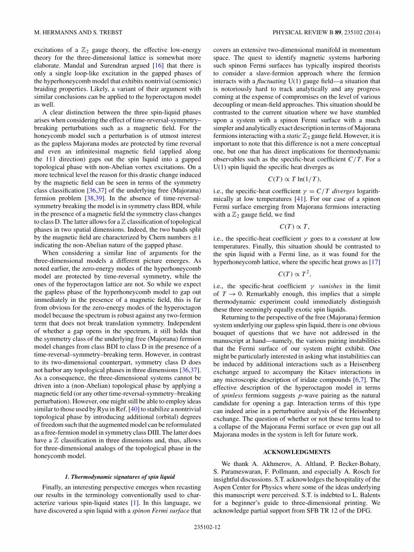
FIG. 18. (Color online) Two possibilities of placing atoms on theinterstitial sites in the IrO3 structures, indicated by the gray octahedra.Panel (a) shows the crystal structure by placing atoms of valency +2on the sites of type (i) (see text). In panel (b), atoms with valency+1 are placed on sites of type (iii), which are generated by therepresentative (0,0,0).

placing eight atoms with valency +2 on the remaining set ofsites of type (i). The resulting compound is of the form AIrO3,where A is one of the alkaline-earth-metal elements Ca, Sr,or Ba. Another possibility is to place 16 atoms of valency +1on the sites of type (iii). This results in a material of the typeA2IrO3, where A is one of the alkali-metal atoms Na or Li. Theresulting crystal structures for both possibilities are visualizedin Fig. 18.

APPENDIX B: KITAEV MODEL ON HYPERHONEYCOMBLATTICE

To complement our discussion of the Kitaev model onthe hyperoctagon lattice, we present a brief, self-containedsummary of the Kitaev model on the hyperhoneycomb lattice,an alternative trivalent three-dimensional (3D) lattice, inthis Appendix. For clarity, we use similar notations andconventions as in the main text, but emphasize that in doingso we also closely follow the original solution of the Kitaevmodel on the hyperhoneycomb lattice as discussed in somedetail in Ref. [15].

1. Hyperhoneycomb lattice

The hyperhoneycomb lattice is an alternative 3D latticewith a trivalent lattice structure which is illustrated in Fig. 19.Its elementary building blocks are zigzag chains running alongthe crystallographic b and c axes, which are coupled along thea axis. Its crystal structure can be classified as a face-centered

235102-13

M. HERMANNS AND S. TREBST PHYSICAL REVIEW B 89, 235102 (2014)

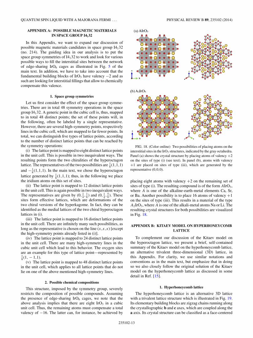
FIG. 19. (Color online) The hyperhoneycomb lattice. The four-site unit cell and translation vectors are indicated. Green bondscorrespond to xx couplings, red bonds to yy coupling, and bluebonds to zz coupling.

orthorhombic lattice of space group number 70. Of particularimportance for our discussion is the fact that it is not spatiallyisotropic as is the hyperoctagon lattice, but has one “preferred”direction—the a direction in Fig. 19.

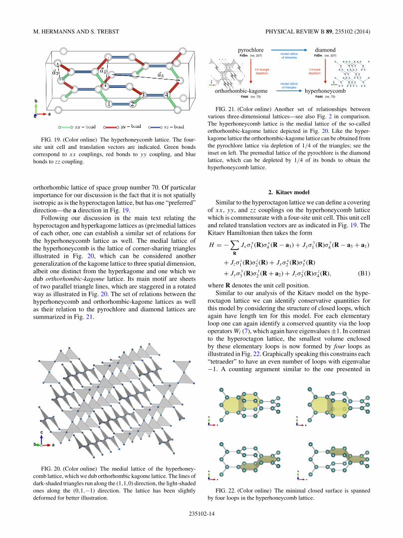
Following our discussion in the main text relating thehyperoctagon and hyperkagome lattices as (pre)medial latticesof each other, one can establish a similar set of relations forthe hyperhoneycomb lattice as well. The medial lattice ofthe hyperhoneycomb is the lattice of corner-sharing trianglesillustrated in Fig. 20, which can be considered anothergeneralization of the kagome lattice to three spatial dimension,albeit one distinct from the hyperkagome and one which wedub orthorhombic-kagome lattice. Its main motif are sheetsof two parallel triangle lines, which are staggered in a rotatedway as illustrated in Fig. 20. The set of relations between thehyperhoneycomb and orthorhombic-kagome lattices as wellas their relation to the pyrochlore and diamond lattices aresummarized in Fig. 21.

FIG. 20. (Color online) The medial lattice of the hyperhoney-comb lattice, which we dub orthorhombic kagome lattice. The lines ofdark-shaded triangles run along the (1,1,0) direction, the light-shadedones along the (0,1,−1) direction. The lattice has been slightlydeformed for better illustration.

pyrochlore

orthorhombic-kagome

diamond

hyperhoneycomb

medial latticeof tetraedra

medial latticeof triangles

1/4 triangledepletion

1/4 bonddepletion

Fddd (no. 70) Fddd (no. 70)

Fd3m (no. 227) Fd3m (no. 227)

FIG. 21. (Color online) Another set of relationships betweenvarious three-dimensional lattices—see also Fig. 2 in comparison.The hyperhoneycomb lattice is the medial lattice of the so-calledorthorhombic-kagome lattice depicted in Fig. 20. Like the hyper-kagome lattice the orthorhombic-kagome lattice can be obtained fromthe pyrochlore lattice via depletion of 1/4 of the triangles; see theinset on left. The premedial lattice of the pyrochlore is the diamondlattice, which can be depleted by 1/4 of its bonds to obtain thehyperhoneycomb lattice.

2. Kitaev model

Similar to the hyperoctagon lattice we can define a coveringof xx, yy, and zz couplings on the hyperhoneycomb latticewhich is commensurate with a four-site unit cell. This unit celland related translation vectors are as indicated in Fig. 19. TheKitaev Hamiltonian then takes the form

H = −∑

R

Jxσx1 (R)σx

4 (R − a3) + Jyσy

1 (R)σy

4 (R − a3 + a1)

+ Jzσz1 (R)σ z

2 (R) + Jxσx2 (R)σx

3 (R)

+ Jyσy

3 (R)σy

2 (R + a2) + Jzσz3 (R)σ z

4 (R), (B1)

where R denotes the unit cell position.Similar to our analysis of the Kitaev model on the hype-

roctagon lattice we can identify conservative quantities forthis model by considering the structure of closed loops, whichagain have length ten for this model. For each elementaryloop one can again identify a conserved quantity via the loopoperators Wl (7), which again have eigenvalues ±1. In contrastto the hyperoctagon lattice, the smallest volume enclosedby these elementary loops is now formed by four loops asillustrated in Fig. 22. Graphically speaking this constrains each“tetraeder” to have an even number of loops with eigenvalue−1. A counting argument similar to the one presented in

FIG. 22. (Color online) The minimal closed surface is spannedby four loops in the hyperhoneycomb lattice.

235102-14

QUANTUM SPIN LIQUID WITH A MAJORANA FERMI . . . PHYSICAL REVIEW B 89, 235102 (2014)

our main analysis in Sec. III B 1 shows that there are 22N

different flux sectors, where N is the number of unit cells.Numerical simulations [15,18] indicate that the ground stateindeed resides in the zero-flux sector, which is why we restrictthe following discussion to this sector.

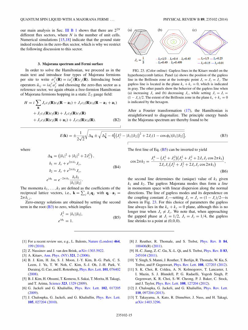
3. Majorana spectrum and Fermi surface

In order to solve the Hamiltonian, we proceed as in themain text and introduce four types of Majorana fermionsper site to write σ

γ

j (R) = iaγ

j (R)cj (R). Introducing bondoperators uij = ia

γ

i aγ

j and choosing the zero-flux sector as areference sector, we again obtain a free-fermion Hamiltonianof Majorana fermions hopping in a static Z2 gauge field:

H = i∑

R

Jxc1(R)c4(R − a3) + Jyc1(R)c4(R − a3 + a1)

+ Jzc1(R)c2(R) + Jxc2(R)c3(R)

+ Jyc3(R)c2(R + a2) + Jzc3(R)c4(R). (B2)

FIG. 23. (Color online) Gapless lines in the Kitaev model on thehyperhoneycomb lattice. Panel (a) shows the position of the gaplessline in the Brillouin zone at the isotropic point Jx = Jy = Jz. Thegapless line is located in the plane kx + ky = 0, which is indicatedin gray. The other panels show the behavior of the gapless line when(a) increasing Jx and (b) decreasing Jx , while setting Jy = Jz =(1 − Jx)/2. The extent of the Brillouin zone in the plane kx + ky = 0is indicated by the hexagon.

After a Fourier transformation (17), the Hamiltonian isstraightforward to diagonalize. The principle energy bandsin the Majorana spectrum are thereby found to be

E(k) = ± 1

2√

2

√�k ±

√�2

k − 4[(

J 2z − |δ1||δ2|

)2 + 2Jz(1 − cos φk)|δ1||δ2|], (B3)

where

�k = (|δ1|2 + |δ2|2 + 2J 2z

),

δ1 = Jx + e2πik1Jy,(B4)

δ2 = Jx + e2πik2Jy,

eiφk = e−2πik3δ1δ2

|δ1||δ2| .The momenta k1, . . . ,k3 are defined as the coefficients of thereciprocal lattice vectors, i.e., k = ∑

j kj qj with qi · aj =2πδi,j .

Zero-energy solutions are obtained by setting the secondterm in the root (B3) to zero, which implies

J 2z = |δ1||δ2|,

(B5)eiφk = 1.

The first line of Eq. (B5) can be inverted to yield

cos 2πk2 = J 4z − (

J 2x + J 2

y

)(J 2

x + J 2y + 2JxJy cos 2πk1

)2JxJy

(J 2

x + J 2y + 2JxJy cos 2πk1

) ,

(B6)

the second line determines the (unique) value of k3 givenk1 and k2. The gapless Majorana modes thus form a linein momentum space with linear dispersion along the normaldirections. The line of gapless modes and its dependence onthe coupling constant Jz—setting Jx = Jy = (1 − Jz)/2—isshown in Fig. 23. For this choice of parameters the gaplessline always lies in the kx + ky = 0 plane, although this is nolonger true when Jx = Jy . We note that, when approachingthe gapped phase at Jz = 1/2, Jx = Jy = 1/4, the gaplessline shrinks to a point at (0,0,0).

[1] For a recent review see, e.g., L. Balents, Nature (London) 464,199 (2010).

[2] Z. Nussinov and J. van den Brink, arXiv:1303.5922.[3] A. Kitaev, Ann. Phys. (NY) 321, 2 (2006).[4] B. J. Kim, H. Jin, S. J. Moon, J.-Y. Kim, B.-G. Park, C. S.

Leem, J. Yu, T. W. Noh, C. Kim, S.-J. Oh, J.-H. Park, V.Durairaj, G. Cao, and E. Rotenberg, Phys. Rev. Lett. 101, 076402(2008).

[5] B. J. Kim, H. Ohsumi, T. Komesu, S. Sakai, T. Morita, H. Takagi,and T. Arima, Science 323, 1329 (2009).

[6] G. Jackeli and G. Khaliullin, Phys. Rev. Lett. 102, 017205(2009).

[7] J. Chaloupka, G. Jackeli, and G. Khaliullin, Phys. Rev. Lett.105, 027204 (2010).

[8] J. Reuther, R. Thomale, and S. Trebst, Phys. Rev. B 84,100406(R) (2011).

[9] H.-C. Jiang, Z.-C. Gu, X.-L. Qi, and S. Trebst, Phys. Rev. B 83,245104 (2011).

[10] Y. Singh, S. Manni, J. Reuther, T. Berlijn, R. Thomale, W. Ku, S.Trebst, and P. Gegenwart, Phys. Rev. Lett. 108, 127203 (2012).

[11] S. K. Choi, R. Coldea, A. N. Kolmogorov, T. Lancaster, I.I. Mazin, S. J. Blundell, P. G. Radaelli, Yogesh Singh, P.Gegenwart, K. R. Choi, S.-W. Cheong, P. J. Baker, C. Stock,and J. Taylor, Phys. Rev. Lett. 108, 127204 (2012).

[12] J. Chaloupka, G. Jackeli, and G. Khaliullin, Phys. Rev. Lett.110, 097204 (2013).

[13] T. Takayama, A. Kato, R. Dinnebier, J. Nuss, and H. Takagi,arXiv:1403.3296.

235102-15

M. HERMANNS AND S. TREBST PHYSICAL REVIEW B 89, 235102 (2014)

[14] After completion of this work, another crystalline form ofLi2IrO3 realizing a slightly different three-dimensional, trico-ordinated, honeycomb-like lattice structure of the Ir ions wasreported in Ref. [42].

[15] S. Mandal and N. Surendran, Phys. Rev. B 79, 024426 (2009).[16] S. Mandal and N. Surendran, arXiv:1101.3718.[17] EricKin-Ho Lee, R. Schaffer, S. Bhattacharjee, and Y. B. Kim,

Phys. Rev. B 89, 045117 (2014).[18] I. Kimchi, J. G. Analytis, and A. Vishwanath, arXiv:1309.1171.[19] S. B. Lee, EricKin-Ho Lee, A. Paramekanti, and Y. B. Kim,

Phys. Rev. B 89, 014424 (2014).[20] For the convenience of the inclined reader we provide a

VESTA [43] visualization file of the hyperoctagon lattice in theSupplemental Material [44].

[21] R. Si and Y. Yu, Nucl. Phys. B 803, 428 (2008).[22] Further generalizations of the Kitaev models also to lattices with

higher vertex coordination number, in particular the kagome,triangular, hyperkagome, and pyrochlore lattices have beenstudied [45–47]. It should, however, be noted that it is preciselythe higher coordination number of the vertices in these latticeswhich prohibits following the same analytical route that can beused for the trivalent ones.

[23] S. Yang, D. L. Zhou, and C. P. Sun, Phys. Rev. B 76, 180404(R)(2007); G. Kells, J. Kailasvuori, J. Slingerland, and J. Vala, NewJ. Phys. 13, 095014 (2011).

[24] Y. Okamoto, M. Nohara, H. Aruga-Katori, and H. Takagi, Phys.Rev. Lett. 99, 137207 (2007).

[25] C. Zheng, O. Oeckler, H. Mattausch, and A. Simon, Z. Anorg.Allg. Chem. 627, 2151 (2001).

[26] E. Morosan, J. A. Fleitman, Q. Huang, J. W. Lynn, Y. Chen, X.Ke, M. L. Dahlberg, P. Schiffer, C. R. Craley, and R. J. Cava,Phys. Rev. B 77, 224423 (2008).

[27] K. Ohgushi, H. Gotou, T. Yagi, Y. Kiuchi, F. Sakai, and Y. Ueda,Phys. Rev. B 74, 241104(R) (2006).

[28] G. Cao, J. E. Crow, R. P. Guertin, P. F. Henning, C. C. Homes,M. Strongin, D. N. Basov, and E. Lochner, Solid State Commun.113, 657 (2000).

[29] G. Cao, V. Durairaj, S. Chikara, L. E. DeLong, S. Parkin, and P.Schlottmann, Phys. Rev. B 76, 100402(R) (2007).

[30] The relative sign for the two alternative definitions of theloop operator, and subsequent “freedom” to define magneticflux, appears also for other trivalent lattices; for instance, thetwo-dimensional square-octagon lattice. Using the operator Wl

[Eq. (7)] to define the flux ensures that the notion of 0/π -fluxper plaquette is consistent with the one used by Lieb [31]. Inparticular, the ground state of the square-octagon lattice residesin the full-flux sector according to Lieb’s theorem, because theloops have lengths four and eight, respectively.

[31] E. H. Lieb, Phys. Rev. Lett. 73, 2158 (1994).[32] See also the related work by A. M. Tsvelik, Phys. Rev. Lett. 69,

2142 (1992).[33] The zeros on the diagonal are, in fact, not important for the

argument.[34] G. Baskaran, Saptarshi Mandal, and R. Shankar, Phys. Rev. Lett.

98, 247201 (2007).[35] Similar behavior was found in H.-H. Lai and O. I. Motrunich,

Phys. Rev. B 83, 155104 (2011).[36] A. P. Schnyder, S. Ryu, A. Furusaki, and A. W. W. Ludwig,

Phys. Rev. B 78, 195125 (2008).[37] A. Kitaev, AIP Conf. Proc. 1134, 22 (2009).[38] M. R. Zirnbauer, J. Math. Phys. 37, 4986 (1996).[39] A. Altland and M. R. Zirnbauer, Phys. Rev. B 55, 1142 (1997).[40] S. Ryu, Phys. Rev. B 79, 075124 (2009).[41] T. Holstein, R. Norton, and P. Pincus, Phys. Rev. B 8, 2649

(1973); M. Yu. Reizer, ibid. 40, 11571 (1989).[42] K. A. Modic et al., arXiv:1402.3254.[43] K. Momma and F. Izumi, J. Appl. Crystallogr. 44, 1272 (2011).[44] See Supplemental Material at http://link.aps.org/supplemental/

10.1103/PhysRevB.89.235102 for details.[45] I. Kimchi and A. Vishwanath, Phys. Rev. B 89, 014414 (2014).[46] I. Rousochatzakis, U. K. Rossler, J. van den Brink, and M.

Daghofer, arXiv:1209.5895.[47] M. Becker, M. Hermanns, B. Bauer, M. Garst, and S. Trebst

(unpublished).

235102-16