Quantum Optical Phase Estimation byPhase-Locked Loops

Mankei Tsang, Jeffrey H. Shapiro, and Seth Lloyd

mankei@mit.edu

xQIT, MIT

Quantum Optical Phase Estimation by Phase-Locked Loops – p.1/22

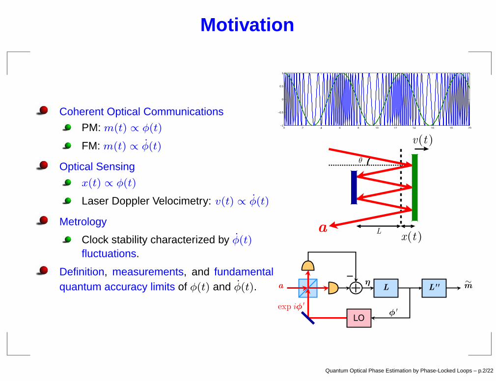
Motivation

Coherent Optical Communications

PM: m(t) ∝ φ(t)

FM: m(t) ∝ φ(t)

Optical Sensing

x(t) ∝ φ(t)

Laser Doppler Velocimetry: v(t) ∝ φ(t)

Metrology

Clock stability characterized by φ(t)

fluctuations.

Definition, measurements, and fundamentalquantum accuracy limits of φ(t) and φ(t).

0 2 4 6 8 10 12 14 16 18 20−1

−0.5

0

0.5

1

Quantum Optical Phase Estimation by Phase-Locked Loops – p.2/22

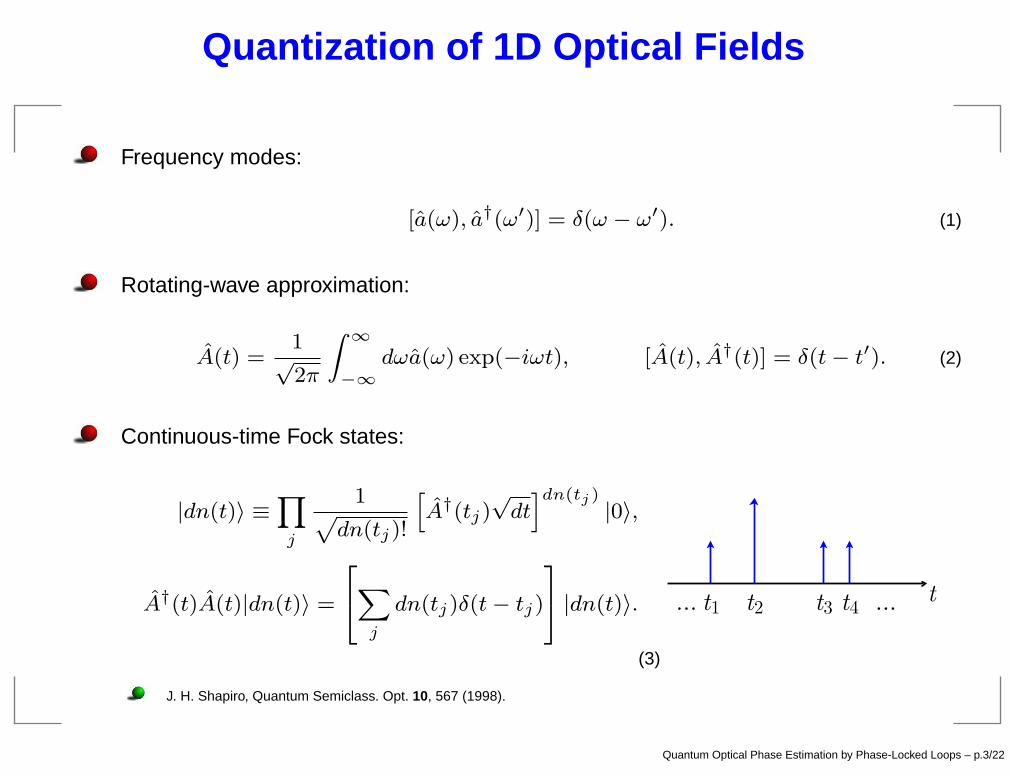
Quantization of 1D Optical Fields

Frequency modes:

[a(ω), a†(ω′)] = δ(ω − ω′). (1)

Rotating-wave approximation:

A(t) =1√2π

Z ∞

−∞

dωa(ω) exp(−iωt), [A(t), A†(t)] = δ(t− t′). (2)

Continuous-time Fock states:

|dn(t)〉 ≡Y

j

1pdn(tj)!

hA†(tj)

√dtidn(tj)

|0〉,

A†(t)A(t)|dn(t)〉 =

24X

j

dn(tj)δ(t− tj)

35 |dn(t)〉.

(3)

J. H. Shapiro, Quantum Semiclass. Opt. 10, 567 (1998).

Quantum Optical Phase Estimation by Phase-Locked Loops – p.3/22

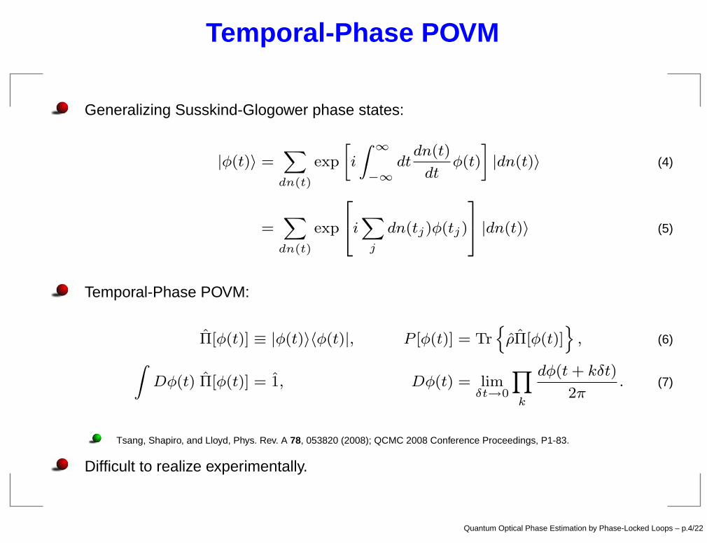
Temporal-Phase POVM

Generalizing Susskind-Glogower phase states:

|φ(t)〉 =X

dn(t)

exp

»i

Z ∞

−∞

dtdn(t)

dtφ(t)

–|dn(t)〉 (4)

=X

dn(t)

exp

24iX

j

dn(tj)φ(tj)

35 |dn(t)〉 (5)

Temporal-Phase POVM:

Π[φ(t)] ≡ |φ(t)〉〈φ(t)|, P [φ(t)] = TrnρΠ[φ(t)]

o, (6)

ZDφ(t) Π[φ(t)] = 1, Dφ(t) = lim

δt→0

Y

k

dφ(t+ kδt)

2π. (7)

Tsang, Shapiro, and Lloyd, Phys. Rev. A 78, 053820 (2008); QCMC 2008 Conference Proceedings, P1-83.

Difficult to realize experimentally.

Quantum Optical Phase Estimation by Phase-Locked Loops – p.4/22

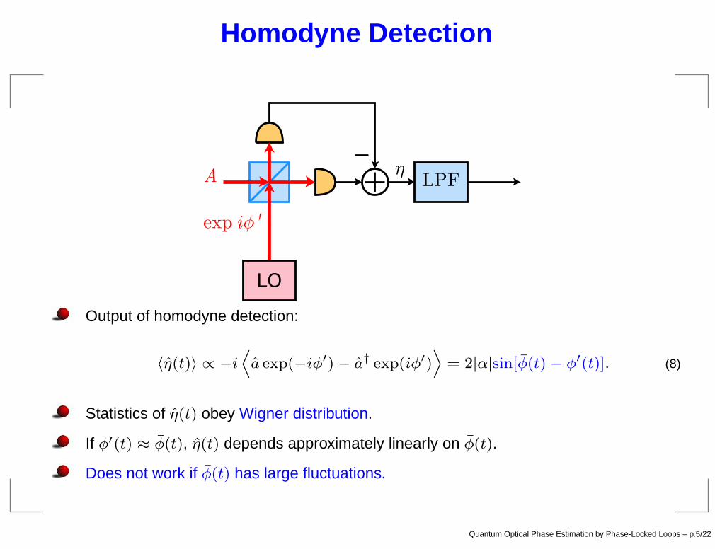
Homodyne Detection

Output of homodyne detection:

〈η(t)〉 ∝ −iDa exp(−iφ′) − a† exp(iφ′)

E= 2|α|sin[φ(t) − φ′(t)]. (8)

Statistics of η(t) obey Wigner distribution.

If φ′(t) ≈ φ(t), η(t) depends approximately linearly on φ(t).

Does not work if φ(t) has large fluctuations.

Quantum Optical Phase Estimation by Phase-Locked Loops – p.5/22

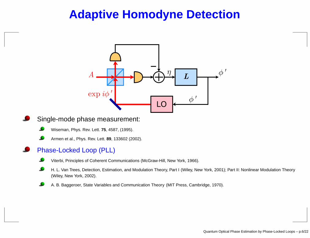
Adaptive Homodyne Detection

Single-mode phase measurement:

Wiseman, Phys. Rev. Lett. 75, 4587, (1995).

Armen et al., Phys. Rev. Lett. 89, 133602 (2002).

Phase-Locked Loop (PLL)Viterbi, Principles of Coherent Communications (McGraw-Hill, New York, 1966).

H. L. Van Trees, Detection, Estimation, and Modulation Theory, Part I (Wiley, New York, 2001); Part II: Nonlinear Modulation Theory(Wiley, New York, 2002).

A. B. Baggeroer, State Variables and Communication Theory (MIT Press, Cambridge, 1970).

Quantum Optical Phase Estimation by Phase-Locked Loops – p.6/22

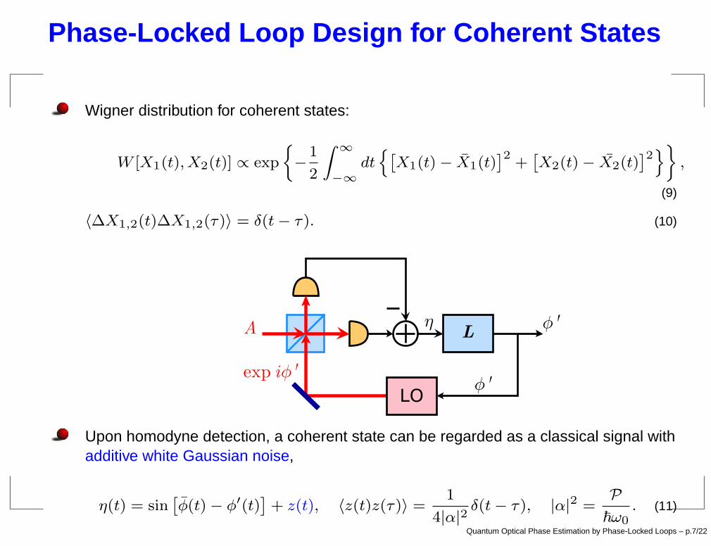
Phase-Locked Loop Design for Coherent States

Wigner distribution for coherent states:

W [X1(t), X2(t)] ∝ exp

−1

2

Z ∞

−∞

dtnˆX1(t) − X1(t)

˜2+ˆX2(t) − X2(t)

˜2off,

(9)

〈∆X1,2(t)∆X1,2(τ)〉 = δ(t− τ). (10)

Upon homodyne detection, a coherent state can be regarded as a classical signal withadditive white Gaussian noise,

η(t) = sinˆφ(t) − φ′(t)

˜+ z(t), 〈z(t)z(τ)〉 =

1

4|α|2 δ(t− τ), |α|2 =P

~ω0. (11)

Quantum Optical Phase Estimation by Phase-Locked Loops – p.7/22

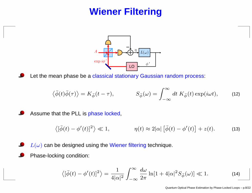
Wiener Filtering

Let the mean phase be a classical stationary Gaussian random process:

˙φ(t)φ(τ)

¸= Kφ(t− τ), Sφ(ω) =

Z ∞

−∞

dt Kφ(t) exp(iωt), (12)

Assume that the PLL is phase locked,

˙[φ(t) − φ′(t)]2

¸≪ 1, η(t) ≈ 2|α|

ˆφ(t) − φ′(t)

˜+ z(t). (13)

L(ω) can be designed using the Wiener filtering technique.

Phase-locking condition:

˙[φ(t) − φ′(t)]2

¸=

1

4|α|2Z ∞

−∞

dω

2πln[1 + 4|α|2Sφ(ω)] ≪ 1. (14)

Quantum Optical Phase Estimation by Phase-Locked Loops – p.8/22

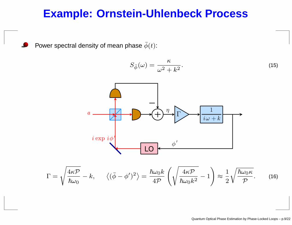
Example: Ornstein-Uhlenbeck Process

Power spectral density of mean phase φ(t):

Sφ(ω) =κ

ω2 + k2. (15)

Γ =

s4κP~ω0

− k,˙(φ− φ′)2

¸=

~ω0k

4P

s4κP

~ω0k2− 1

!≈ 1

2

r~ω0κ

P . (16)

Quantum Optical Phase Estimation by Phase-Locked Loops – p.9/22

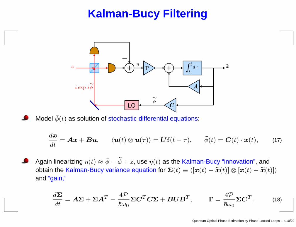
Kalman-Bucy Filtering

Model φ(t) as solution of stochastic differential equations:

dx

dt= Ax + Bu, 〈u(t) ⊗ u(τ)〉 = Uδ(t− τ), φ(t) = C(t) · x(t), (17)

Again linearizing η(t) ≈ φ− eφ+ z, use η(t) as the Kalman-Bucy “innovation”, andobtain the Kalman-Bucy variance equation for Σ(t) ≡ 〈[x(t) − ex(t)] ⊗ [x(t) − ex(t)]〉and “gain,”

dΣ

dt= AΣ + ΣA

T − 4P~ω0

ΣCT

CΣ + BUBT , Γ =

4P~ω0

ΣCT . (18)

Quantum Optical Phase Estimation by Phase-Locked Loops – p.10/22

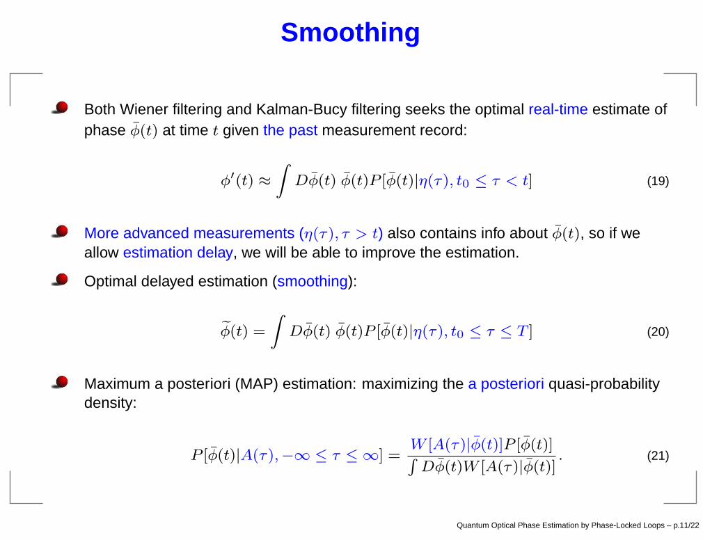
Smoothing

Both Wiener filtering and Kalman-Bucy filtering seeks the optimal real-time estimate ofphase φ(t) at time t given the past measurement record:

φ′(t) ≈ZDφ(t) φ(t)P [φ(t)|η(τ), t0 ≤ τ < t] (19)

More advanced measurements (η(τ), τ > t) also contains info about φ(t), so if weallow estimation delay, we will be able to improve the estimation.

Optimal delayed estimation (smoothing):

eφ(t) =

ZDφ(t) φ(t)P [φ(t)|η(τ), t0 ≤ τ ≤ T ] (20)

Maximum a posteriori (MAP) estimation: maximizing the a posteriori quasi-probabilitydensity:

P [φ(t)|A(τ),−∞ ≤ τ ≤ ∞] =W [A(τ)|φ(t)]P [φ(t)]RDφ(t)W [A(τ)|φ(t)]

. (21)

Quantum Optical Phase Estimation by Phase-Locked Loops – p.11/22

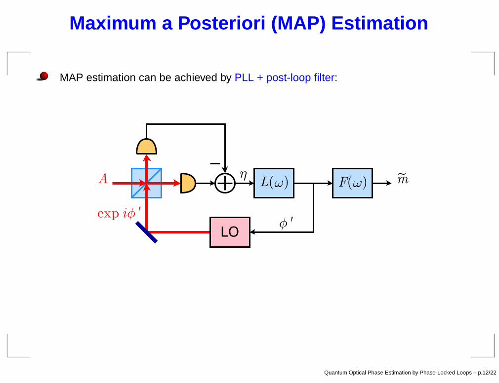
Maximum a Posteriori (MAP) Estimation

MAP estimation can be achieved by PLL + post-loop filter:

Quantum Optical Phase Estimation by Phase-Locked Loops – p.12/22

Example: Ornstein-Uhlenbeck Process

For phase modulation, let φ(t) = βm(t).

0 1 2 3 4 5 6 7 8 9 100

0.1

0.2

0.3

0.4

0.5

0.6

0.7

0.8

0.9

1

td

1/γ

F (ω) =k + γ

−iω + γexp(−iωtd), γ ≡

„4κβ2P

~ω0+ k2

«1/2

. (22)

“Irreducible Error”:

˙(m− em)2

¸=

Z ∞

−∞

dω

2π

Sm(ω)

4|α|2β2Sm(ω) + 1=

κ

2γ≈ 1

4β

r~ω0κ

P (23)

∼ 3 dB better than Wiener or Kalman-Bucy filtering.

Quantum Optical Phase Estimation by Phase-Locked Loops – p.13/22

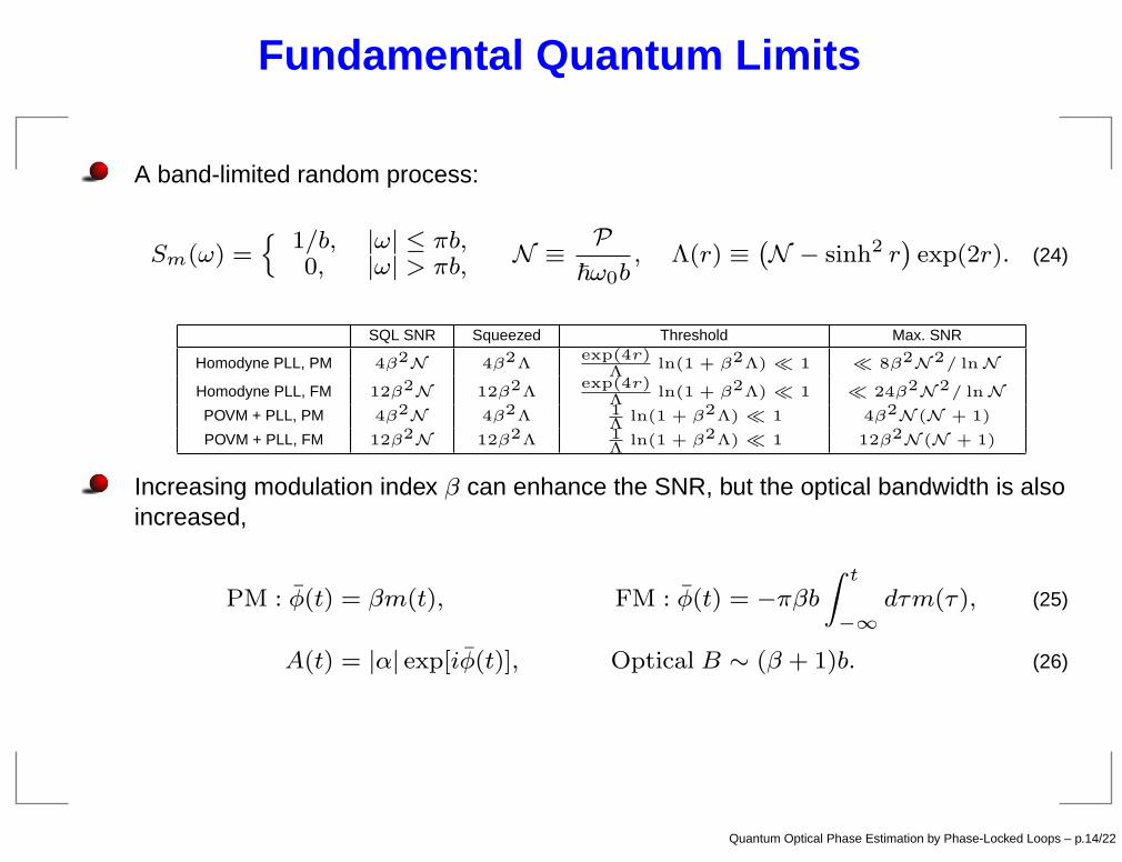
Fundamental Quantum Limits

A band-limited random process:

Sm(ω) =n

1/b, |ω| ≤ πb,0, |ω| > πb, N ≡ P

~ω0b, Λ(r) ≡

`N − sinh2 r

´exp(2r). (24)

SQL SNR Squeezed Threshold Max. SNR

Homodyne PLL, PM 4β2N 4β2Λexp(4r)

Λln(1 + β2Λ) ≪ 1 ≪ 8β2N2/ ln N

Homodyne PLL, FM 12β2N 12β2Λexp(4r)

Λln(1 + β2Λ) ≪ 1 ≪ 24β2N2/ ln N

POVM + PLL, PM 4β2N 4β2Λ 1Λ

ln(1 + β2Λ) ≪ 1 4β2N(N + 1)

POVM + PLL, FM 12β2N 12β2Λ 1Λ

ln(1 + β2Λ) ≪ 1 12β2N(N + 1)

Increasing modulation index β can enhance the SNR, but the optical bandwidth is alsoincreased,

PM : φ(t) = βm(t), FM : φ(t) = −πβbZ t

−∞

dτm(τ), (25)

A(t) = |α| exp[iφ(t)], Optical B ∼ (β + 1)b. (26)

Quantum Optical Phase Estimation by Phase-Locked Loops – p.14/22

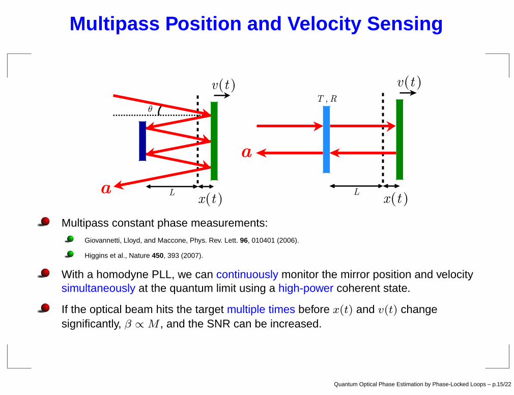
Multipass Position and Velocity Sensing

Multipass constant phase measurements:Giovannetti, Lloyd, and Maccone, Phys. Rev. Lett. 96, 010401 (2006).

Higgins et al., Nature 450, 393 (2007).

With a homodyne PLL, we can continuously monitor the mirror position and velocitysimultaneously at the quantum limit using a high-power coherent state.

If the optical beam hits the target multiple times before x(t) and v(t) changesignificantly, β ∝M , and the SNR can be increased.

Quantum Optical Phase Estimation by Phase-Locked Loops – p.15/22

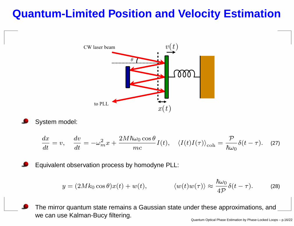
Quantum-Limited Position and Velocity Estimation

System model:

dx

dt= v,

dv

dt= −ω2

mx+2M~ω0 cos θ

mcI(t), 〈I(t)I(τ)〉coh =

P~ω0

δ(t− τ). (27)

Equivalent observation process by homodyne PLL:

y = (2Mk0 cos θ)x(t) + w(t), 〈w(t)w(τ)〉 ≈ ~ω0

4P δ(t− τ). (28)

The mirror quantum state remains a Gaussian state under these approximations, andwe can use Kalman-Bucy filtering.

Quantum Optical Phase Estimation by Phase-Locked Loops – p.16/22

Kalman-Bucy Filtering Errors

The Kalman-Bucy covariances at steady state t→ ∞ are

˙∆x2

¸=

~

2mωm

√2

Q

h(1 +Q2)1/2 − 1

i1/2, (29)

1

2〈∆x∆v + ∆v∆x〉 =

~

2m

1

Q

h(1 +Q2)1/2 − 1

i, (30)

˙∆v2

¸=

~ωm

2m

√2

Q

h(1 +Q2)1/2 − 1

i1/2(1 +Q2)1/2, (31)

Q ≡ 8M2ω0P cos2 θ

mω2mc

2. (32)

Previously derived using a general QND measurement model in

Belavkin and Staszewski, Phys. Lett. A 140, 359 (1989).

Doherty et al., Phys. Rev. A 60, 2380 (1999).

At steady state, the conditioned mirror quantum state is a pure Gaussian state:

˙∆x2

¸ ˙∆v2

¸−„

1

2〈∆x∆v + ∆v∆x〉

«2

=~2

4m2. (33)

Quantum Optical Phase Estimation by Phase-Locked Loops – p.17/22

Quantum-Limited Smoothing

With post-processing, classical estimation theory predicts improved performance.

Smoothing errors:

˙∆x2

¸=

~

8mωm

»1

(1 + iQ)1/2+

1

(1 − iQ)1/2

–, (34)

˙∆v2

¸=

~ωm

8m

h(1 + iQ)1/2 + (1 − iQ)1/2

i, (35)

Uncertainty product:

˙∆x2

¸ ˙∆v2

¸=

~2

32m2

»1 +

1

(1 +Q2)1/2

–<

~2

4m2. (36)

Resolution of paradox: We estimate the position and velocity of the mirror some time in the past, but the past quantum state of the mirrorhas been irreversibly destroyed.

We can’t measure the mirror more accurately in the past without further disturbing it.

We can’t clone the past quantum state of the mirror and store it for future comparisons.

We can’t reverse the quantum dynamics of the mirror, because we have measured the phase and the radiation pressure forcebecomes unknown to us.

Quantum Optical Phase Estimation by Phase-Locked Loops – p.18/22

Delayed Estimation of Classical Information

We can still estimate a classical force Fext(t) with delay:

mdv

dt= −mω2

mx+ Frad(t) + Fext(t). (37)

For delayed estimation, current quantum trajectory theory needs to be modified.

Belavkin, Carmichael, Wiseman and Milburn, ...

ρc(t), | eψ(t)〉 given η(τ), τ < t. (38)

For smoothing, we need

conditioned “quantum state” at time t, given η(τ), t0 ≤ τ ≤ T . (39)

Idea: Use two quantum states, one traveling forward in time from t0, and one travelingbackward in time from T , ala Aharonov et al.

Quantum Optical Phase Estimation by Phase-Locked Loops – p.19/22

Conclusion

Temporal-Phase POVM

Phase-Locked Loop Design Using ClassicalEstimation Techniques

Quantum Limits of Simultaneous Position andVelocity Estimation

References:Tsang, Shapiro, and Lloyd, “Quantum theory of optical temporal phaseand instantaneous frequency,” Phys. Rev. A 78, 053820 (2008).

Tsang, Shapiro, and Lloyd, “Quantum theory of optical phase in thecontinuous time limit,” (QCMC 2008 Conference Proceedings,submitted).

Tsang, Shapiro, and Lloyd, “Quantum optical phase estimation byhomodyne phase-locked loops,” (in preparation).

Quantum Optical Phase Estimation by Phase-Locked Loops – p.20/22

Maximum A Posteriori (MAP) Estimation

To be more general, let

φ(t) =

Z ∞

−∞

dτh(t− τ)m(τ), 〈m(t)m(τ)〉 = Km(t, τ). (40)

m(t) is the message we wish to estimate. For example,

h(t− τ) = βδ(t− τ), φ(t) = βm(t), (PM) (41)

h(t− τ) = −2πFZ t

t0

duδ(u− τ), φ(t) = −2πFZ t

t0

dτ m(τ). (FM) (42)

MAP estimation: solve for the “most likely” message given our full measurementrecord:

δ

δm(t)

lnP [m(t)|A(τ)]

ff

m(t)= em(t)

= 0, (43)

δ

δm(t)

lnW [A(τ)|m(t)] + lnP [m(t)]

ff

m(t)= em(t)

= 0. (44)

Quantum Optical Phase Estimation by Phase-Locked Loops – p.21/22

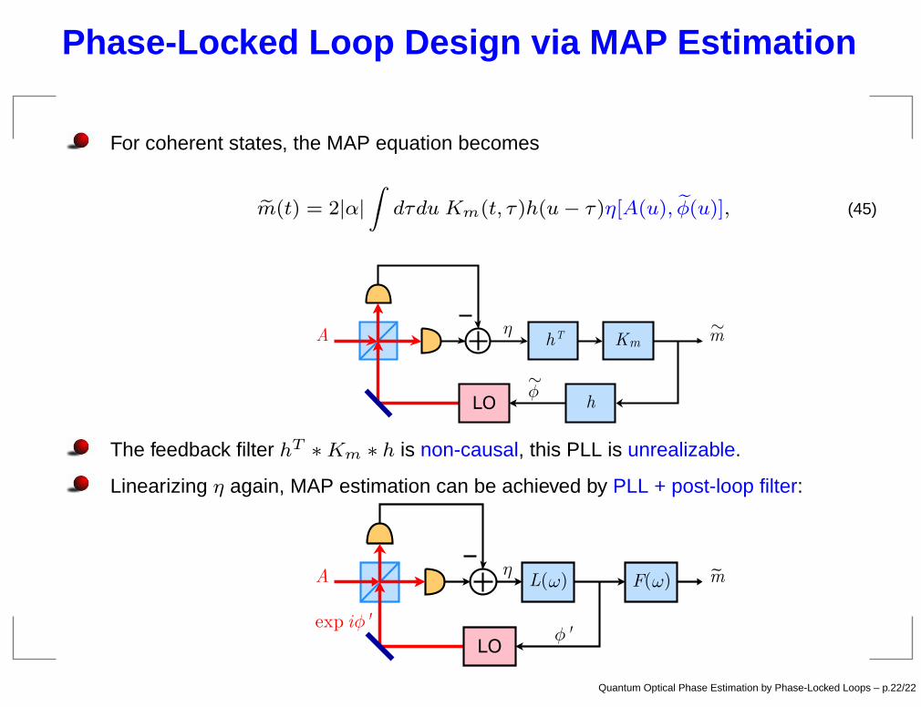
Phase-Locked Loop Design via MAP Estimation

For coherent states, the MAP equation becomes

em(t) = 2|α|Zdτdu Km(t, τ)h(u− τ)η[A(u), eφ(u)], (45)

The feedback filter hT ∗Km ∗ h is non-causal, this PLL is unrealizable.

Linearizing η again, MAP estimation can be achieved by PLL + post-loop filter:

Quantum Optical Phase Estimation by Phase-Locked Loops – p.22/22