Quantum Mechanics

Review of classical mechanics• Lagrangian L(x, x) = 1

2 mx2 −V(x), p = ∂L∂x ,

Action, S =∫

dtL, E-L equation (EOM)

0 = δS⇒ ∂t∂L∂x − ∂xL = 0

• Hamiltonian : H = xp− L,• Hamilton eq., using Poisson bracket A,B = ∂A

∂q∂B∂p −

∂A∂p

∂B∂q

q =∂H∂p = q,H , p = −∂H

∂q = p,H

Quantum Mechanics

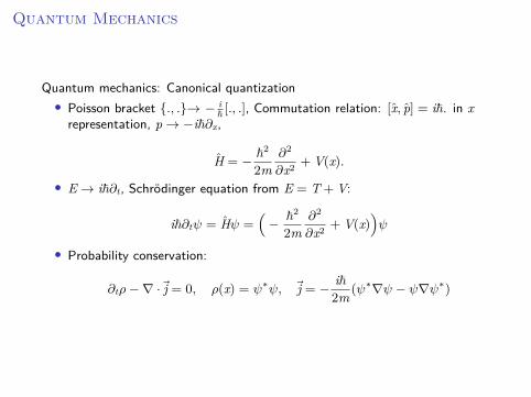
Quantum mechanics: Canonical quantization• Poisson bracket ., .→ − i

ℏ [., .], Commutation relation: [x, p] = iℏ. in xrepresentation, p→ −iℏ∂x,

H = − ℏ2

2m∂2

∂x2 + V(x).

• E→ iℏ∂t, Schrödinger equation from E = T + V:

iℏ∂tψ = Hψ =(− ℏ2

2m∂2

∂x2 + V(x))ψ

• Probability conservation:

∂tρ−∇ · j = 0, ρ(x) = ψ∗ψ, j = − iℏ2m (ψ∗∇ψ − ψ∇ψ∗)

Relativistic QM

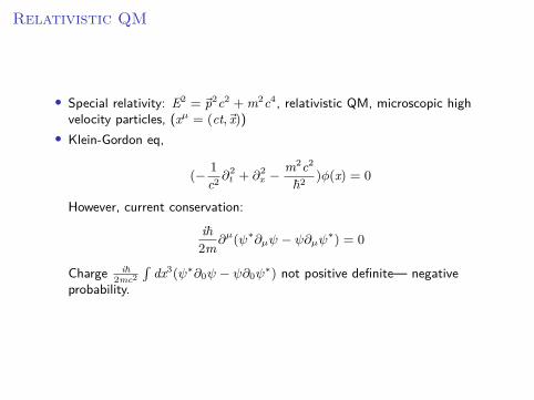
• Special relativity: E2 = p2c2 + m2c4, relativistic QM, microscopic highvelocity particles, (xµ = (ct, x))• Klein-Gordon eq,

(− 1c2 ∂

2t + ∂2

x −m2c2

ℏ2 )ϕ(x) = 0

However, current conservation:iℏ2m∂µ(ψ∗∂µψ − ψ∂µψ∗) = 0

Charge iℏ2mc2

∫dx3(ψ∗∂0ψ − ψ∂0ψ

∗) not positive definite— negativeprobability.

Relativistic QM

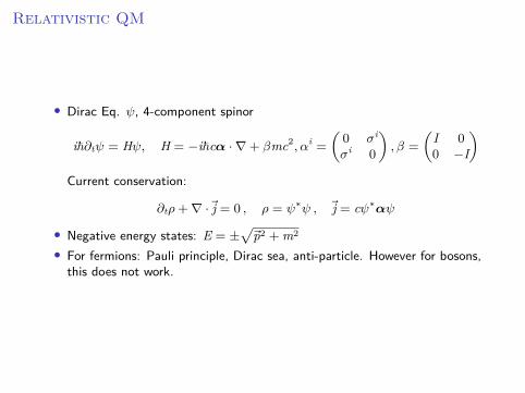
• Dirac Eq. ψ, 4-component spinor

iℏ∂tψ = Hψ, H = −iℏcα · ∇+ βmc2, αi =

(0 σi

σi 0

), β =

(I 00 −I

)Current conservation:

∂tρ+∇ · j = 0 , ρ = ψ∗ψ , j = cψ∗αψ

• Negative energy states: E = ±√

p2 + m2

• For fermions: Pauli principle, Dirac sea, anti-particle. However for bosons,this does not work.

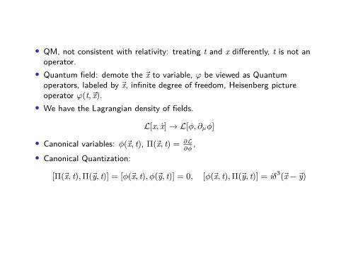
• QM, not consistent with relativity: treating t and x differently, t is not anoperator.• Quantum field: demote the x to variable, φ be viewed as Quantum

operators, labeled by x, infinite degree of freedom, Heisenberg pictureoperator φ(t, x).• We have the Lagrangian density of fields.

L[x, x]→ L[ϕ, ∂µϕ]

• Canonical variables: ϕ(x, t), Π(x, t) = ∂L∂ϕ

,• Canonical Quantization:

[Π(x, t),Π(y, t)] = [ϕ(x, t), ϕ(y, t)] = 0, [ϕ(x, t),Π(y, t)] = iδ3(x− y)

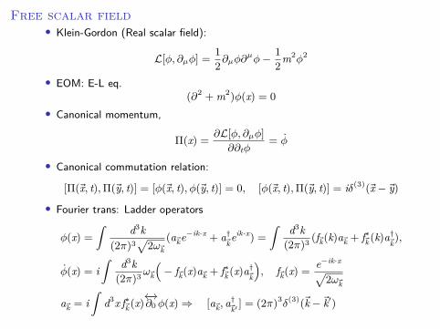
Free scalar field• Klein-Gordon (Real scalar field):

L[ϕ, ∂µϕ] =12∂µϕ∂

µϕ− 12m2ϕ2

• EOM: E-L eq.(∂2 + m2)ϕ(x) = 0

• Canonical momentum,

Π(x) = ∂L[ϕ, ∂µϕ]∂∂tϕ

= ϕ

• Canonical commutation relation:

[Π(x, t),Π(y, t)] = [ϕ(x, t), ϕ(y, t)] = 0, [ϕ(x, t),Π(y, t)] = iδ(3)(x− y)

• Fourier trans: Ladder operators

ϕ(x) =∫

d3k(2π)3

√2ωk

(ake−ik·x + a†keik·x) =

∫d3k(2π)3 (fk(k)ak + f∗k(k)a

†k),

ϕ(x) = i∫

d3k(2π)3ωk

(− fk(x)ak + f∗k(x)a

†k

), fk(x) =

e−ik·x√2ωk

ak = i∫

d3x f∗k(x)←→∂0ϕ(x)⇒ [ak, a

†k′] = (2π)3δ(3)(k− k′)

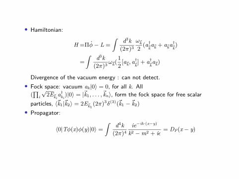
• Hamiltonian:

H =Πϕ− L =

∫d3k(2π)3

ωk2 (a†

kak + aka†

k)

=

∫d3k(2π)3ωk(

12 [ak, a

†k] + a†

kak)

Divergence of the vacuum energy : can not detect.• Fock space: vacuum ak|0⟩ = 0, for all k. All

(∏

i√

2Ekia†

ki)|0⟩ = |k1, . . . , kn⟩, form the fock space for free scalar

particles, ⟨k1 |k2⟩ = 2Ek1(2π)3δ(3)(k1 − k2)

• Propagator:

⟨0|Tϕ(x)ϕ(y)|0⟩ =∫

d4k(2π)4

ie−ik·(x−y)

k2 −m2 + iϵ = DF(x− y)

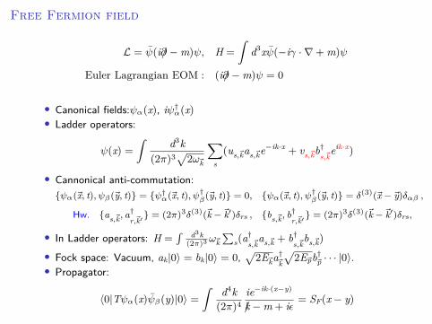
Free Fermion field

L = ψ(i∂/−m)ψ, H =

∫d3xψ(−iγ · ∇+ m)ψ

Euler Lagrangian EOM : (i∂/−m)ψ = 0

• Canonical fields:ψα(x), iψ†α(x)

• Ladder operators:

ψ(x) =∫

d3k(2π)3

√2ωk

∑s(us,kas,ke−ik·x + vs,kb†

s,keik·x)

• Cannonical anti-commutation:ψα (x, t), ψβ (y, t) = ψ†

α (x, t), ψ†β (y, t) = 0, ψα (x, t), ψ†

β (y, t) = δ(3) (x − y)δαβ ,

Hw. as,k, a†r,k′

= (2π)3δ(3) (k − k′)δrs , bs,k, b†r,k′

= (2π)3δ(3) (k − k′)δrs,

• In Ladder operators: H =∫ d3k

(2π)3ωk∑

s(a†s,k

as,k + b†s,k

bs,k)

• Fock space: Vacuum, ak|0⟩ = bk|0⟩ = 0,√

2Eka†k

√2Epb†p · · · |0⟩.

• Propagator:

⟨0|Tψα(x)ψβ(y)|0⟩ =∫

d4k(2π)4

ie−ik·(x−y)

k/−m + iϵ = SF(x− y)

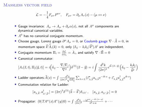
Massless vector field

L = −14FµνFµν , Fµν = ∂µAν(x)− (µ↔ ν)

• Gauge invariance: Aµ → Aµ + ∂µα(x), not all Aµ components aredynamical canonical variables.• A0 has no canonical conjugate momentum.• Choose gauge, Lorenz gauge ∂µAµ = 0, or Coulomb gauge ∇ · A = 0, in

momentum space ki Ai(k) = 0, only (δij − kikj/k2)Aj are independent.• Conjugate momentum Πi =

∂L∂Ai

= Ai, and satisfy ∇ · Π = 0• Canonical commutator:

[Ai(x, t),Πj(y, t)] = i(δij −

∇i∇j

∇2

)δ(3)(x− y) = i

∫d3k(2π)3 eik·(x−y)

(δij −

kikj

k2

)• Ladder operators:A(x) =

∫ d3k(2π)3√2Ek

∑λ=±(ε

∗λ,kaλ,ke−ik·x + ελ,ka†

λ,keik·x)

• Commutation relation for Ladder:

[aλ,k, a†λ′ ,k′

] = (2π)3δ(3)(k− k′)δλλ′ , [aλ,k, aλ′ ,k′ ] = 0

• Propagator: ⟨0|TAµ(x)Aν(y)|0⟩ =∫ d4k

(2π)4−igµνe−ik·(x−y)

k2+iϵ + · · ·

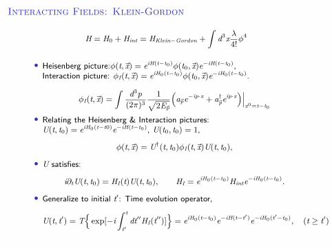
Interacting Fields: Klein-Gordon

H = H0 + Hint = HKlein−Gordon +

∫d3x λ4!ϕ

4

• Heisenberg picture:ϕ(t, x) = eiH(t−t0)ϕ(t0, x)e−iH(t−t0),Interaction picture: ϕI(t, x) = eiH0(t−t0)ϕ(t0, x)e−iH0(t−t0).

ϕI(t, x) =∫

d3p(2π)3

1√2Ep

(ape−ip·x + a†

peip·x)∣∣∣

x0=t−t0

• Relating the Heisenberg & Interaction pictures:U(t, t0) = eiH0(t−t0)e−iH(t−t0), U(t0, t0) = 1,

ϕ(t, x) = U†(t, t0)ϕI(t, x)U(t, t0),

• U satisfies:

i∂tU(t, t0) = HI(t)U(t, t0), HI = eiH0(t−t0)Hinte−iH0(t−t0).

• Generalize to initial t′: Time evolution operator,

U(t, t′) = Texp[−i

∫ t

t′dt′′HI(t′′)]

= eiH0(t−t0)e−iH(t−t′)e−iH0(t′−t0), (t ≥ t′)

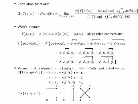
• Correlation functions:

⟨Ω|T(ϕ(x1) · · ·ϕ(xn))|Ω⟩ = limT→∞(1−iϵ)

⟨0|TϕI(x1) · · ·ϕI(xn) exp[−i∫ T−T dtHI(t)]|0⟩

⟨0|Texp[−i∫ T−T dtHI(t)]|0⟩

• Wick’s theorem:

T(ϕI(x1) · · ·ϕI(xn)) = NϕI(x1) · · ·ϕI(xn) + all possible contractions

• Vacuum matrix element: ⟨0|TϕI(x1) . . . |0⟩ = Fully contracted terms.

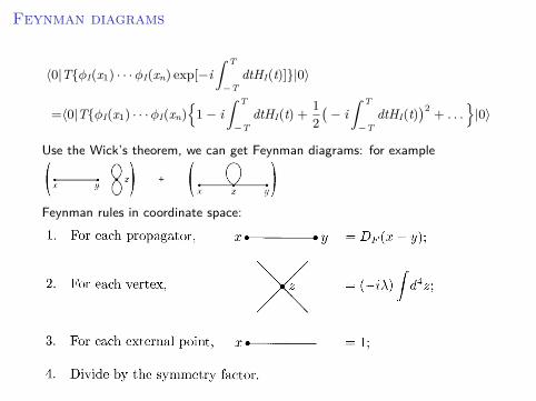
Feynman diagrams

⟨0|TϕI(x1) · · ·ϕI(xn) exp[−i∫ T

−TdtHI(t)]|0⟩

=⟨0|TϕI(x1) · · ·ϕI(xn)

1− i∫ T

−TdtHI(t) +

12(− i

∫ T

−TdtHI(t)

)2+ . . .

|0⟩

Use the Wick’s theorem, we can get Feynman diagrams: for example

Feynman rules in coordinate space:

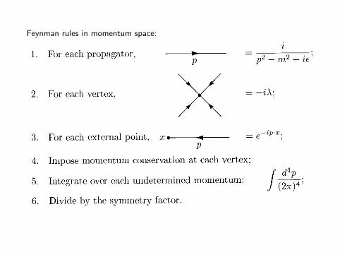
Feynman rules in momentum space:

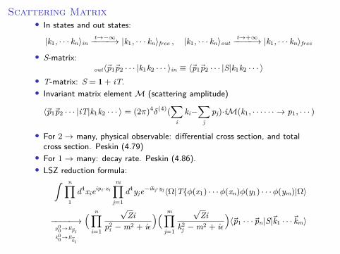
Scattering Matrix• In states and out states:

|k1, · · · kn⟩int→−∞−−−−−→ |k1, · · · kn⟩free , |k1, · · · kn⟩out

t→+∞−−−−−→ |k1, · · · kn⟩free

• S-matrix:out⟨p1p2 · · · |k1k2 · · · ⟩in ≡ ⟨p1p2 · · · |S|k1k2 · · · ⟩

• T-matrix: S = 1 + iT.• Invariant matrix element M (scattering amplitude)

⟨p1p2 · · · |iT|k1k2 · · · ⟩ = (2π)4δ(4)(∑

iki−

∑j

pj)·iM(k1, · · · · · · → p1, · · · )

• For 2→ many, physical observable: differential cross section, and totalcross section. Peskin (4.79)• For 1→ many: decay rate. Peskin (4.86).• LSZ reduction formula:∫ n∏

1d4xieipi·xi

m∏j=1

d4yje−ikj·yj⟨Ω|Tϕ(x1) · · ·ϕ(xn)ϕ(y1) · · ·ϕ(ym)|Ω⟩

−−−−−→p0

0→Epik00→Eki

( n∏i=1

√Zi

p2i −m2 + iϵ

)( m∏j=1

√Zi

k2j −m2 + iϵ

)⟨p1 · · · pn|S|k1 · · · km⟩

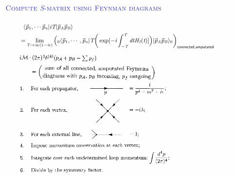
Compute S-matrix using Feynman diagrams

⟨p1, · · · pn|iT|pApB⟩

= limT→∞(1−iϵ)

(0⟨p1, · · · , pn|T

(exp[−i

∫ T

−TdtHI(t)]

)|pApB⟩0

)connected,amputated

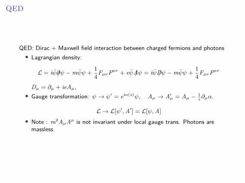
QED

QED: Dirac + Maxwell field interaction between charged fermions and photons• Lagrangian density:

L = iψ∂/ψ −mψψ +14FµνFµν + eψA/ψ = iψD/ψ −mψψ +

14FµνFµν

Dµ = ∂µ + ieAµ,• Gauge transformation: ψ → ψ′ = eiα(x)ψ, Aµ → A′

µ = Aµ − 1e∂µα.

L → L[ψ′,A′] = L[ψ,A]

• Note : m2AµAµ is not invariant under local gauge trans. Photons aremassless.

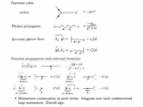
Feynman rules:

Fermion propagators and external fermions:

• Momentum conservation at each vertex. Integrate over each undeterminedloop momentum. Overall sign.

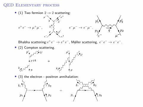
QED Elementary process• (1) Two fermion 2→ 2 scattering:

e+e− → µ+µ−, e−µ− → e−µ−.

Bhabha scattering:e+e− → e+e−, Mo/ller scattering, e−e− → e−e−.• (2) Compton scattering.

• (3) the electron - positron annihalation:

QFTII

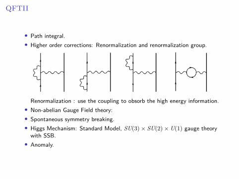
• Path integral.• Higher order corrections: Renormalization and renormalization group.

Renormalization : use the coupling to obsorb the high energy information.• Non-abelian Gauge Field theory:• Spontaneous symmetry breaking.• Higgs Mechanism: Standard Model, SU(3)× SU(2)×U(1) gauge theory

with SSB.• Anomaly.