∆ελτίο της Ελληνικής Γεωλογικής Εταιρίας τοµ. XXXVII, 2007 Πρακτικά 11ου ∆ιεθνούς Συνεδρίου, Αθήνα, Μάιος 2007

Bulletin of the Geological Society of Greece vol. XXXVII, 2007 Proceedings of the 11th International Congress, Athens, May, 2007

QUANTITATIVE FAULT ANALYSIS AT ARKITSA, CENTRAL GREECE, USING TERRESTRIAL LASER-SCANNING

(“LIDAR”)

Kokkalas S.*1, Jones R. R.2, 3, McCaffrey K. J. W.4, and Clegg P.4

1 University of Patras, Department of Geology, Laboratory of Structural Geology, 26500 Patras,

Greece, skokalas@upatras.gr 2 Geospatial Research Ltd., University of Durham, DH1 3LE, UK,

richard@geospatial-research.com 3 e-Science Research Institute, University of Durham, DH1 3LE, UK.

4 Department of Earth Sciences,

University of Durham, DH1 3LE, UK, k.j.w.mccaffrey@durham.ac.uk, p.clegg@durham.ac.uk

Abstract

We applied terrestrial laser scanning (ground-based LiDAR) in the Arkitsa fault zone, an area of active extension along the North Evia Gulf in Central Greece. The study area includes well exposed fault surfaces with large accumulated slip and this allowed detailed measurements of the geometry of the fault planes to be acquired. Laser-scan data enable ultra high-resolution three-dimensional digital terrain models of the recently exposed active fault to be created, in order to apply quantitative fault and slip-vector analysis. This study demonstrates the way in which the Arkitsa Fault is segmented on a smaller scale. The variation in dip and strike across individual fault panels is quantified, and shows the extent to which the fault panel surfaces are non-planar. Although the dip of the different fault panels varies considerably, the average orientation of the slip-vectors on the panels are approximately coincident. The fault is steeply oblique sinistral-normal, with average displacement vector plunging 55° towards 340°.

Key words: fault segmentation, digital scanning, slip-vectors, fault scarp, Evoikos Gulf, Central Greece.

1. Introduction In recent years the increasing development of new digital acquisition techniques, such as digital photography, ground penetrating radar and terrestrial laser scanning (TLS) has provided powerful tools for field documentation and investigation in geosciences (e.g. McCaffrey et al., 2005). The appearance of TLS (also known as ground-based LiDAR) has provided a new data source of geometric information in earth science research. The core technology of TLS is a ground based device that uses a laser to measure automatically the three-dimensional coordinates of a given region of the surface of an object, in a systematic order at a high rate in (near) real time (from Boehler and Marbs, 2002). In recent years, petroleum geologists have developed sophisticated methods using high resolution 3D reflection seismic survey data to build detailed 3D models of sub-surface geological architectures for use in hydrocarbon exploration and production. Modern optical 3D measurement and visualisation techniques now make it possible to analyse rock

2

outcrops exposed at the surface using an approach that is conceptually comparable to that used in petroleum exploration.

Tripod-mounted laser scanners have a great variety of range accuracies (1 to 50 mm) and target distances (up to 2000 m) from the sensor, depending on the exact specification of the equipment used. The main advantages of the laser scanner are that it can typically achieve accuracies of 5 mm or better at a 200 m range, and that acquisition of outcrop surface topography is relatively rapid (typically just a few minutes). The main disadvantages are the high cost of TLS equipment (€30k-€150k), and that analysis of the data can be very time consuming.

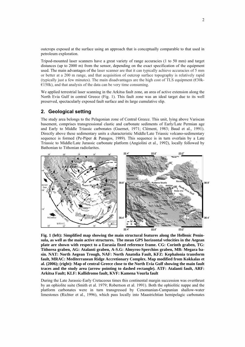
We applied terrestrial laser scanning in the Arkitsa fault zone, an area of active extension along the North Evia Gulf in central Greece (Fig. 1). This fault zone was an ideal target due to its well preserved, spectacularly exposed fault surface and its large cumulative slip.

2. Geological setting The study area belongs to the Pelagonian zone of Central Greece. This unit, lying above Variscan basement, comprises transgressional clastic and carbonate sediments of Early/Late Permian age and Early to Middle Triassic carbonates (Guernet, 1971; Clément, 1983; Baud et al., 1991). Directly above these sedimentary units a characteristic Middle/Late Triassic volcano-sedimentary sequence is formed (Pe-Piper & Panagos, 1989). This sequence is in turn overlain by a Late Triassic to Middle/Late Jurassic carbonate platform (Angiolini et al., 1992), locally followed by Bathonian to Tithonian radiolarites.

Fig. 1 (left): Simplified map showing the main structural features along the Hellenic Penin-sula, as well as the main active structures. The mean GPS horizontal velocities in the Aegean plate are shown with respect to a Eurasia fixed reference frame. CG: Corinth graben, TG: Tithorea graben, AG: Atalanti graben, A-S.G: Almyros-Sperchios graben, MB: Megara ba-sin. NAT: North Aegean Trough, NAF: North Anatolia Fault, KFZ: Kephalonia transform fault, MRAC: Mediterranean Ridge Accretionary Complex. Map modified from Kokkalas et al. (2006); (right): Map of central Greece close to the North Evia Gulf showing the main fault traces and the study area (arrow pointing to dashed rectangle). ATF: Atalanti fault, ARF: Arkitsa Fault; KLF: Kallidromo fault, KVF: Kamena Vourla fault

During the Late Jurassic-Early Cretaceous times this continental margin succession was overthrust by an ophiolite suite (Smith et al. 1979; Robertson et al. 1991). Both the ophiolitic nappe and the platform carbonates were in turn transgressed by Cenomanian-Campanian shallow-water limestones (Richter et al., 1996), which pass locally into Maastrichtian hemipelagic carbonates

3

(Katsikatsos et al., 1986). Finally, carbonate sedimentation terminated with flysch deposition Paleocene-Eocene (Ypresian) age (Richter et al., 1996).

Since the Upper Miocene to present, the area of Central Greece has been affected by ongoing active crustal extension in a NNE-SSW direction, mainly by two major mechanisms: the westward motion of the Anatolia plate, and the slab retreat (roll-back) of the African slab under the Hellenic Peninsula (Meijer and Wortel 1997; Doutsos and Kokkalas 2001). The central part of the Hellenic Peninsula represents the classic “basin-and-range”-type extensional area in Greece. Most of the extensional strain is accommodated by four WNW-trending grabens: the Corinth, Tithorea, Atalanti and Almyros-Sperchios graben (Westaway, 1991; Fig. 1 left). Most of these are asymmetric, with N-dipping master faults, which are usually segmented along their strike (Doutsos and Poulimenos 1992; Roberts and Koukouvelas 1996; Kokkalas et al. 2006).

The age of the synrift deposits along this WNW-ESE fault direction ranges from Late Miocene-Early Pliocene in the east (i.e. Megara basin) to Pleistocene in the west (i.e. Sperchios graben or the west part of Corinth graben), showing the westward propagation of the rift zones, probably due to accelerated extensional deformation during the Late Pliocene (Doutsos and Kokkalas, 2001 and references therein). The Arkitsa fault, which is the case example of this study, is a part of the segmented north-dipping fault system of Sperchios-Kamena Vourla, lying along the south coast of North Evia Gulf (Figs. 1 and 2). This structure has a length of almost 100 km. The footwall of the Arkitsa and Kamena Vourla fault consists of Late Triassic to Middle/Late Jurassic platform carbonates, while the hangingwall consists of Lower Pliocene-Pleistocene to Quaternary sediments. The vertical offset varies significantly along strike and for the Arkitsa segment a minimum offset on the order of 500 m can be estimated. Another significant active fault zone is located south of this fault zone, the Atalanti fault zone which is also segmented in 4-5 prominent segments (Pavlides et al. 2004).

Historical seismic catalogues in the Gulf of Evia area contain records of around thirteen rupture events from 426 BC up to the last destructive Atalanti event in 1894 AD (Ganas et al. 1998, 2006), although there is much uncertainty both in epicentre location and earthquake magnitude (Ambraseys and Jackson, 1990).

The geometry of a fault, which is often oversimplified in most fault models or earthquake simula-tions over a large range of scales, provides fundamental control on its mechanical behaviour and reflects the processes by which the fault grew. Existing failure criteria for rocks typically assume that fractures are planar, although field observations of naturally occurring fracture systems show that individual surfaces are often observed to be significantly non-planar. This can reflect how they are affected during slip by the mechanical heterogeneities inherited in the surrounding rock. More-over striations on a fault plane can show substantial deviations during single earthquakes because of changes of slip with time during the rupture propagation. It is not common to have access to such well preserved exhumed fault surfaces with a large accumulated slip as in our study area. Therefore, this paper aims to shed some light to the 3D geometry of well exposed fracture surfaces and the slip distribution on them, in a detail that couldn’t be achieved before.

3. Methods 3.1. General In previous studies, LiDAR has proven useful in engineering geologic applications (Pack, 2002) and for the monitoring of ground movements (Kayen et al, 2004; Bawden et al. 2004). LiDAR systems have also been applied to landslides in Europe (Paar et al, 2000; Scheikl et al., 2000; Rowlands et al. 2003), and in the U.S. (Collins and Sitar, 2004). It is also becoming more common for geologists to utilise digital survey technologies (e.g. Ahlgren et al. 2002; Jones et al. 2004;

4

Bellian et al. 2005; McCaffrey et al. 2005) where data are captured in a digital format using GPS and TLS, and viewed using a GIS or geoscientific visualisation software.

The TLS technique can be applied to a broad range of geological problems, including: • Quantitative 3D models for use in geotechnical surveys and slope stability analysis; • The provision of sub-seismic scale rock structure analogues for modelling permeability

and fluid flow in hydrocarbon reservoirs; • Rapid collection of post-earthquake failure geometries of ground and structures prior to

modification by post disaster recovery efforts and natural processes; • As a tool for the training and teaching of students and professional geo-scientists in the

complex geometry of structures and sedimentary systems (e.g. McCaffrey et al. 2003) • Providing access to geological outcrops located in inaccessible or dangerous areas.

The LiDAR technology is a natural extension of laser-rangefinder systems or electronic distance meters (EDMs) used commonly in survey applications. With this technology, a laser beam scans sequentially in all directions to measure the precise distance of objects across the scene. The laser repeatedly shoots out a pulse of light at each rotation point of the scanner. The pulse hits the object and scatters a portion of the light back. As the scanning laser shots bounce off objects at various distances from the scanner, point measurements are collected that define the object’s shape. By timing the round trip of each laser pulse, the range is determined for each scanned point, and the point’s geospatial coordinates are recorded relative to the scanner. By knowing the position and orientation of the instrument, each point in the acquired dataset (referred to as a “point cloud”), can be transformed to XYZ coordinates in a global coordinate system. Point clouds may also include intensity and colour information. In our case, the end result is a cloud of points whose three-dimensional coordinates correspond to the points on the fault surface with a regular angular spacing (Figs. 3 and 4). In some cases we can have data voids (“data shadows”), which are sections within the point cloud, more than twice the point density of the scan in size, containing no data.

For this study we used a Riegl LMS Z420i laser-scanner, together with a Nikon D70 digital camera mounted on top to photograph the area scanned. According to the manufacturers specifications, this type of scanner has a maximum angular acuity of 0.003° in both horizontal and vertical directions, and a longitudinal precision of ±25mm or better. A laptop is used in the field to control the scanner and the camera, as well as for data storage and quality control of data gathering during the acquisition process. A single scan can sweep up to 360° horizontally and up to ±40° vertically. The scanner makes millions of individual x, y, z position measurements, at a rate of 8,000 to 12,000 points/second. A low resolution scan would typically capture 1 to 4 million points over a 360° area, while a very high resolution scan will capture tens (or even hundreds) of millions of points from a single fault panel. The time required for an individual scan with a reasonably high sample density of points per setup (e.g. 10 million targeted points) is typically less than 15 minutes. Point measurements at a coarser density (e.g. 1 million target points) take around 1 minute. Several scan stations are chosen along the target outcrop to allow it to be scanned from a number of different angles, with a large degree of overlap between adjacent scans. This helps to minimise the amount of data shadows in the resultant model. Following acquisition, the individual scans are geo-referenced and merged to form a single virtual outcrop model.

5

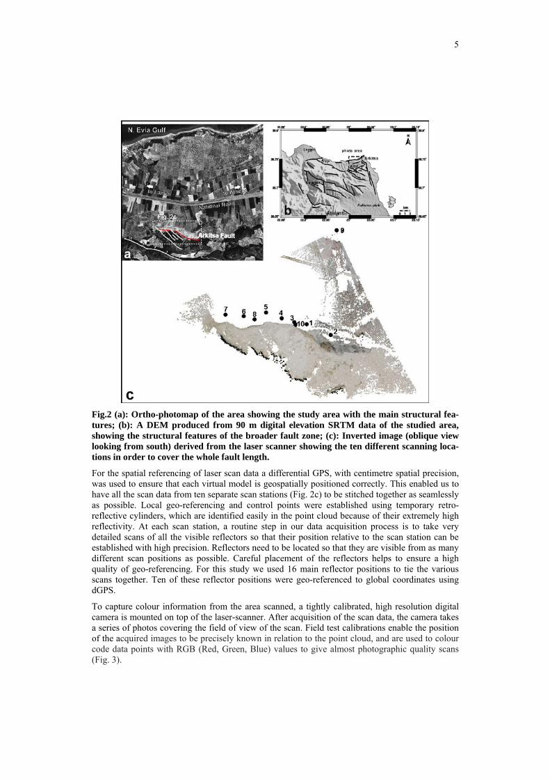
Fig.2 (a): Ortho-photomap of the area showing the study area with the main structural fea-tures; (b): A DEM produced from 90 m digital elevation SRTM data of the studied area, showing the structural features of the broader fault zone; (c): Inverted image (oblique view looking from south) derived from the laser scanner showing the ten different scanning loca-tions in order to cover the whole fault length.

For the spatial referencing of laser scan data a differential GPS, with centimetre spatial precision, was used to ensure that each virtual model is geospatially positioned correctly. This enabled us to have all the scan data from ten separate scan stations (Fig. 2c) to be stitched together as seamlessly as possible. Local geo-referencing and control points were established using temporary retro-reflective cylinders, which are identified easily in the point cloud because of their extremely high reflectivity. At each scan station, a routine step in our data acquisition process is to take very detailed scans of all the visible reflectors so that their position relative to the scan station can be established with high precision. Reflectors need to be located so that they are visible from as many different scan positions as possible. Careful placement of the reflectors helps to ensure a high quality of geo-referencing. For this study we used 16 main reflector positions to tie the various scans together. Ten of these reflector positions were geo-referenced to global coordinates using dGPS.

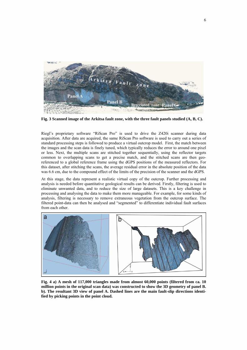
To capture colour information from the area scanned, a tightly calibrated, high resolution digital camera is mounted on top of the laser-scanner. After acquisition of the scan data, the camera takes a series of photos covering the field of view of the scan. Field test calibrations enable the position of the acquired images to be precisely known in relation to the point cloud, and are used to colour code data points with RGB (Red, Green, Blue) values to give almost photographic quality scans (Fig. 3).

6

Fig. 3 Scanned image of the Arkitsa fault zone, with the three fault panels studied (A, B, C).

Riegl’s proprietary software “RiScan Pro” is used to drive the Z420i scanner during data acquisition. After data are acquired, the same RiScan Pro software is used to carry out a series of standard processing steps is followed to produce a virtual outcrop model. First, the match between the images and the scan data is finely tuned, which typically reduces the error to around one pixel or less. Next, the multiple scans are stitched together sequentially, using the reflector targets common to overlapping scans to get a precise match, and the stitched scans are then geo-referenced to a global reference frame using the dGPS positions of the measured reflectors. For this dataset, after stitching the scans, the average residual error in the absolute position of the data was 6.6 cm, due to the compound effect of the limits of the precision of the scanner and the dGPS.

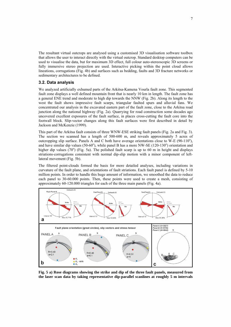
At this stage, the data represent a realistic virtual copy of the outcrop. Further processing and analysis is needed before quantitative geological results can be derived. Firstly, filtering is used to eliminate unwanted data, and to reduce the size of large datasets. This is a key challenge in processing and analysing the data to make them more manageable. For example, for some kinds of analysis, filtering is necessary to remove extraneous vegetation from the outcrop surface. The filtered point-data can then be analysed and “segmented” to differentiate individual fault surfaces from each other.

Fig. 4 a) A mesh of 117,000 triangles made from almost 60,000 points (filtered from ca. 10 million points in the original scan data) was constructed to show the 3D geometry of panel B. b). The resultant 3D view of panel A. Dashed lines are the main fault-slip directions identi-fied by picking points in the point cloud.

7

The resultant virtual outcrops are analysed using a customised 3D visualisation software toolbox that allows the user to interact directly with the virtual outcrop. Standard desktop computers can be used to visualise the data, but for maximum 3D effect, full colour auto-stereoscopic 3D screens or fully immersive stereo projection are used. Interactive picking within the point cloud allows lineations, corrugations (Fig. 4b) and surfaces such as bedding, faults and 3D fracture networks or sedimentary architectures to be defined.

3.2. Data analysis We analyzed artificially exhumed parts of the Arkitsa-Kamena Vourla fault zone. This segmented fault zone displays a well defined mountain front that is nearly 10 km in length. The fault zone has a general ENE trend and moderate to high dip towards the NNW (Fig. 2b). Along its length to the west the fault shows impressive fault scarps, triangular faulted spurs and alluvial fans. We concentrated our analysis in the excavated eastern part of the fault zone, close to the Arkitsa road junction along the national highway (Fig. 2a). Quarrying for road construction some decades ago uncovered excellent exposures of the fault surface, in places cross-cutting the fault core into the footwall block. Slip-vector changes along this fault surfaces were first described in detail by Jackson and McKenzie (1999).

This part of the Arkitsa fault consists of three WNW-ESE striking fault panels (Fig. 2a and Fig. 3). The section we scanned has a length of 500-600 m, and reveals approximately 5 acres of outcropping slip surface. Panels A and C both have average orientations close to W-E (90-110o), and have similar dip values (50-60o), while panel B has a more NW-SE (120-130o) orientation and higher dip values (70o) (Fig. 5a). The polished fault scarp is up to 60 m in height and displays striations-corrugations consistent with normal dip-slip motion with a minor component of left-lateral movement (Fig. 5b).

The filtered point-clouds formed the basis for more detailed analyses, including variations in curvature of the fault plane, and orientations of fault striations. Each fault panel is defined by 5-10 million points. In order to handle this huge amount of information, we smoothed the data to reduce each panel to 30-60.000 points. Then, these points were used to create a mesh, consisting of approximately 60-120.000 triangles for each of the three main panels (Fig. 4a).

Fig. 5 a) Rose diagrams showing the strike and dip of the three fault panels, measured from the laser scan data by taking representative dip-parallel scanlines at roughly 5 m intervals

8

along the fault panels. Manual measurements from the lower parts of the fault panels were also added using a compass/clinometer on the outcrop. b) Stereonets showing slickenline slip vectors measured from the laser-scan point cloud, together with the three principal stress axes, strain ratio R and the slip deviation parameter [a]. c) Stereonet displaying the variation in 3D orientation of the three fault panels, shown by plotting the vector normals for a ran-dom sub-set of triangles from the meshed laser-scan data for each panel. Contouring of vec-tor normals include almost 5700-6000 points, in each panel.

Once the data is meshed, a vector normal can be derived for each triangle in the mesh, equivalent to the pole to the fault plane at that point. The plot of vector normals gives a view of the variation in 3D orientation of each fault panel. (Fig. 5c).

One of the most spectacular and characteristic indicators of fault displacement are the corrugations on the slip plane. The corrugations are characterized by sinusoidal profiles normal to their long axes , displaying ridges and grooves, and less commonly they show culminations and depressions along their axes, indicative of the irregular shape of the curved fault surface (Fig. 6b). There are many ways to form these kind of irregularities on a faulted surface. Linkage of precursory faults could generate corrugations on the fault surface or they might be caused due to spatial variations in strength of the fault zone. Irrespective of the underlying cause of the corrugations, it seems that those corrugations parallel to the recent slip direction are the most stable and have the potential to be amplified or better preserved.

Three main zones can be distinguished in an orthogonal section through the fault scarps: a damage host rock area in the footwall block, a gouge-cataclasis zone representing the localization of deformation, which progressively grades to more extreme localization of deformation with formation of thin cement-dominated horizons and thin re-cemented hangingwall breccia sheets (Fig. 6a). In the exhumed part of the fault surface one might expect to find evidence of all the slip vector orientations from successive faulting episodes, however they are often overprinted by the most recent slip events. In places under the thin cemented sheets, we observed areas with a different set of slip lineations, which are mainly marked on clay layers, often foliated parallel to the fault surface. Also some irregular U-shaped centimetre-scale markings have been observed on the fault surface, which are well preserved beneath a layer of brecciated material. These markings may possibly be related to either hangingwall block rotation during shear deformation along the slip surface or may represent tool-tracks caused by resistant colluvial clasts scratching the contact surface (Jackson and McKenzie, 1999). Thus, it is quite difficult to define accurately older reactivation events along the whole surface.

Numerous fractures cut the fault surface; some are strike-parallel, others are oblique to the dip direction (Fig. 6a and 7a). Fractures include some synthetic hybrid fractures, tension gashes, as well as comb fractures which are almost perpendicular to the slip plane. Some of them displace the fault surface with a thrust sense of offset. Jackson and McKenzie (1999) argued that these structures may have formed as a result of the rock relaxation after the excavation of the hangingwall material. In the steeply dipping fault panel B, it appears that fractures increase in density and vary in orientation and possibly represent breaching of the panel by numerous small splays, as well as interaction with the large fault panels A and C.

9

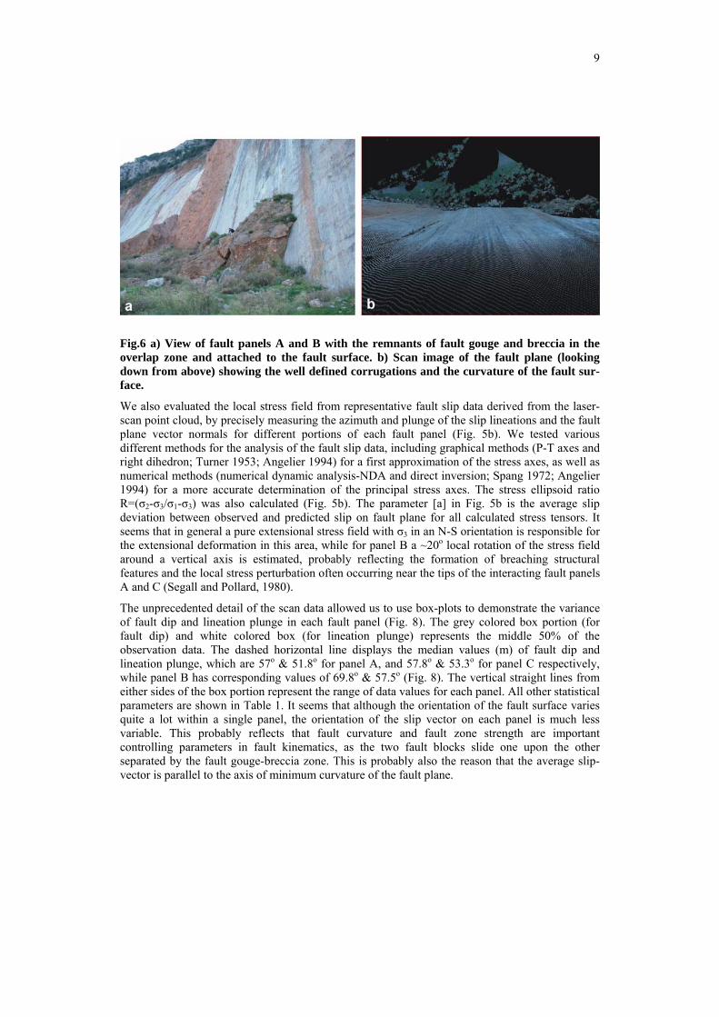
Fig.6 a) View of fault panels A and B with the remnants of fault gouge and breccia in the overlap zone and attached to the fault surface. b) Scan image of the fault plane (looking down from above) showing the well defined corrugations and the curvature of the fault sur-face.

We also evaluated the local stress field from representative fault slip data derived from the laser-scan point cloud, by precisely measuring the azimuth and plunge of the slip lineations and the fault plane vector normals for different portions of each fault panel (Fig. 5b). We tested various different methods for the analysis of the fault slip data, including graphical methods (P-T axes and right dihedron; Turner 1953; Angelier 1994) for a first approximation of the stress axes, as well as numerical methods (numerical dynamic analysis-NDA and direct inversion; Spang 1972; Angelier 1994) for a more accurate determination of the principal stress axes. The stress ellipsoid ratio R=(σ2-σ3/σ1-σ3) was also calculated (Fig. 5b). The parameter [a] in Fig. 5b is the average slip deviation between observed and predicted slip on fault plane for all calculated stress tensors. It seems that in general a pure extensional stress field with σ3 in an N-S orientation is responsible for the extensional deformation in this area, while for panel B a ~20o local rotation of the stress field around a vertical axis is estimated, probably reflecting the formation of breaching structural features and the local stress perturbation often occurring near the tips of the interacting fault panels A and C (Segall and Pollard, 1980).

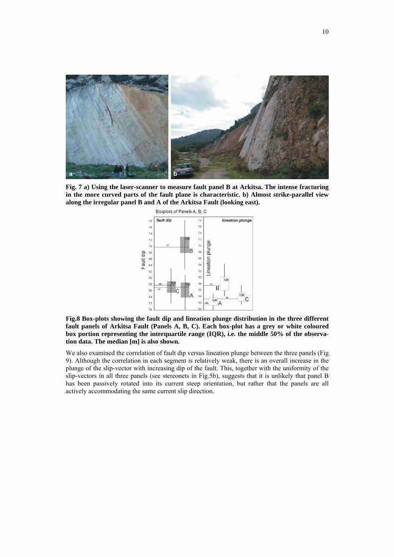
The unprecedented detail of the scan data allowed us to use box-plots to demonstrate the variance of fault dip and lineation plunge in each fault panel (Fig. 8). The grey colored box portion (for fault dip) and white colored box (for lineation plunge) represents the middle 50% of the observation data. The dashed horizontal line displays the median values (m) of fault dip and lineation plunge, which are 57o & 51.8o for panel A, and 57.8o & 53.3o for panel C respectively, while panel B has corresponding values of 69.8o & 57.5o (Fig. 8). The vertical straight lines from either sides of the box portion represent the range of data values for each panel. All other statistical parameters are shown in Table 1. It seems that although the orientation of the fault surface varies quite a lot within a single panel, the orientation of the slip vector on each panel is much less variable. This probably reflects that fault curvature and fault zone strength are important controlling parameters in fault kinematics, as the two fault blocks slide one upon the other separated by the fault gouge-breccia zone. This is probably also the reason that the average slip-vector is parallel to the axis of minimum curvature of the fault plane.

10

Fig. 7 a) Using the laser-scanner to measure fault panel B at Arkitsa. The intense fracturing in the more curved parts of the fault plane is characteristic. b) Almost strike-parallel view along the irregular panel B and A of the Arkitsa Fault (looking east).

Fig.8 Box-plots showing the fault dip and lineation plunge distribution in the three different fault panels of Arkitsa Fault (Panels A, B, C). Each box-plot has a grey or white coloured box portion representing the interquartile range (IQR), i.e. the middle 50% of the observa-tion data. The median [m] is also shown.

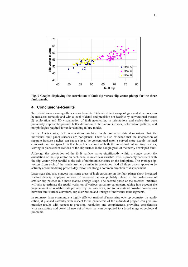
We also examined the correlation of fault dip versus lineation plunge between the three panels (Fig. 9). Although the correlation in each segment is relatively weak, there is an overall increase in the plunge of the slip-vector with increasing dip of the fault. This, together with the uniformity of the slip-vectors in all three panels (see stereonets in Fig.5b), suggests that it is unlikely that panel B has been passively rotated into its current steep orientation, but rather that the panels are all actively accommodating the same current slip direction.

11

40

45

50

55

60

65

70

45 50 55 60 65 70 75 80fault dip

slip

-vec

tor p

lung

e

Panel APanel BPanel C

Fig. 9 Graphs displaying the correlation of fault dip versus slip vector plunge for the three fault panels.

4. Conclusions-Results Terrestrial laser-scanning offers several benefits: 1) detailed fault morphologies and structures, can be measured remotely and with a level of detail and precision not feasible by conventional means; 2) exploration and 3D visualization of fault geometries, in orientations and scales that were previously impossible, provide better definition of the failure surfaces, deformation patterns, and morphologies required for understanding failure modes.

In the Arkitsa area, field observations combined with laser-scan data demonstrate that the individual fault panel surfaces are non-planar. There is also evidence that the intersection of separate fracture patches can cause slip to be concentrated upon a curved more steeply inclined composite surface (panel B) that breaches sections of both the individual intersecting patches, leaving in places relict sections of the slip surface in the hangingwall of the newly developed fault.

Although the orientation of the fault surface varies significantly within a single panel, the orientation of the slip vector on each panel is much less variable. This is probably consistent with the slip-vector lying parallel to the axis of minimum curvature on the fault plane. The average slip-vectors from each of the panels are very similar in orientation, and all three panels appear to be actively accommodating present-day tectonism along a common direction of displacement.

Laser-scan data also suggest that some areas of high curvature on the fault planes show increased fracture density, implying an area of increased damage probably related to the coalescence of smaller slip patches in a more mature linkage stage. The second phase of the research initiative will aim to estimate the spatial variation of various curvature parameters, taking into account the huge amount of available data provided by the laser scan, and to understand possible correlations between fault surface curvature, slip distribution and linkage of individual fault segments.

In summary, laser scanning is a highly efficient method of measuring outcrop geometry. Its appli-cation, if planned carefully with respect to the parameters of the individual project, can give im-pressive results with respect to precision, resolution and completeness, providing geoscientists with an exciting and powerful new set of tools that can be applied to a broad range of geological problems.

12

Table 1 Mean SE Mean St. Deviation Variance Coef. Var Fault PanelA Fault dip 56,39 0,48 2,88 8,33 5,12 Lineation plunge 51,63 0,38 2,27 5,17 4,41 Fault Panel B Fault dip 70,26 0,50 3,65 13,31 5,19 Lineation plunge 58,17 0,35 2,56 6,54 4,40 Fault Panel C Fault dip 57,30 0,49 2,85 8,17 4,98 Lineation plunge 53,84 0,28 1,62 2,65 3,02

5. Acknowledgments S.K would like to thank the Rock Fracture Project at Stanford University which hosted him during the preparation of this work. Tim Wright is thanked for help during fieldwork.

6. References Ahlgren, S., Holmlund, J. 2002. Outcrop Scans Give New View. American Association of Petro-

leum Geologists Explorer, July 2002. Available online at: http://www.aapg.org/ex-plorer/geophysical_corner/2002/07gpc.cfm.

Ambraseys, N.N., Jackson, J.A., 1990. Seismicity and associated strain of central Greece between 1890 and 1988. Geophysical Journal International 101, 663-708.

Angelier, J., 1994. Fault slip analysis and paleostress reconstruction. In: Hancock, P.L. (Ed.), Con-tinental Deformation. Pergamon Press, Oxford, pp. 53-100.

Angiolini, L., Dragonetti, L., Muttoni, G. & Nicora,A. 1992. Triassic stratigraphy in the island of Idra (Greece). Riv. It. Paleont. Strat. 98/2, 137-180.

Baud, A., Jenny, C., Papanikolaou, D., Sideris, C. &Stampfli, G.M. 1991. New observations on Permian stratigraphy in Greece and geodynamic implication. Bull. Geol. Soc. Greece XXV/1, 187-206.

Bawden, G. W., Kayen, R., Silver, M. H., Brandt, J. T., and Collins, B. D., 2004. Evaluating tripod LIDAR as an earthquake response tool, EOS Trans. Am. Geophys. Union, 85, 47, Fall Meeting Supplement, Abstract S51C-0170R.S.

Bellian, J.A., Kerans, C., Jennette, D.C. 2005. Digital outcrop models: applications of terrestrial scanning lidar technology in stratigraphic modelling. Journal of Sedimentary Research 75, 166-176.

Boehler, M. and Marbs A., 2002 3D scanning instruments.Proceedings, International Workshop on Scanning for Cultural Heritage Recording, Corfu, Greece. 160 pages: 9-12.

Clement, B. 1983. Évolution géodynamique d’un secteur des Hellénides: l’Attique septentrionale. Annales Société géologique du Nord, 101, 87–96.

Collins, B. D., and Sitar, N., 2004. Application of high-resolution 3-D laser scanning to slope sta-bility studies, 39th Annual Symposium on Engineering Geology and Geotechnical Engi-neering,Butte, Mont.

Doutsos, T., Kokkalas S. 2001. Stress and deformation in the Aegean region. Journal of Structural Geology 23, 455-472.

Doutsos, T., Poulimenos, G., 1992. Geometry and kinematics of active faults and their seismotec-tonic significance in the western Corinth-Patras rift (Greece). Journal of Structural Geology 14, 689-699.

Ganas, A., Roberts, G., Memou, P., 1998. Segment boundaries, the 1894 ruptures and strain patterns along the Atalanti fault, central Greece. Journal of Geodynamics, 26, 461-486.

13

Ganas, A., Sokos, E., Agalos, A., Leontakianakos, G., Pavlides, S., 2006. Coulomb stress triggering of earthquakes along the Atalanti fault, Central Greece: Two April 1894 M6+ events and stress changes patterns. Tectonophysics, 420, 357-369.

Guernet, C., 1971. Etudes géologiques en Eubée et dans les régions voisines (Grèc). Thèse d’Etat Univ. Paris, 395 pp., Paris.

Jackson, J., McKenzie, D., 1999. A hectare of fresh striations on the Arkitsa fault, central Greece. Journal of Structural Geology, 21, 1-6.

Jones, R.R., McCaffrey, K.J.W, Wilson, R.W. & Holdsworth, R.E. 2004. Digital field data acqui-sition towards increased quantification of uncertainty during geological mapping. In: Cur-tis, A. & Wood, R.(eds.) Geological Prior Information. Geological Society Special Publica-tion 239, In Press

Katsikatsos, G., Migiros, G.P., Triantaphyllis, M. & Mettos, A. 1986: Geological structure of in-ternal Hellenides (E. Thessaly-SW. Macedonia, Euboea-Attica-Northern Cyclades Islands and Lesvos). In: Papastamatiou J. memorial issue (Ed. I.G.M.E). Special Issue, Geological and Geophysical Research, Athens, 191-212.

Kayen, R., Barnhardt, W., Carkin, B., Collins, B. D., Grossman, E. E., Minasian, D., Thompson, E., 2004. Imaging the M 7.9 Denali Fault earthquake 2002 rupture at the Delta River using LIDAR, RADAR, and SASW surface wave geophysics, EOS Trans. Am. Geophys. Union, 85 (47), Fall Meeting Supplement, Abstract S11A-0999.

Kokkalas, S., Xypolias, P., Koukouvelas, I., and Doutsos, T. (2006) Postcollisional contractional and extensional deformation in the Aegean region, in Dilek, Y., and Pavlides, S., eds., Postcollisional tectonics and magmatism in the Mediterranean region and Asia: Geological Society of America Special Paper 409, p. 97–123, doi: 10.1130/2006.2409(06).

McCaffrey, K.J.W., Holdsworth, R.E., Clegg, P.,Jones, R.R. & Wilson, R.W. 2003. Using Digital Mapping Tools and 3D visualisation to Improve Undergraduate fieldwork. PLANET, 5, 34-37

McCaffrey, K.J.W., Jones, R.R., Holdsworth, R.E., Wilson, R.W., Clegg, P., Imber, J., Holliman, N., Trinks, I. 2005. Unlocking the spatial dimension: digital technologies and the future of geoscience fieldwork. Journal of the Geological Society, London, 162, 927-938.

Meijer, P.T., Wortel, M.J.R., 1997. Present-day dynamics of the Aegean region: A model analysis of the horizontal pattern of stress and deformation. Tectonics 16, 879-895.

Paar, G., Nauschnegg, B., and Ullrich, A., 2000. Laser scanning monitoring—Technical concepts, possibilities, and limits, Natural Hazards Workshop, June 5–7, Igls, Austria.

Pack, R. T., 2002. Engineering geologic mapping using 3-D imaging technology, 37th Annual Symposium on Engineering Geology and Geotechnical Engineering, Boise, Idaho.

Pavlides S.B., Valkaniotis S., Ganas A., Keramydas D. and Sboras S. 2004 The Atalanti active fault: re-evaluation using new heological data. Bulletin of the Geological Society of Greece vol. XXXVI, Proceedings of the 10th International Congress, Thessaloniki, 1560-1567

Pe-Piper, G. & Panagos, A.G. 1989. Geochemical characteristics of the triassic volcanic rocks of Evia: petrogenetic and tectonic implications. Ofioliti 33-50.

Richter, D., Müller, C. & Risch, H. 1996. Die Flysch-Zonen Griechenlands, XI. Neue Daten zur Stratigraphie und Paläogeographie des Flysches und seiner Unterlage in der Pelagonischen Zone (Griechenland). N. Jb. Geol. Paläont. Abh., 201/3,327-366.

Roberts, G. P. and Koukouvelas, I. (1996) Structural and seismological segmentation of the Gulf of Corinth Fault System: implications for models of fault growth. Annali di Geophysics XXXIX, 619-646.

Robertson, A.H.F., Clift, P.D., Degnan, P.J. & Jones, G. 1991: Paleogeographic and paleotectonic evolution of the Eastern Mediterranean Neotethys. In: Paleogeography and paleoceanogra-

14

phy of Tethys (Ed. by Channell, J.E.T., Winterer, E.L. & Jansa, L.F.). Palaeogeography, Palaeoclimatology, Palaeoecology 87, Elsevier, 289-343.

Rowlands, K.A., Jones, L.D., and M. Whitworth, 2003. Landslide Laser Scanning: a new look at an old problem. The Quarterly Journal of Engineering Geology and Hydrogeology, Vol. 36(2), pp. 155-157.

Segall, P., Pollard, D.D., 1980. Mechanics of discontinuous faults. Journal of Geophysical Re-search, 85,No B8, 4337-4350.

Scheikl, M., Poscher, G., and Grafinger, H., 2000. Application of the new automatic laser remote monitoring system _ALARM_ for the continuous observation of the mass movement at the Eiblschrofen rockfall area, Tyrol, Austria, Natural Hazards Workshop, June 5–7, Igls, Aus-tria.

Smith A.G., Woodcock, N. H. & Naylor, M. A. 1979. The structural evolution of a Mesozoic con-tinental margin, Othris Mountains, Greece. Journal of theGeological Society, London, l36, 589-603.

Spang, J.H., 1972. Numerical method for dynamic analysis of calcite twin lamellae. Geol. Soc. Am. Bull. 83, 467-472.

Turner, F.J., 1953. Nature and dynamic interpretation of deformation lamellae in calcite of three marbles. Am. J. Sci. 251, 276-298.

Westaway, R., 1991. Continental extension on sets of parallel faults: observational evidence and theoretical models. In: Roberts, A.M., Yielding, G., Freeman, B. (Eds.), The Geometry of Normal Faults. Geol. Soc. London Spec. Publ. 56, 143–169..

15

∆ελτίο της Ελληνικής Γεωλογικής Εταιρίας τοµ. XXXVII, 2007 Πρακτικά 11ου ∆ιεθνούς Συνεδρίου, Αθήνα, Μάιος 2007

Bulletin of the Geological Society of Greece vol. XXXVII, 2007 Proceedings of the 11th International Congress, Athens, May, 2007

ΠΟΣΟΤΙΚΗ ΑΝΑΛΥΣΗ ΤΗΣ ΡΗΞΙΓΕΝΟΥΣ ΖΩΝΗΣ ΤΗΣ ΑΡΚΙΤΣΑΣ, ΚΕΝΤΡΙΚΗ ΕΛΛΑ∆Α, ΜΕ ΧΡΗΣΗ ΕΠΙΓΕΙΟΥ

ΣΑΡΩΤΗ ∆ΕΣΜΗΣ ΑΚΤΙΝΩΝ LASER (“LIDAR”)

Kokkalas S.*1, Jones R. R.2, 3, McCaffrey K. J. W.4, and Clegg P.4

1 University of Patras, Department of Geology, Laboratory of Structural Geology, 26500 Patras,

Greece, skokalas@upatras.gr 2 Geospatial Research Ltd., University of Durham, DH1 3LE, UK,

richard@geospatial-research.com 3 e-Science Research Institute, University of Durham, DH1 3LE, UK.

4 Department of Earth Sciences, University of Durham, DH1 3LE, UK, k.j.w.mccaffrey@durham.ac.uk, p.clegg@durham.ac.uk

Στην εργασία αυτή εφαρµόστηκε η σύγχρονη τεχνική της επίγειας σάρωσης µε δέσµη ακτίνων laser (ground based LiDAR) στην ρηξιγενή ζώνη της Αρκίτσας, µια περιοχή ενεργούς διαστολής που βρίσκεται κατά µήκος των ακτών του βόρειου Ευβοϊκού κόλπου στην Κεντρική Ελλάδα. Η περιοχή µελέτης περιλαµβάνει πολύ καλά εκτιθέµενες ρηξιγενείς επιφάνειες µε σηµαντικό ποσό ολίσθησης, γεγονός που επέτρεψε λεπτοµερείς µετρήσεις της γεωµετρίας των ρηξιγενών επιπέδων. Τα δεδοµένα υψηλής πυκνότητας και ακρίβειας που προέκυψαν από την επίγεια σάρωση, µετά από επεξεργασία, επέτρεψαν τη δηµιουργία τρισδιάστατων ψηφιακών µοντέλων επιφανείας, υψηλής διακριτικής ανάλυσης, µε σκοπό την ποσοτική ανάλυση της κλίσης των ρηξιγενών επιφανειών καθώς και των διανυσµάτων ολίσθησης επί αυτών. Τα αποτελέσµατα δείχνουν ότι η ρηξιγενής ζώνη της Αρκίτσας, σε µικρότερη κλίµακα, αποτελείται από επιµέρους τµήµατα τα οποία αλληλεπιδρούν µεταξύ τους και εµφανίζονται ως µη-επίπεδα. Η µεταβολή της διεύθυνσης και της κλίσης σε κάθε ένα από αυτά τα επιµέρους τµήµατα (fault panels) ποσοτικοποιήθηκε και αποτυπώνει το βαθµό στον οποίο οι επιφάνειες αυτές παρουσιάζονται ως µη-επίπεδες. Παρόλο που η κλίση των επιµέρους τµηµάτων ποικίλει αξιοσηµείωτα, η µέση διεύθυνση των διανυσµάτων ολίσθησης επί των επιφανειών σχεδόν συµπίπτει. Γενικότερα, η γεωµετρία της ρηξιγενούς επιφάνειας στο σύνολό της αποτυπώνει µια παραµόρφωση υπό καθεστώς διαγώνιας διαστολής µε µικρή αριστερόστροφη οριζόντια συνιστώσα κίνησης, ενώ το µέσο διάνυσµα της ολίσθησης βυθίζεται 55ο προς τα ΒΒ∆ (340ο).