Q-Match: Iterative Shape Matching via Quantum Annealing

Marcel Seelbach Benkner1 Zorah Lahner1 Vladislav Golyanik2

Christof Wunderlich1 Christian Theobalt2 Michael Moeller1

1University of Siegen 2MPI for Informatics, SIC

(i)

Q-Match QGM [62]

(ii)

1–α1 0 α1 0 0α1 1–α1 0 0 00 α1 1–α1 0 00 0 0 1–α2 α2

0 0 0 α2 1–α2

Possible permutations for all choices of α1, α2:

Given two cycles C1, C2 weparametrize all combinationswith two binary variables α1, α2

α1 = 0, α2 = 0 α1 = 0, α2 = 1 α1 = 1, α2 = 0 α1 = 1, α2 = 1

1

23

45

1

23

45

1

23

45

1

23

45

Figure 1. (i) Example correspondences obtained by two quantum approaches, the proposed Q-Match (left, 502 points) and QGM [62](right, three points). Vertices with the same color are mapped to each other. Our iterative method operates directly in the space ofpermutations and thus can deal with many more vertices compared to QGM. (ii) We represent permutations through a collection of cycles,which allows us to parametrize them through binary variables without the need to enforce any kind of constraints (upper right). Q-Matchmakes the decision whether each cycle Ci should be applied (αi = 1) or not (αi = 0) to progress towards a lower energy solution.

Abstract

Finding shape correspondences can be formulated asan NP-hard quadratic assignment problem (QAP) that be-comes infeasible for shapes with high sampling density. Apromising research direction is to tackle such quadratic op-timization problems over binary variables with quantum an-nealing, which allows for some problems a more efficientsearch in the solution space. Unfortunately, enforcing thelinear equality constraints in QAPs via a penalty signif-icantly limits the success probability of such methods oncurrently available quantum hardware. To address this lim-itation, this paper proposes Q-Match, i.e., a new iterativequantum method for QAPs inspired by the α-expansion al-gorithm, which allows solving problems of an order of mag-nitude larger than current quantum methods. It implicitlyenforces the QAP constraints by updating the current esti-mates in a cyclic fashion. Further, Q-Match can be appliediteratively, on a subset of well-chosen correspondences, al-lowing us to scale to real-world problems. Using the latestquantum annealer, the D-Wave Advantage, we evaluate theproposed method on a subset of QAPLIB as well as on iso-metric shape matching problems from the FAUST dataset.

1. Introduction

Shape correspondence is at the heart of many computervision and graphics applications, as knowing the relation-ship between points allows transferring information to newshapes. While this problem has been around for a long time[41], the setting with non-rigidly deformed shapes is stillchallenging [20]. One reason is that generic matching ofn points in two shapes can be formulated as an NP-hardQuadratic Assignment Problem (QAP)

minX∈Pn

E(X) := xTWx, (1)

where x = vec(X) is the n2-dimensional vector cor-responding to a matrix in the set of permutations P ⊂{0, 1}n×n and W ∈ Rn2×n2

is an energy matrix describinghow well certain pairwise properties are preserved betweenpairs of matches. For some choices of W and assumptionson the input shapes, (1) can become feasible by adding priorknowledge and exploiting geometric structures. For exam-ple, rigid shapes can be aligned through rotation and trans-lation only — a problem with only six degrees of freedom.For general cases, QAPs remain challenging nonetheless.

7586

In this work, we propose a new method for shape match-ing that employs quantum annealing, finds high quality so-lutions of QAPs with high probability, and is suitable forreal-world problems. In recent years, quantum computershave made significant progress and machines such as theIBM Q System One (circuit model) and D-Wave AdvantageSystem 1.1 (adiabatic, quantum annealer) became availablefor research purposes. The circuit-based and adiabatic mod-els are polynomially equivalent to each other in theory [1].However, the current implementations differ substantiallyand have different challenges to overcome. One advantageof adiabatic quantum computing is that it is less sensitive tonoise and decoherence [16].

Unfortunately, adiabatic quantum computers (AQCer)can a-priori only solve unconstrained problems and thuscannot directly solve QAPs (1) which are constrained topermutation matrices. To overcome this limitation, a recentmethod [62] adds a penalty term enforcing the solution to bea permutation. However, this reduces the solvable problemsizes to very small n ≤ 4 and, in practice, the probabil-ity of finding the globally optimal solution drops to randomguessing. In contrast, we propose a new formulation forAQCing that is guaranteed to result in permutation matri-ces in problem sizes in the order of magnitude of available(fully connected) qubits. See Fig. 1 for the method overviewand Table 1 for a list of acronyms we use. Our method isiterative, and we solve a series of quadratic unconstrainedbinary optimization (QUBO) problems on D-Wave whichwere prepared on a classical CPU. In summary, the contri-butions of this paper are as follows:

• Q-Match, i.e., a new scalable quantum approach forsearching correspondences between two shapes related bya non-rigid transformation (isometry or near-isometry).

• An iterative problem formulation through a variant of α-expansion which avoids explicit linear constraints for per-mutations and can be applied to large problem instances.

We evaluate our method on a real AQCer, D-Wave Ad-vantage system 1.1, and obtain improved results comparedto the previous quantum method [62]. Moreover, Q-Matchperforms on par with the classical matching approach [52].This paper does not assume prior knowledge of quantumcomputing from readers. Secs. 3.1 and 3.2 review prelimi-naries required to understand, implement and apply the pro-posed Q-Match approach. The source code is available athttps://4dqv.mpi-inf.mpg.de/QMATCH/.

2. Related WorkThis section reviews prior work on the intersection of

quantum computing, computer vision and shape matching.For the foundations of AQCing, see Sec. 3.1 and [30, 22].AQCing for Computer Vision: Fueled by the progressin quantum hardware accessible for a broad research com-

acronym meaningAQCer/ing adiabatic quantum computer/ing

QPU quantum processing unitQAP quadratic assignment problem

QUBO quadratic unconstrained binary optimization

Table 1. Commonly used acronyms and their meaning.

munity [17, 29], a growing interest is developing to ap-ply quantum computing or its concepts to computer vision.Ways for representing, retrieving and processing images ona quantum computer have been extensively investigated inthe theory literature [68, 14, 64, 71]. Methods for imagerecognition and classification are among the first low-leveltechniques evaluated on a real AQCer [46, 9, 48, 15, 39].O’Malley et al. [53] learn facial features and reproduce im-age collections of human faces with the help of AQCing.Cavallaro et al. [15] classify multi-spectral images with anensemble of quantum support vector machines [70]. Toaccount for the limited connectivity of the physical qubitgraph of D-Wave 2000Q, they split the training set into mul-tiple disjoint subsets and train the classifier on each of themindependently. Li and Ghosh [39] eliminate false positivesin multi-object detection on D-Wave 2X using the QUBOformulation from [58]. It provides state-of-the-art accuracyand the implementation with quantum annealing is fasterthan greedy and tabu search.

Solving image matching problems with a quantum an-nealer was first theoretically studied in [47]. Practicallyapplicable quantum algorithms for the absolute orientationproblem and point set alignment have been introduced in[24]. The work shows that representing rotation matricesusing a linear basis allows mapping both problems to QU-BOs. A new point set alignment method for gate modelquantum computers has been recently derived in [50], in-spired by the earlier kernel correlation approach [67]. QGM[62] is the first implementation of graph matching for smallproblem instances as a single QUBO with a penalty ap-proach, whereas QuantumSync [6] is the first method forpermutation synchronization developed for and tested on anAQCer (Advantage system 1.1). In [62], the formulation ofpermutation matrix constraints with a linear term leads tolow probabilities of measuring globally optimal solutionsin a single annealing cycle on a modern AQCer. In con-trast to [62, 6], we avoid explicit constraints ensuring validpermutations and use a series of QUBOs leading successiveimprovements in the energy. Consequently, we can alignsignificantly larger graphs and shapes.Shape Correspondence: Finding point-wise matches be-tween meshes is an actively studied problem in visionand graphics. One common way to establish matches be-tween shapes related by isometry is to compare shape func-tions or signatures. Multiple methods of this category ana-

7587

lyze spectra of the Laplace-Beltrami operator on the shapesurfaces which are invariant under isometric deformations[65, 3, 52, 59, 27]. Functional maps [52, 27] interpret theproblem as the alignment of functions in the pre-definedbasis (e.g., eigenfunctions of the Laplace-Beltrami oper-ator). Post-processing is required to extract point-wisematches. Among the shape descriptors, wave kernel sig-nature (WKS) [3] is inspired by quantum physics. It relieson solving the Schrodinger equation for the dynamics (dis-sipation) of quantum-mechanical particles on the shape sur-face. WKS can resolve fine details and is robust to moderatenon-isometric perturbations. Recently, convolution opera-tors were generalized to non-Euclidean structures, and theavailability of large-scale shape collections enabled super-vised learning of dense shape correspondences [42, 45, 40].

The point-wise correspondence search between twoshapes can be formulated as a linear (LAP) or quadratic as-signment problem (QAP) over the space of permutations,with the matching costs computed relying on feature de-scriptors [65, 3, 59]. The solution space of both problems isexponential in the number of points. For LAP, there existsa fast auction algorithm with polynomial runtime [5]. Perconstruction, LAP formulations for matching are sensitiveto surface noise and do not explicitly consider spatial pointrelations, which often leads to local minima (and, conse-quently, inaccurate solutions). QAPs [34, 35] add quadraticcosts for matching point pairs and regard point neighbor-hoods; the solutions are spatially smoother. The down-side is their NP-hardness, which makes finding global op-tima for large inputs unfeasible. Multiple policies to solveQAPs efficiently have been proposed in the literature, suchas branch-and-bound [57, 26], spectral analysis [38], alter-nating direction method of multipliers [36], entropic regu-larization of the energy landscape [63] and simulated an-nealing [28]. Convex relaxations are among the most thor-oughly investigated policies for QAPs [72, 2, 54, 23, 31, 4].These methods either have prohibitive worst-case runtimecomplexity (branch-and-bound), rely on heuristic algorith-mic choices (e.g., entropic regularization and simulated an-nealing), or do not guarantee global optima. In contrast,we address QAPs with a new AQCing metaheuristic to findhigh quality solutions with a high probability.

Holzschuh et al. [28] proposed a non-quantum algorithmclosely related to ours. It can be seen a special case of oursetup that only applies one 2-cycle per iteration. This meansa considerably smaller step size compared to Q-Match and,hence, more iterations until convergence and higher sensi-tivity to local optima. Several heuristics to gain robustnessand speed are further used in [28]. First, the algorithm isbased on simulated annealing and accepts worse states witha certain probability to step over local optima. In contrast,our Q-Match explores larger solution spaces simultaneouslyand converges in fewer iterations. Second, their hierarchical

optimization scheme adds new matches based on geodesicembeddings whereas we can refine any given initialization.

3. Background3.1. Adiabatic Quantum Annealing (AQC)ing

The seminal work of Kadowaki and Nishimori [30] in-troduced quantum annealing. The authors argued that aquantum computer could be built based on the principle offinding the ground state of the Ising model under quantumfluctuations (causing state transitions) induced by a trans-verse magnetic field. The theoretical foundation of such acomputational machine is grounded on the adiabatic theo-rem [8]. In follow-up work, Farhi et al. [22] tested the quan-tum annealing algorithm simulated on a classical computeron hard instances of an NP-complete problem. Althoughit is not believed that quantum annealing can solve NP-complete problems in polynomial time, for rugged energylandscapes with high and narrow spikes quantum anneal-ing can be faster than simulated annealing [18, 19] and forsome instances D-Wave scales better than the classical pathintegral Monte Carlo method [33].

AQCing can solve quadratic unconstrained binary opti-mization (QUBO) problems which read

mins∈{−1,1}n

s⊤Js+ b⊤s, (2)

where s is a binary vector of unknowns, J is a symmetricmatrix of inter-qubit couplings, and b contains qubit biases.To change the binary variable to x ∈ {0, 1}n one simplyneeds to insert si = 2xi − 1 everywhere in (2).

Quantum computers operate with qubits, i.e., quantummechanical systems which can be modeled with normal-ized vectors |ϕ⟩ in a Hilbert space H. One writes |ϕ⟩ =

α |0⟩ + β |1⟩ with α, β ∈ C and |α|2 + |β|2 = 1, where|0⟩ , |1⟩ denote an orthonormal basis. In contrast to clas-sical bits, which are either in state 0 or 1, quantum me-chanical systems can be in a superposition α |0⟩ + β |1⟩,where after measurement in the so-called computational ba-sis ({|0⟩ , |1⟩}) one obtains |0⟩ with probability |α|2 and |1⟩with probability |β|2. A composite system of, e.g.,, twoqubits can be described with vectors from the tensor prod-uct of the individual Hilbert spaces |ψ⟩ ∈ H ⊗ H. If twoqubits can be described independently from each other, wehave |ϕ⟩ ∈ H and |η⟩ ∈ H, and the two-qubit state |ψ⟩ isdescribed by the product state |ψ⟩ = |ϕ⟩ ⊗ |η⟩. Since thestate space of n qubits is 2n dimensional, a classical com-puter would have problems even storing all the coefficientsfor n = 50 [49]. A second ingredient required for quantumcomputing, in addition to the superposition of qubit states,is the interference between different possible computationalpaths in the 2n-dimensional state space caused by interac-tions between qubits. Thus, during the course of a quantum

7588

algorithm entangled (non-classically correlated) states suchas 1√

2(|0⟩⊗|0⟩+|1⟩⊗|1⟩) are created that cannot be decom-

posed in the above form. Entanglement between quantumstates is often considered a necessary resource for quantumcomputing [55]. At the end of a quantum algorithm the co-efficients α and β for each qubit are determined in a suitablemeasurement leaving the (adiabatic or circuit-model) quan-tum computer in a classical (non-entangled) state.

Another central notion in quantum mechanics are linearHamilton operators, acting on elements of H, which areused to describe the static and dynamic properties of a quan-tum system with the Schrodinger equation. The eigenstatesof a (time-independent) Hamiltonian are the stationary en-ergy states of a quantum system. The eigenvalues give thecorresponding possible values of the system’s energy. Thekey idea for solving problems like (2) is to prepare a quan-tum system in a known state of lowest energy of a Hamilto-nian HI , most commonly a product state of the form,

|ψ(t = 0)⟩ =n⊗

i=1

1√2(|0⟩+ |1⟩) , (3)

with “⊗

” denoting the Kronecker product over n subsys-tems, and each qubit is prepared in a superposition. Next,one constructs a problem Hamiltonian HP in such a waythat the lowest energy state of HP is a solution of (2). Fi-nally, one slowly switches from the initial Hamiltonian HI

to the final HamiltonianHP with, e.g., a linear combination

H(t) =(1− t

τ

)HI +

t

τHP . (4)

If the transition in (4) is sufficiently slow (i.e., if τ is suf-ficiently large), and if the state of lowest energy (groundstate) of H(t) remains unique, the adiabatic theorem [8]guarantees that the quantum system will remain in theground state for all t. Thus, the solution to (2) can simply bemeasured after the time evolution starting in an eigenstate ofHI (that is typically easy to prepare) and ending in an eigen-state ofHP . The theoretical requirements for adiabatic evo-lution can be made precise in terms of the size of the spec-tral gap of H(t), i.e., the difference between the smallestand second smallest eigenvalues of H(t), during the timeevolution. Building a system to actually prepare a quantumsystem and evolve it in an adiabatic way in practice, how-ever, remains highly challenging. A spectral gap that is toosmall will lead to excitation of higher energy states duringthe annealing process, thus preventing the system from end-ing up in the desired ground state of HP . Next, we discusssome details regarding such practical realizations.

3.2. Algorithm Design and Programming the D-Wave Quantum Annealer

Every AQCing algorithm includes six steps, i.e., QUBOpreparation, minor embedding, quantum annealing (sam-

pling), unembedding, bitstring selection (in the case of mul-tiple annealings) and solution interpretation.

QUBO preparation: Note that many computer visionproblems are naturally formulated in forms other than aQUBO. A lot of research thus focuses on the QUBO prepa-ration, i.e., how to formulate a target problem as a QUBOmappable to an AQCer (Sec. 4 is devoted entirely to theQUBO preparation for Q-Match). Note that this step is per-formed entirely on the CPU. In QUBOs, each binary vari-able is interpreted as one logical qubit in the quantum con-text. Thus, the biases b and couplings between the qubits Jdefine a graph of logical problem qubits.

Minor embedding is the mapping of logical qubits tothe grid of physical hardware qubits of the AQCer. Due tothe limited connectivity between the physical qubits, eachlogical qubit often requires several physical qubits in theminor embedding. Physical qubits realizing a single logicalqubit—and having as similar quantum states during anneal-ing as possible—build a chain. To find a minor embeddingfor two arbitrary graphs is an NP-hard optimization prob-lem on its own [13]. However the problem becomes easiersince the one graph is fixed by the hardware and heuristicmethods such as [13] can be used. The core criteria for anoptimal minor embedding is jointly minimizing the chainlength and the total number of required physical qubits.

Quantum annealing is initiated, once the minor embed-ding is complete. It corresponds to the evaluation of thesystem with respect to a time-dependent Hamiltonian suchas (4) during which the quantum system ideally remains inthe ground state during the entire annealing, see Sec. 3.1.In practice, due to such factors as 1) the expected qubitslifetime (e.g., influenced by interaction with the environ-ment, which cannot be entirely prevented), and 2) a smallspectral gap of H(t), multiple anneals are needed, each ofwhich leads to the global optimum with some probability<1. After each annealing, an unembedding algorithm as-signs measured values to the logical qubits.

The final solution over multiple annealings is chosenin the bitstring selection step based on the occurrencefrequency or the resulting energies. Finally, the solu-tion is interpreted in the context of the original prob-lem and returned to the user. In this regard, the inter-pretation involves transformation of the measured bitstringto the initial data modality (e.g., permutation matrices).

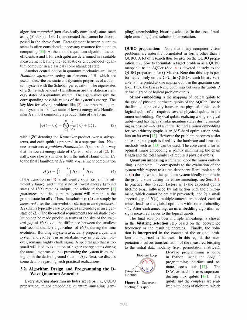
Niobium Loop

Josephson

junction

Figure 2. Supercon-ducting flux qubit.

D-Wave programming is donein Python, using the Leap 2programming interface and re-mote access tools [17]. TheD-Wave machine uses supercon-ducting flux qubits [43]. Thequbits and the couplers are real-ized with loops of niobium, which

7589

have to be cooled to temperatures below 17mK. The cur-rent, that flows clockwise or anti-clockwise through the nio-bium loop can be modeled as a qubit, see Fig. 2. Thus, it ispossible to have a superposition between a current flowingclockwise and anticlockwise as long as no measurement isperformed. The specified couplings J and biases b in (2)determine the time evolution of the magnetic fluxes duringquantum annealing.

3.3. α-Expansion

The α-expansion algorithm was introduced in [10] tosolve labeling optimization problems (e.g., for semanticsegmentation or disparity estimation). A notable extensionis [37], where the method is generalized to allow for par-allel computation amongst other things. In each iteration,a vector of binary variables α that correspond to two pro-posed values for the labels is computed so that the decisionbetween the proposals improves the energy. [10] finds theoptimal expansion through a graph cut such that each pixelin an image is assigned to the first proposed label if αi = 1or the second proposed label if α = 0.

Apart from this application, α-expansion works particu-larly well in case the subproblem, i.e., the optimization forα, is submodular. Then the subproblem can be solved effi-ciently using graph cut techniques.

3.4. Cyclic Permutations

We define the set of permutation matrices as Pn = {X ∈{0, 1}n×n |

∑iXij = 1,

∑j Xij = 1 ∀i, j}. A permuta-

tion matrix X is called a k-cycle, if there exist k many dis-joint indices i1, . . . , ik such thatXi1ik = 1 andXij+1ij = 1for all j = 1, . . . , k−1, andXll = 1 for all l /∈ {i1, . . . , ik},in which case X = (i1 i2 . . . ik) is a common notation.Two permutations X and X ′ are called disjoint if Xii = 1implies X ′

ii = 1 and X ′ii = 1 implies Xii = 1. It is easy

to show that disjoint permutations commute. Furthermore,it holds that any X can be written as the product of 2-cyclesci, i.e., X =

∏Ni=0 ci. Finally, we use the notation X1 = X

and X0 = I where I is the identity for any matrix X .

4. MethodThe main difficulty of previous quantum computing

methods such as [62] for solving (1) is handling the linearequality constraints arising from the optimization over per-mutation matrices. Instead of enforcing them via a penalty,the core idea of Q-Match is to minimize (1) iteratively: Wepropose to use a variant of the α-expansion algorithm thatchooses k-many disjoint candidate cycles ci and uses quan-tum computing to solve the (still NP-hard but smaller andunconstrained) subproblem of deciding whether to apply cior not (identified with αi = 1 and αi = 0, respectively). Inthe following, we detail the idea of the cyclic α-expansionas well as our proposed Q-Match algorithm.

4.1. Cyclic α-Expansion

Let C = {c1, ..., cm} be a set of m disjoint cycles. Weconsider the following optimization problem for an initialpermutation P0:

argmin{P∈Pn|∃α∈{0,1}m: P=(

∏i c

αii )P0}

E(P ), (5)

where E is defined in (1) and α is a binary vectorparametrizing P . As noted in Sec. 3.4, the order in theproduct of all cαi

i does not matter as disjoint permutationscommute. (5) would be equivalent to (1) if C was not fixedwith disjoint cycles but could also be optimized.

Problem complexity: The optimization problem in (5)makes a binary decision for each cycle whether it should beapplied. In this section, we show that (5) is an optimizationproblem with complexity dependent on the number of cy-cles and not n. We can convert the multiplication of cyclesfrom (5) into the following linear combination

P (α) = P0 +

m∑i=1

αi(ci − I)P0, (6)

where I is the identity. See the supplement for a proof.Next, we use this representation to show that (5) is a prob-lem in the form of (2) with size m. Let P,Q be two permu-tations and E(Q,R) = vec(Q)TWvec(R) which is linearin each component. We write Ci = (ci − I)P0 to simplifythe notation. Thus, to solve (5), we need to minimize

E(P0 +∑i

αiCi, P0 +∑j

αjCj)

= E(P0, P0 +∑j

αjCj) +∑i

αiE(Ci, P0 +∑j

αjCj)

= E(P0, P0) +∑j

αjE(P0, Cj) +∑i

αiE(Ci, P0)

+∑i

∑j

αjαiE(Ci, Cj) = E(P0, P0) + αT Wα,

with

Wij =

{E(Ci, Cj) if i = j,

E(Ci, Ci) + E(Ci, P0) + E(P0, Cj) otherwise.(7)

As E(P0, P0) is constant w.r.t. α, we are left with

minα∈{0,1}m

α⊤Wα, (8)

which can be solved directly by AQCers. The interpretationof the optimal α is a binary indicator for whether to applythe corresponding cycle or not. With the basic methodologyof (8) being established, we proceed iteratively: Given acurrent estimate Pi−1 minimizing (1), we choose a set ofdisjoint cycles C = {c1, c2, . . . , cm}, optimize (8), and setPi =

(∏j c

αj

j

)Pi−1.

7590

Algorithm 1: Q-MatchInput: Shapes M,NOutput: Correspondences P

1 Initialize P (Sec. 4.2.3)2 repeat3 Calculate the k worst vertices IM , IN (10)4 Construct sub-matrix of worst matches Ws (S. 4.2.2)5 repeat6 Choose random set of new 2-cycles7 Calculate W (Sec. 4.2.2 and (7))8 Solve the QUBO (8) with AQCing9 Update permutation according to (6)

10 until Every 2-cycle occurred in one set11 Apply permutation to worst vertices in P

12 until P does not change anymore13 return P

4.2. Q-Match

Cyclic α-expansion can optimize any QAP up to a prob-lem size that fits within the AQC, e.g., by iterating over ran-dom sets of cycles. To solve larger problems of (isometric)shape correspondence between two 3D shapes M and N ,we propose Q-Match. If both shapes are discretized withthe same mesh of n vertices, W has the following form:

Wi·n+k,j·n+l = |dgM (i, j)− dgN (k, l)| (9)

where i, j are vertices on M , k, l are vertices on N , anddg(a, b) is the geodesic distance between two points onthe same shape. Therefore, for two matches (i, k), (j, l)Wi·n+k,j·n+l describes how well the geodesic distance ispreserved between the elements of this pair. The optimalsolution is the correspondence for which the distance be-tween all pairs of points is preserved the best, for isome-tries the optimal energy of (1) is zero. Since the geodesicdistances have geometric meaning, this propagates into theQAP, and Q-Match leverages this to choose better sets ofcycles. In Q-Match, the set of tested cycles is based on thecontribution of each vertex to (1) (Sec. 4.2.1), we can solvesubproblems iteratively (Sec. 4.2.2), and the initial permu-tation is descriptor-based (Sec. 4.2.3). An overview of theentire Q-Match algorithm can be found in Alg. 1.

4.2.1 Choosing Cycles

One option to select C is by randomly drawing disjoint cy-cles, which might, however, take many iterations to reachthe optimum. Instead we make use of the fact that the iso-metric shape matching problem creates QAPs in which theentries are highly correlated.

Worst Vertices: For a point with index v in M and a per-mutation P , we can quantify the influence of v on (1) via

I(v) =∑w∈M

Wv·n+P (v),w·n+P (w), (10)

where P (v) denotes the index v is mapped to. For verticeson N we proceed equivalently. If I(v) is high, this is anindicator for P (v) being inconsistent with the majority ofother matches in P . Therefore, we collect the m verticeswith highest values for I on each shape in the two sets IMand IN . The potential improvement of (1) is maximized bythis choice. See Sec. 5.3 for an analysis of the size of m.

2-Cycles: Subsequently, we choose a set of k random butdisjoint 2-cycles from IM , IN . While the limitation to 2-cycles might sound restrictive, the following lemma (provenin the appendix and in many abstract algebra textbooks[60]) highlights the expressive power of disjoint 2-cycles:

Lemma 4.1. Every permutation P can be written as P =QR, where Q and R are products of disjoint 2-cycles.

4.2.2 Subproblems

3D meshes normally consist of more than thousand vertices,this meansW ∈ Rn2×n2

cannot be precomputed and storedin memory. Therefore, in each iteration all needed entries ofW to compute W for (8) have to be computed from scratch.As can be seen in (7) several evaluations of the cost functionE are needed for W which makes this operation expensive.

To be more efficient, we split the computation into thecalculation of Ws, a k2 × k2 reduction of W based on the kworst vertices in IM , IN . This is the most expensive oper-ation in our algorithm (see Fig. 6). For a set of 2-cycles onIM , IN , computing W is now efficient. To reduce the num-ber of times we have to compute Ws, instead of just choos-ing one set of 2-cycles on each IM , IN , we evaluate severalsets. In practice, we sample sets of 2-cycles on IM , IN un-til every possible 2-cycle has been chosen at least once. Adetailed description how to compute Ws and Ws and a run-time analysis can be found in the supplementary material.

4.2.3 Initialization

The only thing left is choosing P0 for the first iteration. In-stead of a random initialization, we calculate a descriptor-based similarity S ∈ RN×N between all vertices of M andN , equivalent to the strategy of [69]. Smn contains the in-ner product of the normalized HKS [65] and SHOT [66] de-scriptors of vertices m ∈ M,n ∈ N , and we solve a linearassignment problem on S to get the first permutation.

7591

2 4 6 8 100

0.5

1

Problem size NProb

abili

tyof

Opt

imal

ity

TwiceOnce

0

0.2

0.4

0.6

0.8

1

2 4 6 8 101214161820# InstancePe

rcen

tage

ofA

nnea

ls Q-MatchQGM [62]

Figure 3. Experiments on how often Q-Match retrieves the opti-mum for (1). (Left) Fraction of random instances with increasingproblem size for which our iterative method leads to the optimumwith brute-force calculation. (Right) Success rate of Q-Match andQGM [62] on 20 random problems. We count (QGM) or lowerbound (ours) the percentage of anneals that reach the optimum.

5. Experiments

We evaluate accuracy, convergence, and runtime ofour method on random QAP instances (Sec. 5.1), FAUST(Sec. 5.2) and QAPLIB (Sec. 5.5). Since quantum comput-ing time is still extremely expensive, we only evaluate onsubsets of FAUST and QAPLIB, but our results show howpromising this technology can be in the future. All experi-ments were done on Intel i5 8265U CPU with 16GB RAMusing Python 3.8 and D-Wave Advantage system 1.1 ac-cessed by Leap 2. Note that one can use classical QUBOsolvers for the subproblems. In the appendix, we presentexperiments for this with a simulated annealing sampler.

5.1. Comparison to Penalty Based Implementation

We compare Q-Match to the inserted method in [62] forproblems of the form (9) with distances di,j drawn uni-formly at random from [0, 1], and W being constructed us-ing a randomly drawn true permutation P . We comparethe success probability of both methods on 20 random in-stances, see Fig. 3-(right). Q-Match finds the optimum inall but 4 cases. For a fair comparison, we restrict the num-ber of anneals per iteration in our method to 10 and use500 anneals for the inserted method. Additionally, the suc-cess probability of the iterative method is bounded by thesuccess probabilities of the individual steps multiplied witheach other. In the case that multiple distinct outputs have thelowest energy, both results will be counted as success. Forn ∈ {2, 4, 6, 8, 10}, we count how often the optimal per-mutation is reached, if each subproblem is solved to globaloptimality. For this we generated 20 random instances forn = 10 and 100 random instances for the other dimen-sions. The errors are calculated as a binomial proportionconfidence interval that should contain the true probabilityin 95% of the cases. This experiment was performed first sothat all 2-cycles occur only once and a second time wherethe whole process is carried out twice, see Fig. 3-(left).

0 5 · 10−2 0.1 0.15 0.20

20

40

60

80

100

Geodesic error

%C

orre

spon

denc

es

FMs [52]SA [28]ZO [44]Q-Match

5 10 150

1

2

3·104

# Iteration

Ene

rgy

(1)

Worst 26Worst 40Worst 50

Figure 4. Evaluation of cumulative error [32] (left) and conver-gence (right) on FAUST. (Left) We compare against Simulated An-nealing [28] without post-processing and Functional Maps [52].Dashed lines indicate non-quantum approaches. The results havesymmetry-flipped solutions removed, these have a comparable fi-nal energy for all methods but are not recognized as correct in theevaluation. (Right) We show convergence of the energy over 30 it-erations. The larger the set of worst vertices, the faster our methodconverges. The dashed grey line shows the optimal energy.

(i) (ii)

Figure 5. Example correspondences from the FAUST registra-tions. (i) Our results are overall correct with some outliers. (ii) Afailure case. The solution partially swapped front and back. Thesekinds of solutions are near-isometries, have energies close to theoptimum, and often occur in all methods that purely solve (1).

Moreover, we study if the solution with the lowest valuereturned by the quantum annealer is globally optimal. For500 runs and coupling matrices up to a size of 13 this wasalways the case. Therefore, the number of optima found byQ-Match is identical to the probabilities in Fig. 3-(left).

5.2. FAUST

We perform experiments on the registrations of theFAUST dataset [7]. We evaluate on 5 different pairs fromone class within FAUST that were downsampled to 502 ver-tices. It is in theory possible to use our method on the orig-inal resolution and more pairs, but QPUs are not as freelyavailable as traditional hardware, and we focus our availablecomputing time on a deeper analysis of our method. We ap-ply Q-Match as described in Alg. 1 with 500 anneals, andcompare to two non-quantum methods, Simulated Anneal-ing [28] and Functional Maps [52]. [28] is applied withoutZoomOut [44] such that it is close to a version of our al-gorithm where only one 2-cycle is chosen in each iteration.The functional maps implementation includes a Laplaciancommutativity regularizer and retrieves the final point-to-

7592

10 15 20 250

20

40

60

# worst vertices

Run

time

(in

ms)

QPU accessCouplings

10 15 20 250

5

10

15

# worst vertices

Run

time

(in

s) Calc. W

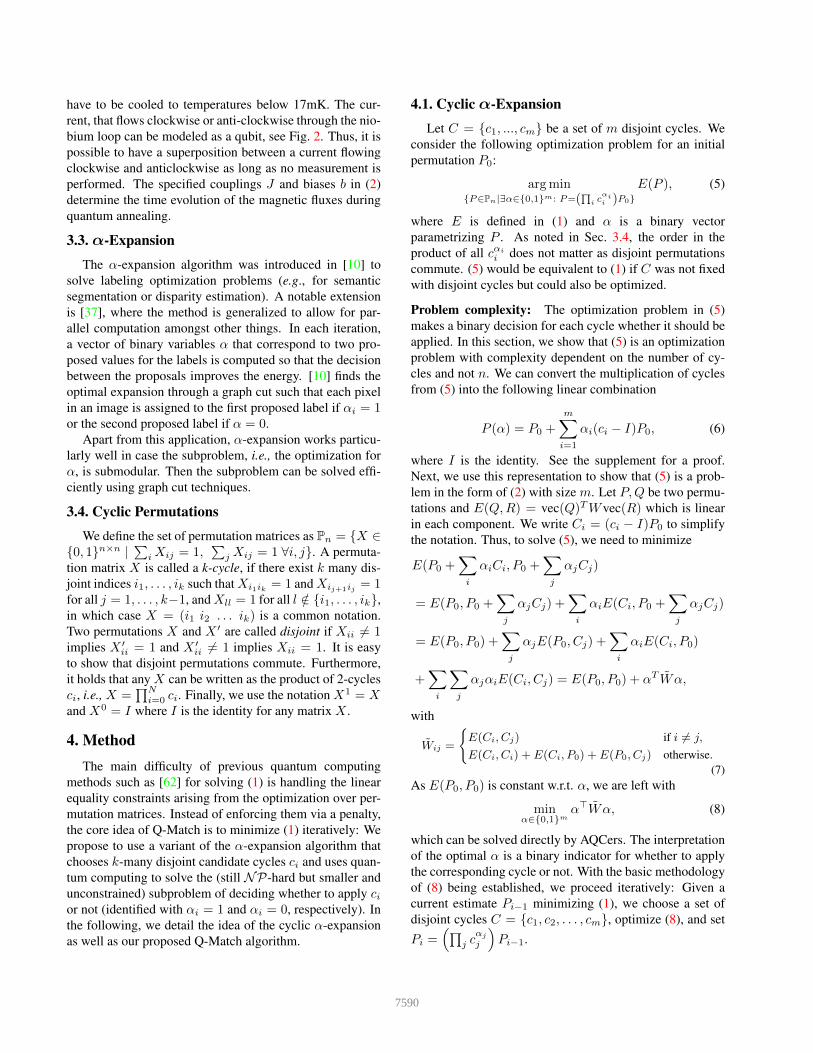
Figure 6. Influence of the problem size on the runtime. We in-crease the size of the set of worst vertices (see Sec. 4.2) and mea-sure the runtime development of different parts of our pipeline.While the QPU access time is mostly independent of the problemsize, calculating W on the CPU grows drastically.

point correspondence through an LAP [52]. While [62] isthe conceptionally closest method to ours, it only producesmatches for up to preselected 4 vertices. The quantitativeevaluation can be seen in Fig. 4, and some qualitative ex-amples of our method in Fig. 5. While we do not reach thesame accuracy as the recent [28], we do outperform the clas-sical but still popular functional maps. Since AQCers arestill newly developed and have limited complexity in com-parison to traditional computers, we see this as a successfulapplication of quantum annealing for real-world problems.

5.3. Convergence

We evaluate how many iterations Q-Match needs to con-verge on FAUST. Fig. 4 shows the convergence when choos-ing 26, 40, 50 worst vertices in each iteration. Since themargin between 40 and 50 is small, we chose to run all fur-ther experiments with the 40 worst matches. In each itera-tion every 2-cycle occurs once in a set C. Some exemplarymatches obtained in this way can be seen in Fig. 5.

5.4. Runtime

Fig. 6 shows how the runtime of Q-Match scales withthe problem size given by the number of worst vertices.The calculation of the submatrix Ws is the most expensive.Computing the matrix W given Ws takes only ms, whilethe calculation of Ws is in the order of seconds. We did notoptimize or parallelize this operation though. The QPU ac-cess time is the time the quantum annealer spends to solvethe problem, and is mostly independent of the problem size.

We report results for about 25 minutes of QPU time,which allows us to evaluate 104 QUBOs. One FAUST in-stance using 40 worst vertices and 500 anneals per QUBOrequires about 2min of QPU time. For all experiments weused the default annealing path and the default annealingtime of 20µs. The chain strength was chosen as 1.0001times the largest absolute value of couplings or biases.

0 2 4 6 80.1

0.5

1

Instance in [12]

Rel

ativ

eer

ror

in%

0 5 1015

10

15

Instance in [61, 25, 56]

0 5 10 15

1

5

10

Instance in [51]

Rel

ativ

eer

ror

in%

0 2 4 6 80

0.51

1.52

2.53

Instance in [21]

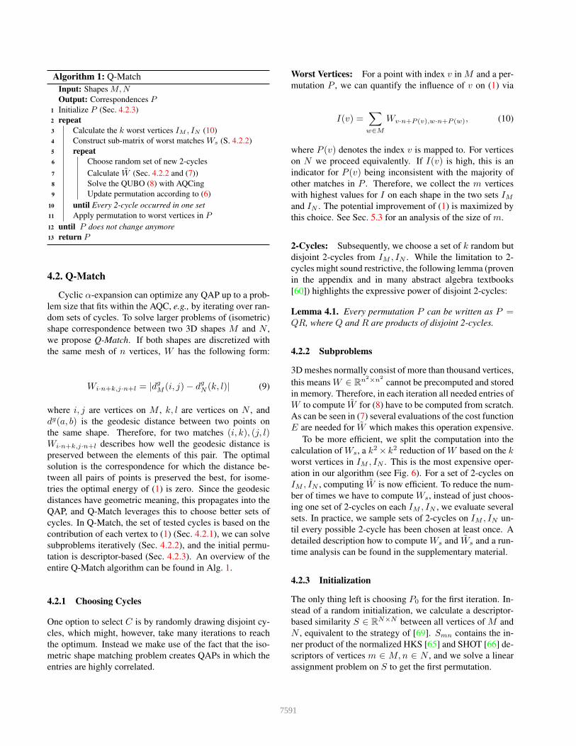
Figure 7. Relative error Eobtained−EoptEopt

of our method in percentagefor the instances of [12], [61] (1-3), [25] (4-8) and [56] (9-11),[51],and [21] in QAPLIB. The problem sizes range between 12 and 30,of which [51] contains the larger ones where we do less well.

5.5. QAPLIB

QAPLIB [11] provides a collection of QAPs togetherwith the best known solution. This is the most commonlyused benchmark for QAPs, with sets of problems from a va-riety of settings, e.g. graphs but also unstructured data. Forsome instances it is unclear if the best known solution isactually the optimum due to the complexity of the problem.

We ran cyclic α-expansion on some of the subsets en-suring that every 2-cycle occurs once when optimizing, andrepeat this three times. We always choose the best solu-tions from 5000 anneals if the size is > 25, and 500 annealsotherwise. The relative error we achieved is in Fig. 7. Forinstances from [12, 21, 25], our solution is almost alwayswithin 1% of the best solution. For the n = 16 instances in[21], we achieved the optimal solution in 9 out of 10 cases.Other sets contain instances up to size 30 and pose a biggerchallenge, our worst result was within 15% of the optimum.We report our exact solutions in the supplementary material.

6. ConclusionWe introduce Q-Match and experimentally show that it

can solve correspondence problems of sizes encountered inpractical applications. This conclusion is made for the firsttime in literature for methods utilizing quantum annealing.Refraining from explicit permutation constraints and ad-dressing the problem iteratively allowed us to significantlyoutperform the previous quantum state of the art, both interms of the supported problem sizes and the probability tomeasure a globally optimal solution. We even achieved re-sults comparable to a classical method. We hope that ourwork inspires further research in quantum annealing and re-lated optimization problems in the vision community.Acknowledgements. This work was partially supported by theERC consolidator grant 4DReply (770784).

7593

References[1] Dorit Aharonov, Wim Van Dam, Julia Kempe, Zeph Landau,

Seth Lloyd, and Oded Regev. Adiabatic quantum computa-tion is equivalent to standard quantum computation. SIAMreview, 50(4):755–787, 2008.

[2] Kurt M. Anstreicher and Nathan W. Brixius. Solvingquadratic assignment problems using convex quadratic pro-gramming relaxations. Optimization Methods and Software,16(1-4):49–68, 2001.

[3] Mathieu Aubry, Ulrich Schlickewei, and Daniel Cremers.The wave kernel signature: A quantum mechanical approachto shape analysis. In International Conference on ComputerVision Workshops (ICCV Workshops), 2011.

[4] Florian Bernard, Christian Theobalt, and Michael Moeller.Ds*: Tighter lifting-free convex relaxations for quadraticmatching problems. In Computer Vision and Pattern Recog-nition (CVPR), 2018.

[5] Dimitri P. Bertsekas. Network Optimization: Continuousand Discrete Models. Athena Scientific, 1998.

[6] Tolga Birdal, Vladislav Golyanik, Christian Theobalt, andLeonidas Guibas. Quantum permutation synchronization. InComputer Vision and Pattern Recognition (CVPR), 2021.

[7] Federica Bogo, Javier Romero, Matthew Loper, andMichael J. Black. Faust: Dataset and evaluation for 3d meshregistration. In Computer Vision and Pattern Recognition(CVPR), 2014.

[8] Max Born and Vladimir Fock. Beweis des adiabatensatzes.Zeitschrift fur Physik, 51(3):165–180, 1928.

[9] Edward Boyda, Saikat Basu, Sangram Ganguly, AndrewMichaelis, Supratik Mukhopadhyay, and Ramakrishna R.Nemani. Deploying a quantum annealing processor to de-tect tree cover in aerial imagery of california. PLoS ONE,12, 2017.

[10] Yuri Boykov, Olga Veksler, and Ramin Zabih. Fast approx-imate energy minimization via graph cuts. IEEE Transac-tions on Pattern Analysis and Machine Intelligence (TPAMI),23(11), 2001.

[11] Rainer E. Burkard, Stefan E. Karisch, and Franz Rendl.Qaplib - a quadratic assignment problem library. Journalof Global Optimization, 1997.

[12] Rainer E. Burkard and Josef Offermann. Entwurfvon schreibmaschinentastaturen mittels quadratischer zuord-nungsprobleme. Zeitschrift fur Operations Research, 1977.

[13] Jun Cai, William G. Macready, and Aidan Roy. A practicalheuristic for finding graph minors. arXiv e-prints, 2014.

[14] Simona Caraiman and Vasile I. Manta. Image processingusing quantum computing. In International Conference onSystem Theory, Control and Computing (ICSTCC), 2012.

[15] Gabriele Cavallaro, Dennis Willsch, Madita Willsch, Kris-tel Michielsen, and Morris Riedel. Approaching remotesensing image classification with ensembles of support vec-tor machines on the d-wave quantum annealer. In IEEEInternational Geoscience and Remote Sensing Symposium(IGARSS), 2020.

[16] Andrew M Childs, Edward Farhi, and John Preskill. Robust-ness of adiabatic quantum computation. Physical Review A,65(1):012322, 2001.

[17] D-Wave Systems, Inc. Leap datasheet v10. https://www.dwavesys.com/sites/default/files/Leap_Datasheet_v10_0.pdf, 2021. online; accessedon the 25.02.2021.

[18] Arnab Das and Bikas K Chakrabarti. Quantum annealingand related optimization methods, volume 679. Springer Sci-ence & Business Media, 2005.

[19] Vasil S. Denchev, Sergio Boixo, Sergei V. Isakov, Nan Ding,Ryan Babbush, Vadim Smelyanskiy, John Martinis, andHartmut Neven. What is the computational value of finite-range tunneling? Phys. Rev. X, 6:031015, Aug 2016.

[20] Roberto Dyke, Caleb Stride, Yu-Kun Lai, Paul L. Rosin,Mathieu Aubry, Amit Boyarski, Alex M. Bronstein,Michael M. Bronstein, Daniel Cremers, and Matthew Fisheret al. Shrec’19: Shape correspondence with isometric andnon-isometric deformations. In Workshop on 3D Object Re-trieval (3DOR), 2019.

[21] Bernhard Eschermann and Hans-Joachim Wunderlich. Op-timized synthesis of self-testable finite state machines. In20th International Symposium on Fault-Tolerant Computing(FFTCS 20), 1990.

[22] Edward Farhi, Jeffrey Goldstone, Sam Gutmann, Joshua La-pan, Andrew Lundgren, and Daniel Preda. A quantum adia-batic evolution algorithm applied to random instances of annp-complete problem. Science, 292(5516):472–475, 2001.

[23] Fajwel Fogel, Rodolphe Jenatton, Francis Bach, and Alexan-dre D' Aspremont. Convex relaxations for permutation prob-lems. In Advances in Neural Information Processing Systems(NeurIPS), volume 26, 2013.

[24] Vladislav Golyanik and Christian Theobalt. A quantum com-putational approach to correspondence problems on pointsets. In Computer Vision and Pattern Recognition (CVPR),2020.

[25] Scott W Hadley, Franz Rendl, and Henry Wolkowicz. Anew lower bound via projection for the quadratic assignmentproblem. Mathematics of Operations Research, 1992.

[26] Peter Hahn, Thomas Grant, and Nat Hall. A branch-and-bound algorithm for the quadratic assignment problem basedon the hungarian method. European Journal of OperationalResearch, 108(3):629–640, 1998.

[27] Oshri Halimi, Or Litany, Emanuele R. Rodola, Alex M.Bronstein, and Ron Kimmel. Unsupervised learning of denseshape correspondence. In Computer Vision and PatternRecognition (CVPR), 2019.

[28] Benjamin Holzschuh, Zorah Lahner, and Daniel Cremers.Simulated annealing for 3d shape correspondence. In Con-ference of 3D Vision (3DV), 2020.

[29] Ibm q experience. https://quantum-computing.ibm.com, 2021. Accessed on the 26.02.2021.

[30] Tadashi Kadowaki and Hidetoshi Nishimori. Quantum an-nealing in the transverse ising model. Phys. Rev. E, 58:5355–5363, 1998.

[31] Itay Kezurer, Shahar Z. Kovalsky, Ronen Basri, and YaronLipman. Tight relaxation of quadratic matching. In Euro-graphics Symposium on Geometry Processing, 2015.

[32] Vladimir G. Kim, Yaron Lipman, and Thomas A.Funkhouser. Blended intrinsic maps. ACM Trans. Graph.,30(4), 2011.

7594

[33] Andrew D King, Jack Raymond, Trevor Lanting, Sergei VIsakov, Masoud Mohseni, Gabriel Poulin-Lamarre, SaraEjtemaee, William Bernoudy, Isil Ozfidan, Anatoly YuSmirnov, et al. Scaling advantage over path-integral montecarlo in quantum simulation of geometrically frustrated mag-nets. Nature Communications, 12(1):1–6, 2021.

[34] Tjalling C. Koopmans and Martin Beckmann. AssignmentProblems and the Location of Economic Activities. Econo-metrica, 25(1):53, Jan. 1957.

[35] Eugene L. Lawler. The quadratic assignment problem. Man-agement science, 9(4):586–599, 1963.

[36] D. Khue Le-Huu and Nikos Paragios. Alternating directiongraph matching. In Computer Vision and Pattern Recogni-tion (CVPR), 2017.

[37] Victor Lempitsky, Carsten Rother, Stefan Roth, and AndrewBlake. Fusion moves for markov random field optimization.IEEE Transactions on Pattern Analysis and Machine Intelli-gence (TPAMI), 32(8):1392–1405, 2010.

[38] Marius Leordeanu and Martial Hebert. A spectral techniquefor correspondence problems using pairwise constraints. InInternational Conference on Computer Vision (ICCV), 2005.

[39] Junde Li and Swaroop Ghosh. Quantum-soft qubo suppres-sion for accurate object detection. In European Conferenceon Computer Vision (ECCV), 2020.

[40] Or Litany, Tal Remez, Emanuele Rodola, Alex Bronstein,and Michael Bronstein. Deep functional maps: Structuredprediction for dense shape correspondence. In InternationalConference on Computer Vision (ICCV), 2017.

[41] Sven Loncaric. A survey on shape analysis techniques. Pat-tern Recognition, 31(8), 1998.

[42] Jonathan Masci, Davide Boscaini, Michael M. Bronstein,and Pierre Vandergheynst. Geodesic convolutional neuralnetworks on riemannian manifolds. In International Con-ference on Computer Vision Workshop (ICCVW), 2015.

[43] Catherine C. McGeoch. Adiabatic quantum computation andquantum annealing: Theory and practice. Synthesis Lectureson Quantum Computing, 5(2):1–93, 2014.

[44] Simone Melzi, Jing Ren, Emanuele Rodola, AbhishekSharma, Peter Wonka, and Maks Ovsjanikov. Zoomout:Spectral upsampling for efficient shape correspondence.ACM Trans. Graph. (Proc. SIGGRAPH Asia), 2019.

[45] Federico Monti, Davide Boscaini, Jonathan Masci,Emanuele Rodola, Jan Svoboda, and Michael M. Bronstein.Geometric deep learning on graphs and manifolds usingmixture model cnns. In Computer Vision and PatternRecognition (CVPR), 2017.

[46] Hartmut Neven, Vasil S. Denchev, Geordie Rose, andWilliam G. Macready. Qboost: Large scale classifier trainingwith adiabatic quantum optimization. In Asian Conferenceon Machine Learning (ACML), 2012.

[47] Hartmut Neven, Geordie Rose, and William G Macready.Image recognition with an adiabatic quantum computer i.mapping to quadratic unconstrained binary optimization.arXiv preprint arXiv:0804.4457, 2008.

[48] Nga T. T. Nguyen and Garrett Kenyon. Image classificationusing quantum inference on the d-wave 2x. In InternationalConference on Rebooting Computing (ICRC), 2018.

[49] Michael A Nielsen and Isaac Chuang. Quantum computationand quantum information, 2002.

[50] Mohammadreza Noormandipour and Hanchen Wang. A pa-rameterised quantum circuit approach to point set matching.arXiv e-prints, 2021.

[51] Christopher E. Nugent, Thomas E. Vollmann, and JohnRuml. An experimental comparison of techniques for theassignment of facilities to locations. Operations Research,1968.

[52] Maks Ovsjanikov, Mirela Ben-Chen, Justin Solomon, AdrianButscher, and Leonidas Guibas. Functional maps: a flexiblerepresentation of maps between shapes. Trans. Graphics,31(4):30, 2012.

[53] Daniel O’Malley, Velimir V. Vesselinov, Boian S. Alexan-drov, and Ludmil B. Alexandrov. Nonnegative/binary matrixfactorization with a d-wave quantum annealer. PLOS ONE,13(12), 12 2018.

[54] Janez Povh and Franz Rendl. Copositive and semidefiniterelaxations of the quadratic assignment problem. DiscreteOptimization, 6(3):231–241, 2009.

[55] Robert Raussendorf and Hans J. Briegel. A one-way quan-tum computer. Phys. Rev. Lett., 86:5188–5191, May 2001.

[56] Catherine Roucairol. Du sequentiel au parallele: larecherche arborescente et son application a la programma-tion quadratique en variables 0 et 1. PhD thesis, UniversitePierre et Marie Curie, 1987.

[57] Catherine Roucairol. A parallel branch and bound algo-rithm for the quadratic assignment problem. Discrete Ap-plied Mathematics, 18(2):211–225, 1987.

[58] Sitapa Rujikietgumjorn and Robert T. Collins. Optimizedpedestrian detection for multiple and occluded people. InComputer Vision and Pattern Recognition (CVPR), 2013.

[59] Samuele Salti, Federico Tombari, and Luigi Di Stefano.Shot: Unique signatures of histograms for surface and tex-ture description. Comput. Vis. Image Underst. (CVIU),125:251–264, 2014.

[60] William Raymond Scott. Group theory. Courier Corpora-tion, 2012.

[61] Michael Scriabin and Roger C. Vergin. Comparison of com-puter algorithms and visual based methods for plant layout.Management Science, 1975.

[62] Marcel Seelbach Benkner, Vladislav Golyanik, ChristianTheobalt, and Michael Moeller. Adiabatic quantum graphmatching with permutation matrix constraints. In Confer-ence of 3D Vision (3DV), 2020.

[63] Justin Solomon, Gabriel Peyre, Vladimir G. Kim, and Su-vrit Sra. Entropic metric alignment for correspondence prob-lems. ACM Trans. Graph., 35(4), 2016.

[64] Bo Sun, Abdullah Iliyasu, Fei Yan, Fangyan Dong, andKaoru Hirota. An rgb multi-channel representation for im-ages on quantum computers. Journal of Advanced Computa-tional Intelligence and Intelligent Informatics, 17:404–417,2013.

[65] Jian Sun, Maks Ovsjanikov, and Leonidas Guibas. A conciseand provably informative multi-scale signature-based on heatdiffusion. Computer Graphics Forum, 2009.

7595

[66] Federico Tombari, Samuele Salti, and Luigi Di Stefano.Unique signatures of histograms for local surface descrip-tion. In European Conference on Computer Vision (ECCV),2010.

[67] Yanghai Tsin and Takeo Kanade. A correlation-based ap-proach to robust point set registration. In European Confer-ence on Computer Vision (ECCV), 2004.

[68] Salvador E. Venegas-Andraca and Sougato Bose. Storing,processing, and retrieving an image using quantum mechan-ics. In Quantum Information and Computation. InternationalSociety for Optics and Photonics, 2003.

[69] Matthias Vestner, Zorah Lahner, Amit Boyarski, Or Litany,Ron Slossberg, Tal Remez, Emanuele Rodola, Alex Bron-stein, Michael Bronstein, Ron Kimmel, and Daniel Cre-mers. Efficient deformable shape correspondence via kernelmatching. In Conference on 3D Vision (3DV), 2017.

[70] Dennis Willsch, Madita Willsch, Hans De Raedt, and KristelMichielsen. Support vector machines on the d-wave quantumannealer. Computer Physics Communications, 248:107006,2020.

[71] Fei Yan, Abdullah M. Iliyasu, and Salvador E. Venegas-Andraca. A survey of quantum image representations. Quan-tum Information Processing, 15(1), 2016.

[72] Qing Zhao, Stefan Karisch, Franz Rendl, and HenryWolkowicz. Semidefinite programming relaxations for thequadratic assignment problem. Journal of CombinatorialOptimization, 2, 10 1997.

7596