Progress in Electromagnetics Research, PIER 26, 89–110, 2000

PULSE PROPAGATION IN SEA WATER:

THE MODULATED PULSE

D. Margetis

Gordon McKay LaboratoryHarvard UniversityCambridge, MA 02138, USA

1. Introduction

2. Formulation

2.1 Preliminaries

2.2 The Low-Frequency Approximation

3. The Modulated Source Pulse: Exact Evaluation of Elfz (ρ, t)

4. Simplified Formulas for Elfz (ρ, t)

5. Discussion and Conclusion

References

1. INTRODUCTION

Electromagnetic fields have long been recognized as a useful tool forgeophysical exploration and remote sensing [1, 2]. Over sixty yearsago, geophysical techniques, particularly the Eltran methods, involvedthe excitation of antennas by current pulses and the subsequent mea-surement of the transient scattered fields in order to extract qualitativeinformation about the dielectric properties of different layers inside theearth [3–5]. In more recent years, electromagnetic pulses are studied inconnection with the optimization of the detection and discriminationof scatterers submerged in dissipative media—specifically, conductingearth and sea water [6, 7]—and even the diagnosis and treatment ofpathologies in biological tissues [8].

When a pulse travels in a dissipative medium, its shape alongwith its characteristics (amplitude, duration, rise and decay time) are

90 Margetis

modified because the complex wave number is no longer linear in fre-quency. Specifically, the large value of conductivity σ in sea waterrenders desirable for remote sensing, as well as for communication withsubmarines, the application of signals whose spectrum has significantcomponents only at very low frequencies. Within this frequency range,a transmitting antenna positioned vertically to and over the boundarybetween air and sea becomes physically impractical because it may notbe made as long as needed to maintain useful properties in the fre-quency domain, an example of such properties being the sufficientlyhigh value of the radiation resistance [9].

A configuration that is often proposed consists of a transmittinghorizontal antenna just below the sea surface [9], where the receiveris chosen to be not too close to the transmitter. Accordingly, the in-coming signal results from the interference of a pulse that reaches thereceiver after propagating downward into the sea, being reflected, andthen propagating upward, with a pulse that travels along the interfacein a surface wave. Of course, the useful signal should be optimally de-tected via continuous cancellation of the second pulse. This task shouldrequire some rather specialized signal-processing techniques and lies be-yond the scope of the present paper.

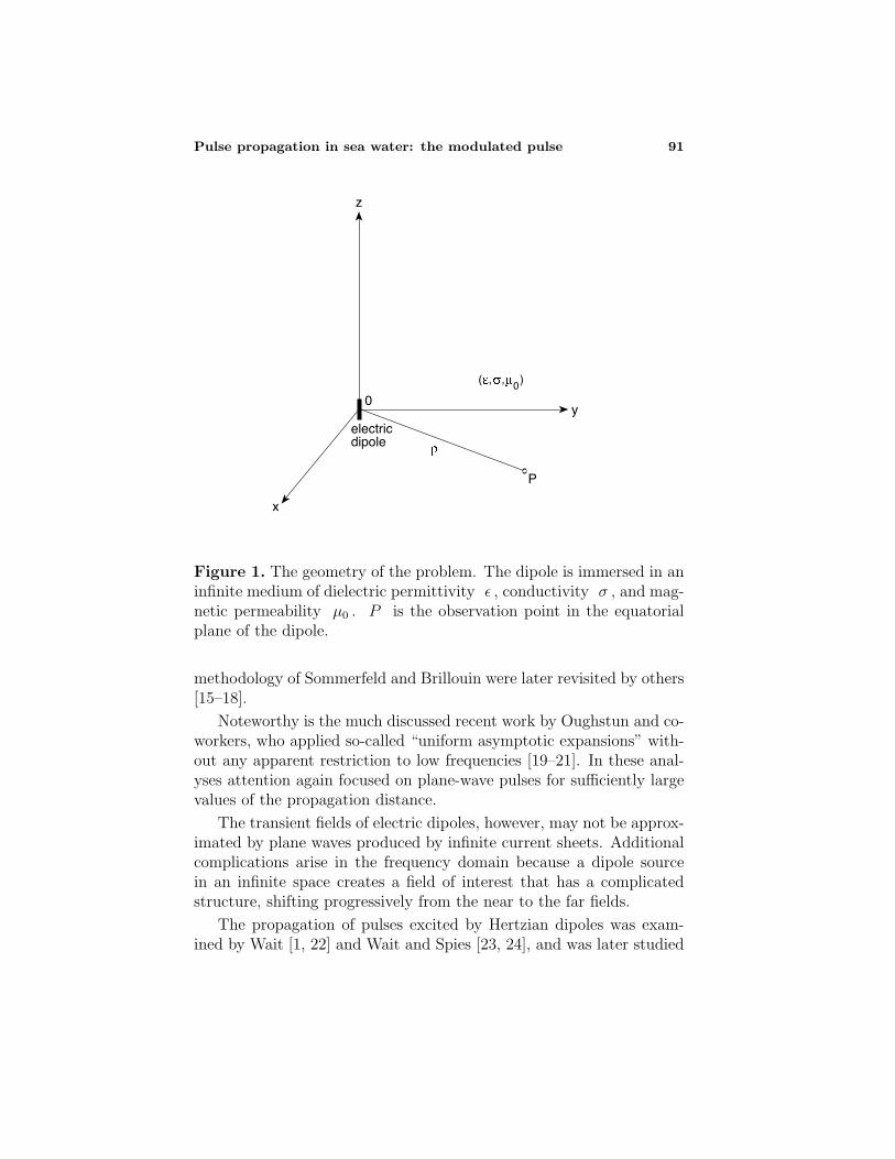
A question that needs to be addressed first is: What is the formof the electromagnetic pulse that travels downward into the sea at anypractical distance from the source, when the current excitation is arealistic function of time? A quantitative answer to this question is astep toward an understanding of how realizable pulses propagate andscatter in highly conducting media and may offer some insight intocertain physical limitations associated with remote sensing. In order tosimplify the analysis in this paper, the horizontal antenna is replaced byan infinitesimal electric dipole oriented along the z-axis and immersedin an infinite medium in the absence of the receiver. The geometry isshown in Fig. 1.

Early advanced analyses of pulse propagation in dispersive mediaby Sommerfeld [10] and Brillouin [11] were motivated by the ques-tion of defining and calculating a signal velocity. These authors stud-ied, asymptotically in distance, the propagation of one-dimensionalplane-wave pulses caused by the sinusoidal modulation of time step-discontinuous boundary conditions in a medium characterized by theLorentz dispersion formula [12]. (See also [13, 14].) The problem and

Pulse propagation in sea water: the modulated pulse 91

z

y

xP

electricdipole0

0)( , ,

Figure 1. The geometry of the problem. The dipole is immersed in aninfinite medium of dielectric permittivity ε , conductivity σ , and mag-netic permeability µ0 . P is the observation point in the equatorialplane of the dipole.

methodology of Sommerfeld and Brillouin were later revisited by others[15–18].

Noteworthy is the much discussed recent work by Oughstun and co-workers, who applied so-called “uniform asymptotic expansions” with-out any apparent restriction to low frequencies [19–21]. In these anal-yses attention again focused on plane-wave pulses for sufficiently largevalues of the propagation distance.

The transient fields of electric dipoles, however, may not be approx-imated by plane waves produced by infinite current sheets. Additionalcomplications arise in the frequency domain because a dipole sourcein an infinite space creates a field of interest that has a complicatedstructure, shifting progressively from the near to the far fields.

The propagation of pulses excited by Hertzian dipoles was exam-ined by Wait [1, 22] and Wait and Spies [23, 24], and was later studied

92 Margetis

systematically under a low-frequency approximation by King [7, 25]and King and Wu [26] in relation to remote sensing in sea water. Theirapproximations are based on the condition σ À ωε , valid for all fre-quencies of interest in sea water. More precisely, with ε ' 80ε0 , whichis the static value of the dielectric permittivity at 20 C [27], andσ ' 4 S/m, the ensuing condition on the frequency f is

f ¿ σ/(2πε) = 9.0× 108 Hz, (1.1)

which poses no practical restriction. Notably, in these works the cur-rent pulse is either a modulated rectangular pulse with an envelope ofzero rise and decay time [25, 26] or a pulse with a gaussian envelopeextending from −∞ to +∞ [7]. The problem of the effect of a finiterise and decay time was addressed by Margetis soon after for the morerealistic excitation pulse [28]

p(t) =1

Tw

(1− e−ωrst)u(t)− [1− e−ωrs(t−Tw)]u(t− Tw). (1.2)

It is the purpose of this paper to extend the analysis of [28] to thecase of a modulated current pulse of the exponential type. The expo-sition is organized as follows. Section 2 revisits the necessary mathe-matical framework and underlying physical principles, with some em-phasis on various subtleties related to the concept of classical causalityand the validity of the low-frequency (or diffusion) approximation. InSec. 3, the electric field in the equatorial plane of the dipole is cal-culated under the low-frequency approximation; the dipole is excitedby a continuously differentiable source pulse of nonzero rise and decaytimes that is modulated by a carrier frequency ω0 . In Sec. 4, sim-ple asymptotic formulas are derived for observation points sufficientlyclose to the source and times of practical interest.

2. FORMULATION

2.1 Preliminaries

As is depicted in Fig. 1, the z-directed dipole is located at the originin an infinite medium with static conductivity σst = σ , static dielec-tric permittivity εst = ε = εrε0 , and magnetic permeability µ = µ0 .

Pulse propagation in sea water: the modulated pulse 93

Maxwell’s equations read

∇× E(r, t) = −∂B(r, t)

∂t, (2.1)

∇×H(r, t) =∂D(r, t)

∂t+ J(r, t), (2.2)

where

J(r, t) = Js(r, t) + Jc(r, t), (2.3)

Js(r, t) = 2heI0p(t)δ(r)z, p(t < 0) = 0, (2.4)

is the source current density, and Jc(r, t) is the conduction currentdensity. p(t) is taken to be bounded with p(t) ≤ O(e−ςt) for t→∞( ς > 0 ). For the frequency range of interest, the constitutive relationsare assumed to be

Jc(r, t) = σE(r, t), (2.5a)

D(r, t) = εE(r, t), H(r, t) =1

µ0

B(r, t). (2.5b)

By virtue of the equation of continuity, −∇ · J = ∂ρ/∂t , it followsthat

∇2E(r, t)− 1

v2

∂2E(r, t)

∂t2=

1

ε∇ρs(r, t) + µ0

∂J(r, t)

∂t, (2.6)

provided that at some fixed time t = t0 ,

∇ · E(r, t0) = ρ(r, t0)/ε. (2.7)

In the above, v = (µ0ε)−1/2 is the velocity of light in the medium

under consideration and ρs(r, t) is the source charge density.It is mathematically convenient to assume the Fourier representa-

tion

E(r, t) =1

2π

∫

Cdω e−iωt E(r, ω), E(r, ω: real) = E∗(r,−ω). (2.8)

What can be said a priori about the contour C is that it shouldbe asymptotically parallel to the real axis and above all singularitiesof E(r, ω) in accord with the fundamental ideas of classical causality.

94 Margetis

This means that at any time t the field quantities for r > 0 aredetermined only by values of Js(r, t) prior to t [12]. In particular,

if p(t) = δ(t), then E(r, t) = 0 for t < 0, (2.9)

E(r, t) corresponding to the known retarded Green’s function for alossless medium when σ = 0 . Attention now focuses on the E(r, t)for which E(r, ω) is holomorphic and bounded in the upper half of theω-plane. Contour C may be taken to coincide with the real axis exceptpossibly in the neighborhood of singular points, such as real poles,where C has to be indented in the upper ω-plane. If the componentEi(r, ω) equals 1, Ei(r, t) becomes the δ-function δ(t) (i = x, y, z).Figure 2 shows the integration path for p(t) = δ(t) .

Clearly, E(r, t) satisfies Eq. (2.6) for |r| > 0 if E(r, ω) obeysthe homogeneous Helmholtz equation

∇2E(r, ω) + k(ω)2E(r, ω) = 0, r > 0, (2.10)

where the complex wave number k(ω) is

k(ω) =√ω2µ0ε+ iωµ0σ = eiπ/4

√ωµ0σ

√1− iωε/σ (2.11)

and a Riemann sheet for the square root is chosen so that

lim|ω|→∞

[k(ω)− ω

v

]=i

2σ

õ0

ε, (2.12)

with the branch-cut configuration of Fig. 2. Of course, contour Cshould lie entirely in this first Riemann sheet.

The calculation of fields is facilitated via the introduction in thetime domain of the conventional vector potential A(r, t) . With thecondition

∇ ·A(r, t) +1

v2

∂Φ(r, t)

∂t+ µ0σΦ(r, t) = 0 (2.13)

and

E(r, t) = −∂A(r, t)

∂t−∇Φ(r, t), (2.14)

the Fourier transform A(r, ω) of A(r, t) is immediately recognized asthe Green’s function for the Helmholtz equation, with the well-knownadmissible solution [29]

A(r, ω) = z 2heI0µ0

4π℘(ω)

eik(ω)r

r. (2.15)

Pulse propagation in sea water: the modulated pulse 95

C

Im

1

i

-plane

C1

t < 0

t > 0

C

Re

C

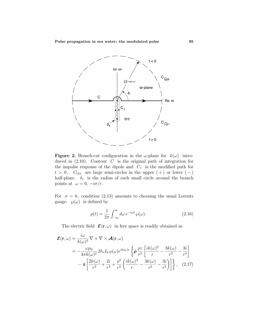
Figure 2. Branch-cut configuration in the ω-plane for k(ω) intro-duced in (2.10). Contour C is the original path of integration forthe impulse response of the dipole and C1 is the modified path fort > 0 . CΩ± are large semi-circles in the upper ( + ) or lower (− )half-plane. δ1 is the radius of each small circle around the branchpoints at ω = 0, −iσ/ε .

For σ = 0 , condition (2.13) amounts to choosing the usual Lorentzgauge. ℘(ω) is defined by

p(t) =1

2π

∫ ∞

−∞dω e−iωt ℘(ω). (2.16)

The electric field E(r, ω) in free space is readily obtained as

E(r, ω) =iω

k(ω)2∇×∇×A(r, ω)

= − ωµ0

4πk(ω)22heI0 ℘(ω)eik(ω)r

ρρz

r2

[ik(ω)2

r− 3k(ω)

r2− 3i

r3

]

− z

[2k(ω)

r2+

2i

r3+ρ2

r2

(ik(ω)2

r− 3k(ω)

r2− 3i

r3

)], (2.17)

96 Margetis

where (ρ, φ, z) are cylindrical coordinates. In the equatorial plane ofthe dipole, z = 0 , the complex electric field is of maximum magnitude:

E(x, y, z = 0, ω)

= zEz(ρ, ω)

= zωµ0

4π(2heI0)℘(ω)eik(ω)ρ

[i

ρ− 1

k(ω)ρ2− i

k(ω)2ρ3

]. (2.18)

2.2 The Low-Frequency Approximation

Since only low frequencies are of interest in sea water, it is reasonableto invoke condition (1.1) and approximate k(ω) as

k(ω) ∼ (iωµ0σ)1/2 = (1 + i)a√ω, a =

√µ0σ/2, (2.19)

in a Lorentz frame where the source does not move.This approximation amounts to the neglect of the displacement

current −iωεE(r, ω) in comparison with the conduction currentσE(r, ω) . In the time domain, the fields are subject to the correspond-ing condition ∣∣∣∣∣

∂D(r, t)

∂t

∣∣∣∣∣¿ σ|E(r, t)|. (2.20)

The sequence of steps that previously furnished Eq. (2.6) now leads to

∇2Elf(r, t) = µ0σ∂Elf

∂t, E ∼ Elf , r > 0, (2.21)

which reduces to Fick’s second (or diffusion) equation for each Carte-sian component of Elf . Analogies between the propagation of low-frequency pulses in highly conducting media and the conduction ofheat in thermal bodies are easily drawn from this equation.

Equation (2.18) under approximation (2.19) gives

E lfz (ρ, ω) =

µ0

2πheI0 ℘(ω)

[iω

ρ− (1− i)√ω

2aρ2− 1

2a2ρ3

]eiaρ

√ωe−aρ

√ω.

(2.22)

Accordingly, the time-dependent field reads

E lfz (ρ, t) =

1

2π

∫ ∞

−∞dω e−iωt E lf

z (ρ, ω)

=µ0heI0

4π

[I1(ρ, t)

ρ+I2(ρ, t)

aρ2+I3(ρ, t)

a2ρ3

], (2.23)

Pulse propagation in sea water: the modulated pulse 97

where

I1(ρ, t) =1

π

∫ ∞

−∞dω e−iωt iω℘(ω)e−(1−i)aρ√ω, (2.24)

I2(ρ, t) =i− 1

2π

∫ ∞

−∞dω e−iωt

√ω ℘(ω)e−(1−i)aρ√ω, (2.25)

I3(ρ, t) = − 1

2π

∫ ∞

−∞dω e−iωt ℘(ω)e−(1−i)aρ√ω. (2.26)

The integration path here is indented in the upper ω-plane aroundsingularities that lie in the real axis, in accord with classical causality.The first Riemann sheet is chosen so that

√ω > 0 for ω > 0 and

the branch cut is taken to coincide with the negative imaginary axis,for instance, by letting ε→ 0+ in Fig. 2. Note that

I2(ρ, t) = −1

a

∂I3(ρ, t)

∂ρ, (2.27a)

I1(ρ, t) = 2∂I3(ρ, t)

∂t, (2.27b)

by interchanging the order of integration and differentiation on thegrounds of an assumed uniform in t and ρ > 0 convergence of theintegrals for I1(ρ, t) , I2(ρ, t) , and I3(ρ, t) . Hence, it is sufficient toevaluate only I3(ρ, t) .

A word of caution about Eq. (2.21) in comparison to the originalEq. (2.6) is now in order. While the latter allows only for electro-magnetic pulses that propagate with velocity which is not greater thanthe (finite) velocity of light (µ0ε)

−1/2 , the former admits solutionsthat propagate instantaneously everywhere in space. However, the useof this equation should pose no practical limitation for distances andtimes of interest in sea water.

As is discussed in more technical detail in [30], approximation (2.19)in the frequency domain implies minimally the conditions

tÀ ρ/v, tÀ τ0 = ε/σ, tÀ ρ

v(ζρ)1/3 (2.28)

in the time domain. Because

τ0 ' 0.18 ns, ζ ≡ −i lim|ω|→∞

[k(ω)− ω

v

]=

1

2σ

õ0

ε' 84.26 m−1

(2.29)

98 Margetis

in sea water ( σ ' 4 S/m , ε ' 80ε0 ), the aforementioned conditionsare of no practical restriction.

3. THE MODULATED SOURCE PULSE: EXACTEVALUATION OF Elf

z (ρ, t)

Consider the current pulse

p(t) =1

Tw

(1− e−ωrst)u(t)− [1− e−ωrs(t−Tw)]u(t− Tw)

sinω0t, (3.1)

where ω0ε/σ ¿ 1 . To ensure that p(t) is a continuously differentiablefunction of time, the width Tw and the period T0 = 2π/ω0 are chosento satisfy the relation

Tw/T0 = n/2, n = 1, 2, 3, . . . . (3.2)

Both Tw and T0 are assumed to be large compared to the right-handsides of conditions (2.28). The Fourier transform of p(t) is

℘(ω) = − 1

2iTw

[℘0(ω − ω0)− ℘0(ω + ω0)][(−1)neiωTw − 1] (3.3a)

= −ωrsω0

iTw

2ω + iωrs(ω2 − ω2

0)[(ω + iωrs)2 − ω20]

[(−1)neiωTw − 1], (3.3b)

where

℘0(ω) =1

ω

ωrsω + iωrs

=1

i

(1

ω− 1

ω + iωrs

). (3.4)

With Eqs. (2.23–2.26), Ij(ρ, t) , j = 1, 2, 3, read

Ij(ρ, t) = T−1w [(−1)nIj(ρ, t− Tw)− Ij(ρ, t)], (3.5)

I1(ρ, t) = − 1

2π

∫ ∞

−∞dω ω[℘0(ω − ω0)− ℘0(ω + ω0)]

× e−(1−i)aρ√ωe−iωt, (3.6)

I2(ρ, t) = −1 + i

4π

∫ ∞

−∞dω√ω [℘0(ω − ω0)− ℘0(ω + ω0)]

× e−(1−i)aρ√ωe−iωt, (3.7)

I3(ρ, t) =1

4πi

∫ ∞

−∞dω [℘0(ω − ω0)− ℘0(ω + ω0)]

× e−(1−i)aρ√ωe−iωt. (3.8)

Pulse propagation in sea water: the modulated pulse 99

0

-plane

0 – i rs0 – i rs

0 0

Im

Re

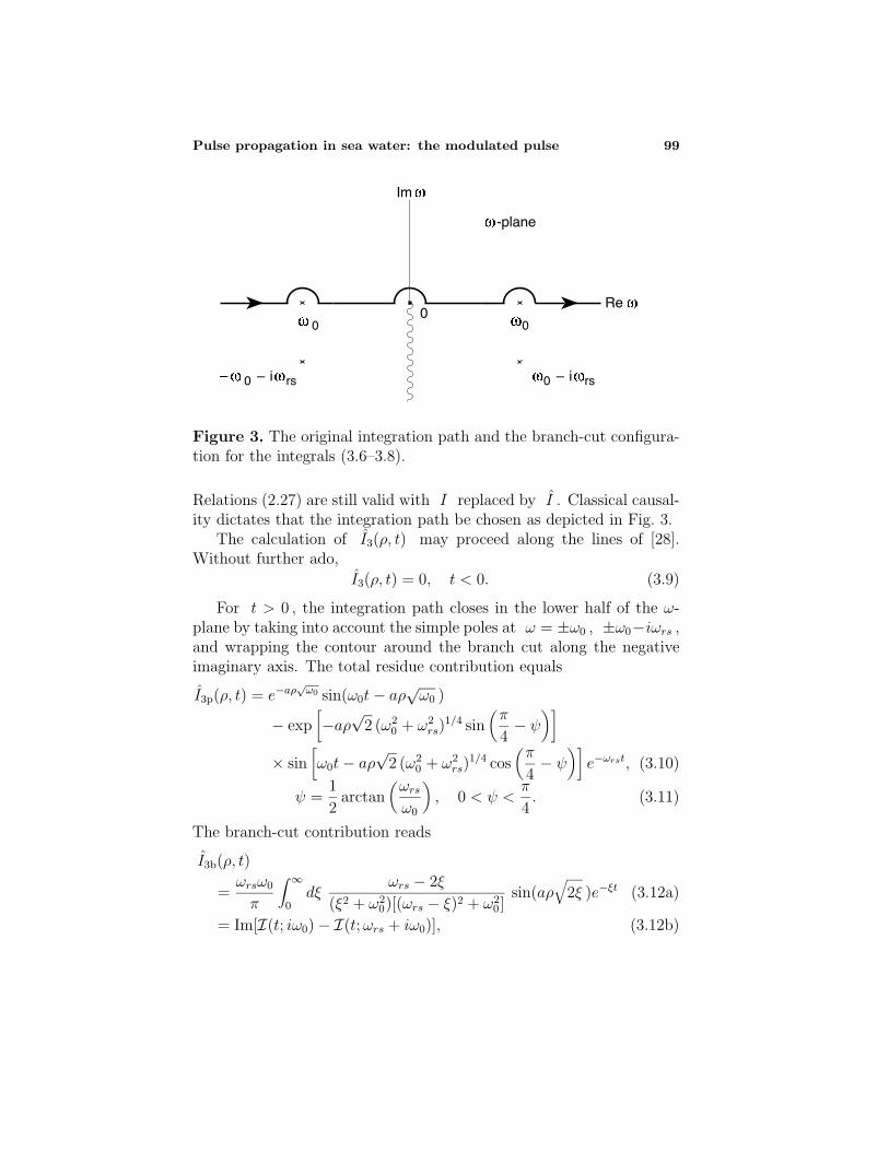
Figure 3. The original integration path and the branch-cut configura-tion for the integrals (3.6–3.8).

Relations (2.27) are still valid with I replaced by I . Classical causal-ity dictates that the integration path be chosen as depicted in Fig. 3.

The calculation of I3(ρ, t) may proceed along the lines of [28].Without further ado,

I3(ρ, t) = 0, t < 0. (3.9)

For t > 0 , the integration path closes in the lower half of the ω-plane by taking into account the simple poles at ω = ±ω0 , ±ω0−iωrs ,and wrapping the contour around the branch cut along the negativeimaginary axis. The total residue contribution equals

I3p(ρ, t) = e−aρ√ω0 sin(ω0t− aρ

√ω0 )

− exp[−aρ√

2 (ω20 + ω2

rs)1/4 sin

(π

4− ψ

)]

× sin[ω0t− aρ

√2 (ω2

0 + ω2rs)

1/4 cos(π

4− ψ

)]e−ωrst, (3.10)

ψ =1

2arctan

(ωrsω0

), 0 < ψ <

π

4. (3.11)

The branch-cut contribution reads

I3b(ρ, t)

=ωrsω0

π

∫ ∞

0dξ

ωrs − 2ξ

(ξ2 + ω20)[(ωrs − ξ)2 + ω2

0]sin(aρ

√2ξ )e−ξt (3.12a)

= Im[I(t; iω0)− I(t;ωrs + iω0)], (3.12b)

100 Margetis

where

I(t;λ) =1

π

∫ ∞

0

dξ

ξ − λ e−ξt sin(aρ√

2ξ ), Im λ > 0. (3.13)

By virtue of

∫ ∞

0dξ e−ξt sin(aρ

√2ξ )

= −√

2

tRe

[∂

∂(aρ)e−a

2ρ2/(2t)∫ ∞

−iaρ/√

2tds e−s

2

]

= aρ

√π

2t3e−a

2ρ2/(2t), (3.14)

I(t;λ) satisfies the differential equation

∂I(t;λ)

∂t+ λI(t;λ) = −aρ(2πt3)−1/2e−a

2ρ2/(2t). (3.15)

This is readily integrated to give

I(t;λ) = I(t = 0+;λ)e−λt

− 2e−λtaρ(2πt)−1/2∫ ∞

1dx exp

(λt

x2− a2ρ2

2tx2

). (3.16)

A straightforward application of Cauchy’s integral formula gives

I(t = 0+;λ) =1

2πi

∫ ∞

−∞dy

y

y2 − λ eiaρ√

2 y −∫ ∞

−∞dy

y

y2 − λ e−iaρ

√2 y

= eiaρ√

2λ. (3.17)

In consideration of the identity

exp

(λt

x2−R2x2

)=

1

2R

d

dx

(e−2i

√λtR

∫ Rx−i√λt/x

0ds e−s

2

+ e2i√λtR

∫ Rx+i√λt/x

0ds e−s

2

), (3.18)

Pulse propagation in sea water: the modulated pulse 101

it is found that

I(t;λ) = eiaρ√

2λe−λt − 1

2e−R

2[e(R+i

√λt )2

erfc(R + i√λt )

+ e(R−i√λt )2

erfc(R− i√λt )

]. (3.19)

The square root is positive for λ > 0 and the branch cut lies in thelower λ-plane, while

R ≡ R(ρ, t) =aρ√2t, (3.20)

as is expected by the similarity solutions of Eq. (2.21), and erfc is thecomplementary error function [31]

erfc(z) =2√π

∫ ∞

zds e−s

2

. (3.21)

It follows from Eq. (3.12b) that

I3b(ρ, t) = −I3p(ρ, t) +1

2e−R

2

[G(Z+) +G(Z−)−G(Z0+)−G(Z0−)],

(3.22)

where

G(Z) = Im[eZ2

erfc(Z)], (3.23)

and

Z± ≡ Z±(ρ, t) = R± i√ωrst+ iω0t

= R∓ [(ω0t)2 + (ωrst)

2]1/4e−i(π/4+ψ), (3.24a)

Z0± ≡ Z0±(ρ, t) = R± i√iω0t = R∓

√ω0t e

−iπ/4. (3.24b)

Hence,

I3(ρ, t) =1

2e−R

2

[G(Z+) +G(Z−)−G(Z0+)−G(Z0−)], t > 0.

(3.25)

I2(ρ, t) and I1(ρ, t) are obtained from Eqs. (2.27):

I2(ρ, t) =1

2e−R

2(√

ω0 [F (Z0+)− F (Z0−)−G(Z0+) +G(Z0−)]

−√

2 (ω20 + ω2

rs)1/4cos(π/4− ψ)[F (Z+)− F (Z−)]

− sin(π/4− ψ)[G(Z+)−G(Z−)]), (3.26)

I1(ρ, t) = e−R2 ω0[F (Z0+) + F (Z0−)− F (Z+)− F (Z−)]

− ωrs[G(Z+) +G(Z−)] , t > 0, (3.27)

102 Margetis

where

F (Z) = Re[eZ2

erfc(Z)]. (3.28)

Note that in the limit ω0 → 0+ all Ij(ρ, t) tend to vanish, as theyshould.

A final exact expression for E lfz (ρ, t) easily follows from Eqs. (2.23)

and (3.5):

E lfz (ρ, t) = −µ0aheI0

8πTw

0, t ≤ 0,e(ρ, t), 0 < t ≤ Tw,e(ρ, t)− (−1)n e(ρ, t− Tw), t > Tw,

(3.29)

where

e(ρ, t) =e−R

2

(2t)3/2

4Ω2

0[F (Z0+) + F (Z0−)− F (Z+)− F (Z−)]

− 4Ω2rs[G(Z+) +G(Z−)]

+ Ω0

√2[F (Z0+)− F (Z0−)−G(Z0+) +G(Z0−)]

− 2(Ω40 + Ω4

rs)1/4(cos(π/4− ψ)[F (Z+)− F (Z−)]

− sin(π/4− ψ)[G(Z+)−G(Z−)])

+G(Z+) +G(Z−)−G(Z0+)−G(Z0−), (3.30)

and R , Z± and Z0± are defined by Eqs. (3.20) and (3.24).

4. SIMPLIFIED FORMULAS FOR Elfz (ρ, t)

A practically appealing case arises when ω0t À 1 for 0 < t < Tw

(ω0Tw À 1 ) or ω0(t−Tw)À 1 for t > Tw . Instead of employing thelarge-argument approximation for the complementary error function inEqs. (3.29–3.30), it is more advantageous to have recourse to the inte-gral of Eq. (3.12a). The change of variable ξ = R2ξ2/t recasts thisintegral in the form

I3b(ρ, t)

=Ω2

0Ω2rs

π

∫ ∞

−∞dξ ξ

Ω2rs − 2ξ2

(ξ4 + Ω40)[(Ω2

rs − ξ2)2 + Ω40]

sin(2R2ξ)e−R2ξ2

=Ω2

0Ω2rs

πe−R

2

Im∫ ∞

−∞dξ ξ

Ω2rs − 2ξ2

(ξ4 + Ω40)[(Ω2

rs − ξ2)2 + Ω40]e−R

2(ξ−i)2

.

(4.1)

Pulse propagation in sea water: the modulated pulse 103

In the above,

Ω0 =

√ω0t

R, Ωrs =

√ωrst

R. (4.2)

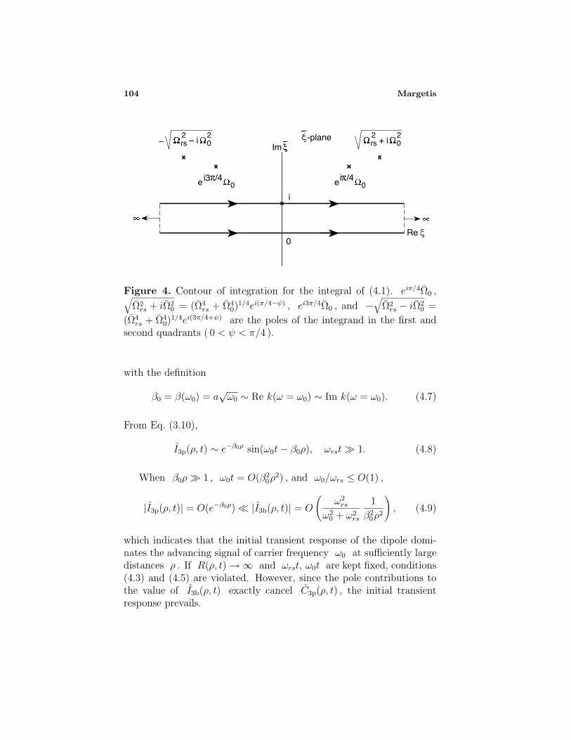
The integration path is shifted parallel to the real axis so that itfinally passes through ξ = i , as shown in Fig. 4. The condition

R =aρ√2t< [(ω0t)

2 + (ωrst)2]1/4 sin(π/4− ψ), (4.3)

along with R <√ω0t/2 , where ψ is defined by Eq. (3.11), ensure

that the contour does not enclose any poles of the integrand. Note thatthe total contribution from these poles would exactly cancel I3p(ρ, t)of Eq. (3.10). With the change of variable R(ξ − i) = x ( x : real )along the new path, I3b(ρ, t) reads

I3b(ρ, t) =Ω2

0Ω2rs

πRe−R

2

Im∫ ∞

−∞dx (i+ x/R)

× Ω2rs − 2(i+ x/R)2

[(i+ x/R)4 + Ω40][Ω2

rs − (i+ x/R)2]2 + Ω40e−x

2

. (4.4)

The contribution to integration from the region x: |x| À 1 is rec-ognized as negligibly small. It follows that if

R2 < O(ω0t), R2 < O(ωrst), ω0t, ωrstÀ 1, (4.5)

the rational function in the integrand can be approximated as

Ω2rs − 2(i+ x/R)2

[(i+ x/R)4 + Ω40][Ω2

rs − (i+ x/R)2]2 + Ω40∼ Ω2

rs

Ω40(Ω4

rs + Ω40)

=ωrs

ω20(ω2

0 + ω2rs)

and pulled out of the integral. Therefore, under conditions (4.5) and(4.3), I3b(ρ, t) becomes

I3b(ρ, t) ∼ ω2rs

πω0(ω2rs + ω2

0)

∫ ∞

0dξ sin(aρ

√2ξ )e−ξt

=ω2rs

ω20 + ω2

rs

β0ρ√2π (ω0t)3/2

e−(β0ρ)2/(2ω0t), (4.6)

104 Margetis

0

ei /4 0ei3 /4

0 i

0+ i

rs 22 0– i rs 22–

Im

Re

-plane

Figure 4. Contour of integration for the integral of (4.1). eiπ/4Ω0 ,√Ω2rs + iΩ2

0 = (Ω4rs + Ω4

0)1/4ei(π/4−ψ) , ei3π/4Ω0 , and −√

Ω2rs − iΩ2

0 =

(Ω4rs + Ω4

0)1/4ei(3π/4+ψ) are the poles of the integrand in the first andsecond quadrants ( 0 < ψ < π/4 ).

with the definition

β0 = β(ω0) = a√ω0 ∼ Re k(ω = ω0) ∼ Im k(ω = ω0). (4.7)

From Eq. (3.10),

I3p(ρ, t) ∼ e−β0ρ sin(ω0t− β0ρ), ωrstÀ 1. (4.8)

When β0ρÀ 1 , ω0t = O(β20ρ

2) , and ω0/ωrs ≤ O(1) ,

|I3p(ρ, t)| = O(e−β0ρ)¿ |I3b(ρ, t)| = O

(ω2rs

ω20 + ω2

rs

1

β20ρ

2

), (4.9)

which indicates that the initial transient response of the dipole domi-nates the advancing signal of carrier frequency ω0 at sufficiently largedistances ρ . If R(ρ, t)→∞ and ωrst, ω0t are kept fixed, conditions(4.3) and (4.5) are violated. However, since the pole contributions tothe value of I3b(ρ, t) exactly cancel C3p(ρ, t) , the initial transientresponse prevails.

Pulse propagation in sea water: the modulated pulse 105

I3(ρ, t) is expressed as

I3(ρ, t) = I3p(ρ, t) + I3b(ρ, t)

∼ e−β0ρ sin(ω0t− β0ρ) + e−a2ρ2/(2t) ω2

rsaρ

ω0(ω2rs + ω2

0)(2πt3)−1/2.

(4.10)

Note that the effect of the rise time τrs = ω−1rs is the decrease of the

transient amplitude by the factor ω2rs/(ω

2rs+ω

20) . I2(ρ, t) and I1(ρ, t)

are approximated by

I2(ρ, t) ∼ √ω0 e−β0ρ [sin(ω0t− β0ρ ) + cos(ω0t− β0ρ )]

+ e−a2ρ2/(2t) ω2

rs

ω0(ω2rs + ω2

0)(2πt3)−1/2

(a2ρ2

t− 1

), (4.11)

I1(ρ, t) ∼ 2ω0e−β0ρ cos(ω0t− β0ρ)

+ e−a2ρ2/(2t) ω2

rsaρ

ω0(ω2rs + ω2

0)(2πt5)−1/2

(a2ρ2

t− 3

). (4.12)

The corresponding approximate formula for E lfz (ρ, t) is

E lfz (ρ, t) ∼ −µ0heI0β0ω0

4πTw

×

0, t ≤ 0,

e−β0ρ

[1

(β0ρ)3+

1

(β0ρ)2

]sin(ω0t− β0ρ)

+

[1

(β0ρ)2+

2

β0ρ

]cos(ω0t− β0ρ)

+2ω2

rs

ω20 + ω2

rs

1√2π(ω0t)5

[(β0ρ)2

2ω0t− 1

]e−(β0ρ)2/(2ω0t),

0 < t ≤ Tw, ω0,rstÀ 1,

2ω2rs

ω20 + ω2

rs

1√

2π(ω0t)5

[(β0ρ)2

2ω0t− 1

]e−(β0ρ)2/(2ω0t)

+ (−1)n+1 1√2π[ω0(t− Tw)]5

e−(β0ρ)2/[2ω0(t−Tw)]

×[

(β0ρ)2

2ω0(t− Tw)− 1

], ω0,rs(t− Tw)À 1.

(4.13)

Note that the sinusoidal signal is exactly cancelled for t > Tw .

106 Margetis

The formula for E lfz (ρ, t) is simplified considerably when β0ρ¿ 1 :

E lfz (ρ, t) ∼ −µ0heI0β0ω0

4πTw

×

0, t ≤ 0,1

(β0ρ)3sin(ω0t− β0ρ)

− 2ω2rs

ω20 + ω2

rs

1√2π(ω0t)5

, 0 < t ≤ Tw, ω0,rstÀ 1,

− 2ω2rs

ω20 + ω2

rs

1√2π

1√

(ω0t)5

+(−1)n+1

√ω5

0(t− Tw)5

, ω0,rs(t− Tw)À 1.

(4.14)

Note that the field close to the dipole is essentially an out-of-phasereplica of the current source pulse, as expected by inspection of Eq.(2.22).

When R(ρ, t) À 1 and R(ρ, t − Tw) À 1 for t > Tw , E lfz (ρ, t)

becomes

E lfz (ρ, t) ∼ −µ0heI0β0ω0

4πTw

×

0, t ≤ 0,

e−β0ρ2

β0ρcos(ω0t− β0ρ)

+ω2rs

ω20 + ω2

rs

e−a2ρ2/(2t)

√2π(ω0t)5

a2ρ2

t,

R(ρ, t)À 1,0 < t ≤ Tw,

ω2rs

ω20 + ω2

rs

e−a2ρ2/(2t)

√2π(ω0t)5

a2ρ2

t

+ (−1)n+1 e−a2ρ2/[2(t−Tw)]

√2π[ω0(t− Tw)]5

a2ρ2

t− Tw

,

R(ρ, t− Tw)À 1,t > Tw.

(4.15)

According to formulas (4.14) and (4.15), the field for 0 < t < Tw shiftsfrom the form of the original source pulse when β0ρ¿ 1 to the formof its time derivative when R(ρ, t)À 1 .

Evidently, the condition ωrs À ω0 and the subsequent approxima-tion ω2

rs

ω20 + ω2

rs

∼ 1

Pulse propagation in sea water: the modulated pulse 107

reduce formula (4.13) to that for the low-frequency field generated bythe rectangular wave packet [26]

p(t) =1

Tw

[u(t)− u(t− Tw)] sinω0t.

5. DISCUSSION AND CONCLUSION

The present paper concludes previous work by the same author on thepropagation of electromagnetic pulses excited by exponential currentswith finite rise and decay times [28]. The electric field created by aHertzian dipole in sea water is evaluated analytically under the low-frequency approximation, when the source current is a modulated expo-nential pulse. The fact that the requisite integrals can be carried outexactly depends crucially on the Fourier transform ℘(ω) of the excita-tion pulse p(t) being a meromorphic function of ω . The results ob-tained hitherto can be extended by mere inspection to many-parameterexcitations that ensue from acting successively on the pulse of Eq. (1.2)with conventional low-pass filters (for instance, resistor-capacitor cir-cuits) and modulating the output signal. In view of Mittag-Leffler’stheorem [32], any signal that is constructed by prescribing the loca-tion of poles and the singular parts of ℘(ω) at those poles admits alow-frequency response as a suitable combination of real and imaginaryparts of the complementary error function with complex arguments.

The sinusoidal signal is superimposed to the original transient,shifting successively from the form of the excitation current whenR(ρ, t) ¿ 1 to its time derivative when R(ρ, t) À 1 and the tran-sients tend to dominate the advancing wavepacket. The finite rise anddecay time τrs = ω−1

rs modifies the amplitude of the transient by themultiplicative factor ω2

rs(ω20 + ω2

rs)−1 . Because the exposition is based

on the simplifying condition ωε/σ ¿ 1 in the frequency domain, theanalytical results here are by no means restrictive to sea water but canalso be applied to any other highly conducting medium.

ACKNOWLEDGEMENT

The author is grateful to Professor Ronold W. P. King for suggestingthe problem. He also wishes to thank Margaret Owens for her assistancethroughout the preparation of the manuscript.

108 Margetis

REFERENCES

1. Wait, J. R., “Electromagnetic fields of sources in lossy media,”Chap. 24 in Antenna Theory, Part 2, R. E. Collin and F. J. Zucker,Eds., McGraw-Hill, New York, 438–514, 1969.

2. Wait, J. R., Geo-Electromagnetism, Academic Press, New York,1982.

3. Statham, L., “Electric earth transients in geophysical prospect-ing,” Geophysics, Vol. 1, 271–277, 1936.

4. Hawley, P. F., “Transients in electrical prospecting,” Geophysics,Vol. 3, 247–257, 1938.

5. Klipsch, P. W., “Recent developments in Eltran prospecting,”Geophysics, Vol. 4, 283–291, 1939.

6. Song, J., and K.-M. Chen, “Propagation of EM pulses excited byan electric dipole in a conducting medium,” IEEE Trans. Anten-nas Propagat., Vol. AP-41, 1414–1421, 1993.

7. King, R. W. P., “The propagation of a Gaussian pulse in sea waterand its application to remote sensing,” IEEE Trans. Geosci. &Remote Sens., Vol. GE-31, 595–605, 1993.

8. Pilla, A. A., “State of the art in electromagnetic therapeutics,”Electricity and Magnetism in Biology and Medicine, M. Blank,Ed., San Francisco Press, San Francisco, 1993.

9. King, R. W. P., M. Owens, and T. T. Wu, Lateral ElectromagneticWaves: Theory and Applications to Communications, GeophysicalExploration, and Remote Sensing, Chaps. 5, 7, and 14, Springer-Verlag, New York, 1992.

10. Sommerfeld, A.,“Uber die Fortpflanzung des Lichtes in dis-pergierenden Medien,” Ann. Physik. (Leipzig), Vol. 44, 177–202,1914.

11. Brillouin, L., “Uber die Fortpflanzung des Licht in dispergierendenMedien,” Ann. Physik (Leipzig), Vol. 44, 203–240, 1914.

12. Nussenzveig, H. M., Causality and Dispersion Relations, 43–47,Academic Press, San Diego, 1972.

13. Sommerfeld, A., Optics, Chap. III, Academic Press, New York,1954.

14. Brillouin, L., Wave Propagation and Group Velocity, AcademicPress, San Diego, 1960.

15. Baerwald, H., “Uber die Fortpflanzung von Signalen in dis-pergierenden Systemen,” Ann. Physik, Vol. 7, 731–760, 1930.

16. Bloch, S. C., “Eighth velocity of light,” Amer. J. Phys., Vol. 45,538–549, 1977.

Pulse propagation in sea water: the modulated pulse 109

17. Trizna, D. B., and T. A. Weber, “Brillouin revisited: Signal ve-locity definition for pulse propagation in a medium with resonantanomalous dispersion,” Radio Sci., Vol. 17, 1169–1180, 1982.

18. Chu, S., and S. Wong, “Linear pulse propagation in an absorbingmedium,” Phys. Rev. Lett., Vol. 48, 738–741, 1982.

19. Oughstun, K. E., and G. C. Sherman, “Uniform asymptotic de-scription of electromagnetic pulse propagation in a linear disper-sive medium with absorption (the Lorentz medium),” J. Opt. Soc.Am. A, Vol. 6, 1394–1420, 1989.

20. Oughstun, K. E., and G. C. Sherman, “Uniform asymptotic de-scription of ultrashort rectangular optical pulse propagation in alinear, causally dispersive medium,” Phys. Rev. A, Vol. 41, 6090–6113, 1990.

21. Oughstun, K. E., “Pulse propagation in a linear, causally disper-sive medium,” Proc. IEEE, Vol. 79, 1379–1389, 1991.

22. Wait, J. R., “Transient electromagnetic propagation in a conduct-ing medium,” Geophysics, Vol. 6, 213–221, 1951.

23. Wait, J. R., and K. P. Spies, “Transient magnetic field of a pulsedelectric dipole in a dissipative medium,” IEEE Trans. AntennasPropagat., Vol. AP-18, 714–716, 1970.

24. Wait, J. R., and K. P. Spies, “Transient fields for an electric dipolein a dissipative medium,” Can. J. Phys., Vol. 48, 1858–1862, 1970.

25. King, R. W. P., “Propagation of a low-frequency rectangular pulsein sea water,” Radio Sci., Vol. 28, 299–307, 1993.

26. King, R. W. P., and T. T. Wu, “The propagation of a radar pulsein sea water,” J. Appl. Phys., Vol. 73, 1581–1590, 1993; “Erra-tum,” J. Appl. Phys., Vol. 77, 3586–3587, 1995.

27. King, R. W. P., and G. S. Smith, Antennas in Matter: Fun-damentals, Theory, and Applications, Chap. 6, The MIT Press,Cambridge, MA, 1981.

28. Margetis, D., “Pulse propagation in sea water,” J. Appl. Phys.,Vol. 77, 2884–2888, 1995.

29. Jackson, J. D., Classical Electrodynamics, Chap. 6, John Wiley &Sons, New York, 1975.

30. Margetis, D., “Pulse propagation in sea water,” Chap. 1 in Studiesin Classical Electromagnetic Radiation and Bose-Einstein Con-densation, Doctoral Dissertation, Harvard University, May 1999(unpublished).

31. The more or less standard definition of the error function employedhere can be found in M. Abramowitz and I. A. Stegun, Eds., Hand-book of Mathematical Functions, 297, Dover, New York, 1972.