PUBH 8403: Research Skills inBiostatistics

Simulation Studies & Reproducibility

Julian Wolfson

Sept. 16, 2015

Motivating example

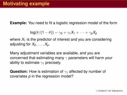
Example: You need to fit a logistic regression model of the form

log(/(1 )) = 0 + 1X1 + + pXpwhere X1 is the predictor of interest and you are consideringadjusting for X2, . . . ,Xp.

Many adjustment variables are available, and you areconcerned that estimating many parameters will harm yourability to estimate 1 precisely.

Question: How is estimation of 1 affected by number ofcovariates p in the regression model?

Motivating example

No obvious theoretical results to rely on (solves specialcase only or does not apply)

Solution? Simulate!

What is a simulation study?

A simulation study is a computer experiment, usuallyconducted by Monte Carlo (random) sampling from probabilitydistributions.

Two key features:

1 You control the truth! can explore many possible truthscenarios.

2 Computers dont get bored! can repeat experimentthousands of times to learn about sampling distribution ofparameters of interest.

Simulation study steps

1 Decide what quantities/properties you want to investigate2 Decide what truth scenarios you want to consider3 Write and optimize computer code for running simulations4 RUN simulations!... get a coffee... or two...5 Collect and summarize results6 Document the process

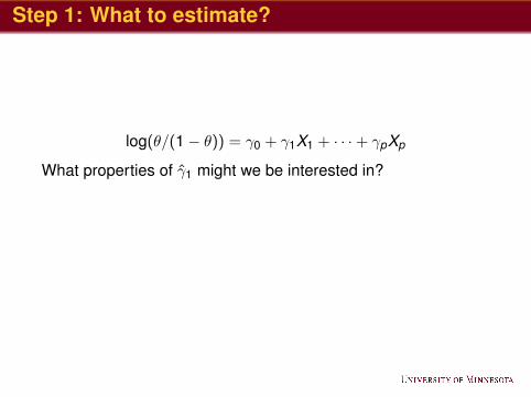
Step 1: What to estimate?

log(/(1 )) = 0 + 1X1 + + pXpWhat properties of 1 might we be interested in?

Bias Variance Confidence interval coverage Size/power of hypothesis tests

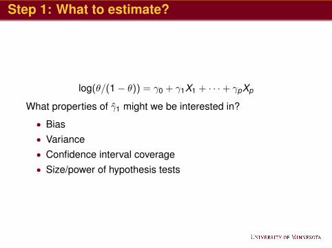
Step 1: What to estimate?

log(/(1 )) = 0 + 1X1 + + pXpWhat properties of 1 might we be interested in?

Bias Variance Confidence interval coverage Size/power of hypothesis tests

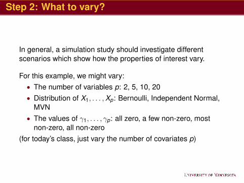
Step 2: What to vary?

In general, a simulation study should investigate differentscenarios which show how the properties of interest vary.

For this example, we might vary: The number of variables p: 2, 5, 10, 20 Distribution of X1, . . . ,Xp: Bernoulli, Independent Normal,

MVN The values of 1, . . . , p: all zero, a few non-zero, most

non-zero, all non-zero(for todays class, just vary the number of covariates p)

Step 3: Write and optimize computer code

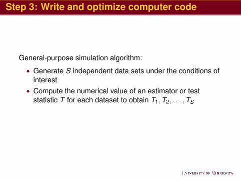
General-purpose simulation algorithm:

Generate S independent data sets under the conditions ofinterest

Compute the numerical value of an estimator or teststatistic T for each dataset to obtain T1,T2, . . . ,TS

Compute a summary statistic (e.g. mean, median) fromT1,T2, . . . ,TS to estimate properties of quantity of interest.

Step 3: Write and optimize computer code

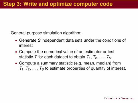
General-purpose simulation algorithm:

Generate S independent data sets under the conditions ofinterest

Compute the numerical value of an estimator or teststatistic T for each dataset to obtain T1,T2, . . . ,TS

Compute a summary statistic (e.g. mean, median) fromT1,T2, . . . ,TS to estimate properties of quantity of interest.

Step 3: Write and optimize computer code

General-purpose simulation algorithm:

Generate S independent data sets under the conditions ofinterest

Compute the numerical value of an estimator or teststatistic T for each dataset to obtain T1,T2, . . . ,TS

Compute a summary statistic (e.g. mean, median) fromT1,T2, . . . ,TS to estimate properties of quantity of interest.

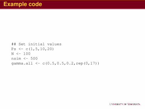
Example code

## Set initial valuesPs

Example code

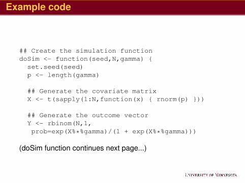
## Create the simulation functiondoSim

Example code

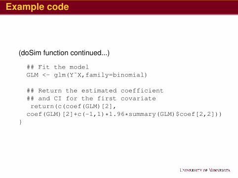
(doSim function continued...)

## Fit the modelGLM

Example code

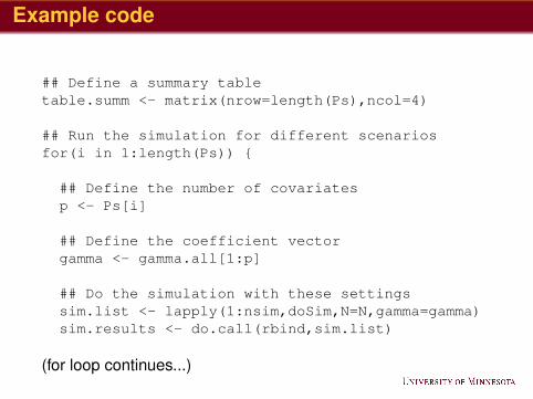
## Define a summary tabletable.summ

Example code

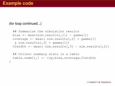
(for loop continued...)

## Summarize the simulation resultsbias

Big simulations

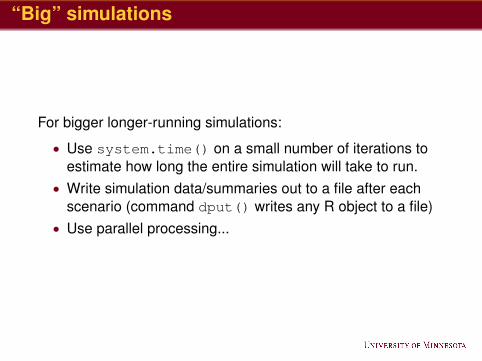
For bigger longer-running simulations:

Use system.time() on a small number of iterations toestimate how long the entire simulation will take to run.

Write simulation data/summaries out to a file after eachscenario (command dput() writes any R object to a file)

Use parallel processing...

Parallelization

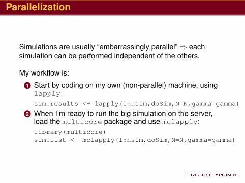
Simulations are usually embarrassingly parallel eachsimulation can be performed independent of the others.

My workflow is:

1 Start by coding on my own (non-parallel) machine, usinglapply:sim.results

Reproducibility

Simulations depend on random numbers and manyparameters and assumptions.

You may need to duplicate/reproduce your results, oftenmany months after code is first written!

Code may become part of an R package, or be madepublic as part of publication process.

For all these reasons, it is important to keep the idea ofreproducibility in mind when performing simulations.

Here are some tips...

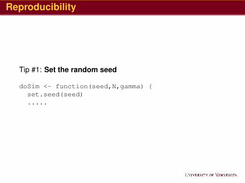
Reproducibility

Tip #1: Set the random seed

doSim

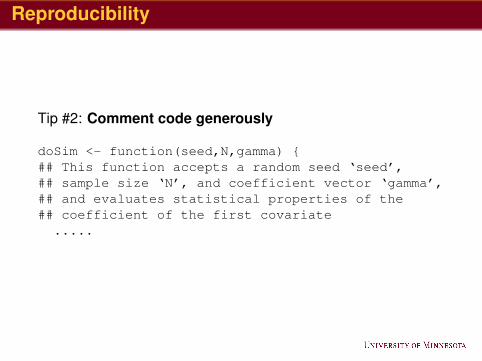
Reproducibility

Tip #2: Comment code generously

doSim

Reproducibility

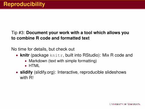
Tip #3: Document your work with a tool which allows youto combine R code and formatted text

No time for details, but check out knitr (package knitr, built into RStudio): Mix R code and

Markdown (text with simple formatting) HTML

slidify (slidify.org): Interactive, reproducible slideshowswith R!

Reproduciblity

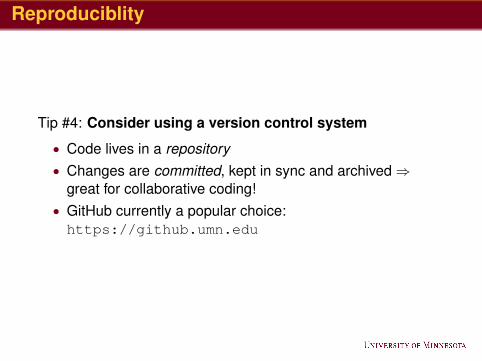
Tip #4: Consider using a version control system

Code lives in a repository Changes are committed, kept in sync and archived

great for collaborative coding! GitHub currently a popular choice:https://github.umn.edu

https://github.umn.edu

Presenting simulation results

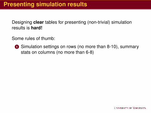
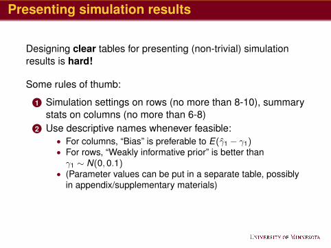
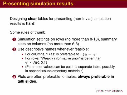
Designing clear tables for presenting (non-trivial) simulationresults is hard!

Some rules of thumb:

1 Simulation settings on rows (no more than 8-10), summarystats on columns (no more than 6-8)

2 Use descriptive names whenever feasible: For columns, Bias is preferable to E(1 1) For rows, Weakly informative prior is better than1 N(0,0.1)

(Parameter values can be put in a separate table, possiblyin appendix/supplementary materials)

3 Plots are often preferable to tables, always preferable intalk slides.

Presenting simulation results

Designing clear tables for presenting (non-trivial) simulationresults is hard!

Some rules of thumb:

1 Simulation settings on rows (no more than 8-10), summarystats on columns (no more than 6-8)

2 Use descriptive names whenever feasible: For columns, Bias is preferable to E(1 1) For rows, Weakly informative prior is better than1 N(0,0.1)

(Parameter values can be put in a separate table, possiblyin appendix/supplementary materials)

3 Plots are often preferable to tables, always preferable intalk slides.

Presenting simulation results

Designing clear tables for presenting (non-trivial) simulationresults is hard!

Some rules of thumb:

1 Simulation settings on rows (no more than 8-10), summarystats on columns (no more than 6-8)

2 Use descriptive names whenever feasible: For columns, Bias is preferable to E(1 1) For rows, Weakly informative prior is better than1 N(0,0.1)

(Parameter values can be put in a separate table, possiblyin appendix/supplementary materials)

3 Plots are often preferable to tables, always preferable intalk slides.

Presenting simulation results

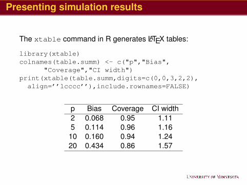
The xtable command in R generates LATEX tables:

library(xtable)colnames(table.summ)

Dealing with failure(s)

Sometimes, simulations will fail (p n regressionscenarios, survival data with no failures if failure is rare,etc.).

Specify in advance how you will handle iterations that fail,and keep track of proportion of failed iterations.

If failures are relatively uncommon (say 5%), caneliminate them from summary statistics and note that youhave done so.

Otherwise, reasons for failure should be carefullyinvestigated.

How many simulations do you need?

Can perform sample size calculation to see how manyyou need for desired precision (see Burton et al. (2006) oncourse web page).

But often, in practice... as many as you can do before themanuscript has to be submitted/revised!

In summary

Think about your simulation design before you startcoding.

Code efficiently to avoid unnecessary computation. Test your simulation on a small problem (or with a small

number of simulations) before running a larger one. Check for coding or possible algorithmic errors. Estimate how long the large simulation will take to run.

Save your results to disk frequently during the simulation;you dont want to lose several days/weeks of simulationsbecause of one failed iteration.

Summarize your results clearly and succinctly.

In summary

Think about your simulation design before you startcoding.

Code efficiently to avoid unnecessary computation.

Test your simulation on a small problem (or with a smallnumber of simulations) before running a larger one.

Check for coding or possible algorithmic errors. Estimate how long the large simulation will take to run.

Save your results to disk frequently during the simulation;you dont want to lose several days/weeks of simulationsbecause of one failed iteration.

Summarize your results clearly and succinctly.

In summary

Think about your simulation design before you startcoding.

Code efficiently to avoid unnecessary computation. Test your simulation on a small problem (or with a small

number of simulations) before running a larger one. Check for coding or possible algorithmic errors. Estimate how long the large simulation will take to run.

Save your results to disk frequently during the simulation;you dont want to lose several days/weeks of simulationsbecause of one failed iteration.

Summarize your results clearly and succinctly.

In summary

Think about your simulation design before you startcoding.

Code efficiently to avoid unnecessary computation. Test your simulation on a small problem (or with a small

number of simulations) before running a larger one. Check for coding or possible algorithmic errors. Estimate how long the large simulation will take to run.

Save your results to disk frequently during the simulation;you dont want to lose several days/weeks of simulationsbecause of one failed iteration.

Summarize your results clearly and succinctly.

In summary

Think about your simulation design before you startcoding.

Code efficiently to avoid unnecessary computation. Test your simulation on a small problem (or with a small

number of simulations) before running a larger one. Check for coding or possible algorithmic errors. Estimate how long the large simulation will take to run.

Save your results to disk frequently during the simulation;you dont want to lose several days/weeks of simulationsbecause of one failed iteration.

Summarize your results clearly and succinctly.

Assignment

Conduct a simple simulation study and summarize the resultsin a short ( 1 page, Word, LATEX or knitr/Markdown generatedPDF!). You may either select your own topic, or use one of thetopics provided on the following pages.

Assignments should be turned in one week from today, i.e. onSeptember 17.

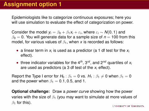
Assignment option 1

Epidemiologists like to categorize continuous exposures; here youwill use simulation to evaluate the effect of categorization on power.

Consider the model yi = 0 + 1xi + i , where i N(0,1) and0 = 0. You will generate data for a sample size of n = 100 from thismodel, for various values of 1, when x is recorded as follows:

a linear term in xi is used as a predictor (a 1 df test for the xieffect).

three indicator variables for the 4th, 3rd , and 2nd quartiles of xiare used as predictors (a 3 df test of the xi effect).

Report the Type I error for H0 : 1 = 0 vs. H1 : 1 6= 0 when 1 = 0and the power when 1 = 0.1,0.5, and 1.

Optional challenge: Draw a power curve showing how the powervaries with the size of 1 (you may want to simulate at more values of1 for this).

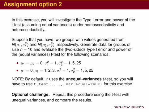
Assignment option 2

In this exercise, you will investigate the Type I error and power of thet-test (assuming equal variances) under homoscedasticity andheteroscedasticity.

Suppose that you have two groups with values generated fromN(1, 21) and N(2,

22), respectively. Generate data for groups of

size n = 10 and evaluate the (two-sided) Type I error and power ofthe (equal variances) t-test for the following scenarios:

1 = 2 = 0, 21 = 1, 22 = 1,5,25

1 = 0, 2 = 1,2,3, 21 = 1, 22 = 1,5,25

NOTE: By default, R uses the unequal-variances t-test, so you willhave to use t.test(...., var.equal=TRUE) for this exercise.

Optional challenge: Repeat this procedure using the t-test withunequal variances, and compare the results.