Pseudospektren f¨ur strukturierte Matrixst¨orungen Michael ...... Basic question: How do the...
64
Pseudospektren f¨ ur strukturierte Matrixst¨orungen Michael Karow Matheon, TU-Berlin
Transcript of Pseudospektren f¨ur strukturierte Matrixst¨orungen Michael ...... Basic question: How do the...
Pseudospektren fur strukturierte
Matrixstorungen
Michael Karow
Matheon, TU-Berlin
Eigenvalue perturbation theory.
An approach via pseudospectra and µ-functions
Michael Karow
Matheon, TU-Berlin

Motivation.
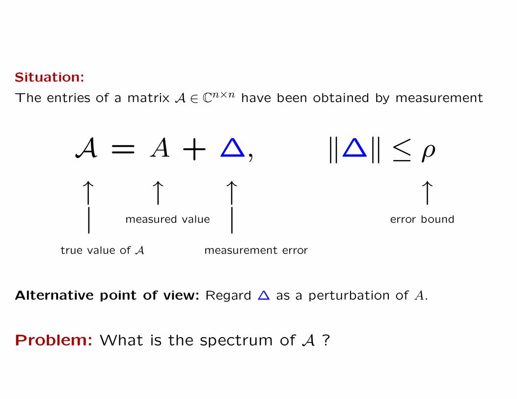
Situation:
The entries of a matrix A ∈ Cn×n have been obtained by measurement
A = A + ∆, ‖∆‖ ≤ ρ
↑ ↑ ↑ ↑| |measured value error bound
true value of A measurement error
Alternative point of view: Regard ∆ as a perturbation of A.
Problem: What is the spectrum of A ?
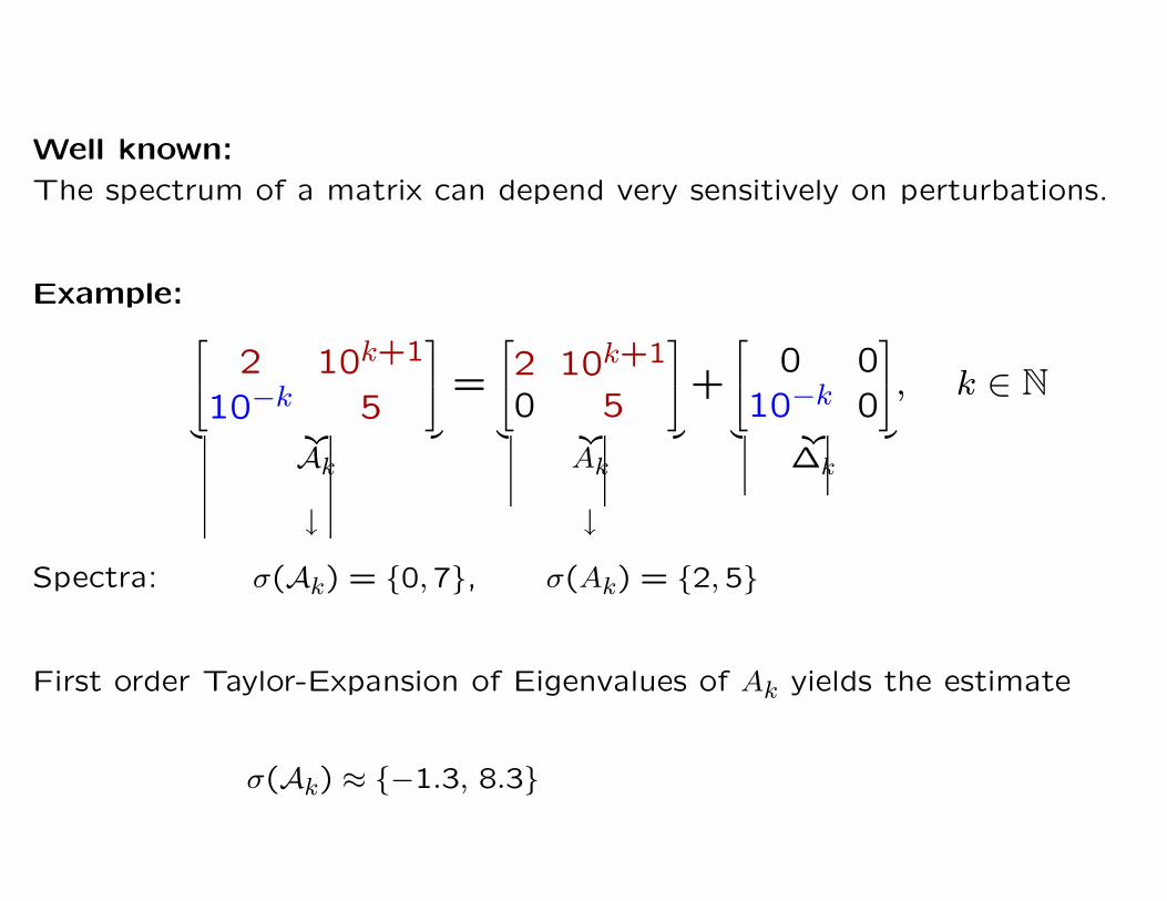
Well known:
The spectrum of a matrix can depend very sensitively on perturbations.
Example:
2 10k+1
10−k 5
︸ ︷︷ ︸Ak
=
2 10k+1
0 5
︸ ︷︷ ︸Ak
+
0 0
10−k 0
︸ ︷︷ ︸∆k
, k ∈ N
↓ ↓
Spectra: σ(Ak) = {0,7}, σ(Ak) = {2,5}
First order Taylor-Expansion of Eigenvalues of Ak yields the estimate
σ(Ak) ≈ {−1.3, 8.3}

The framework.
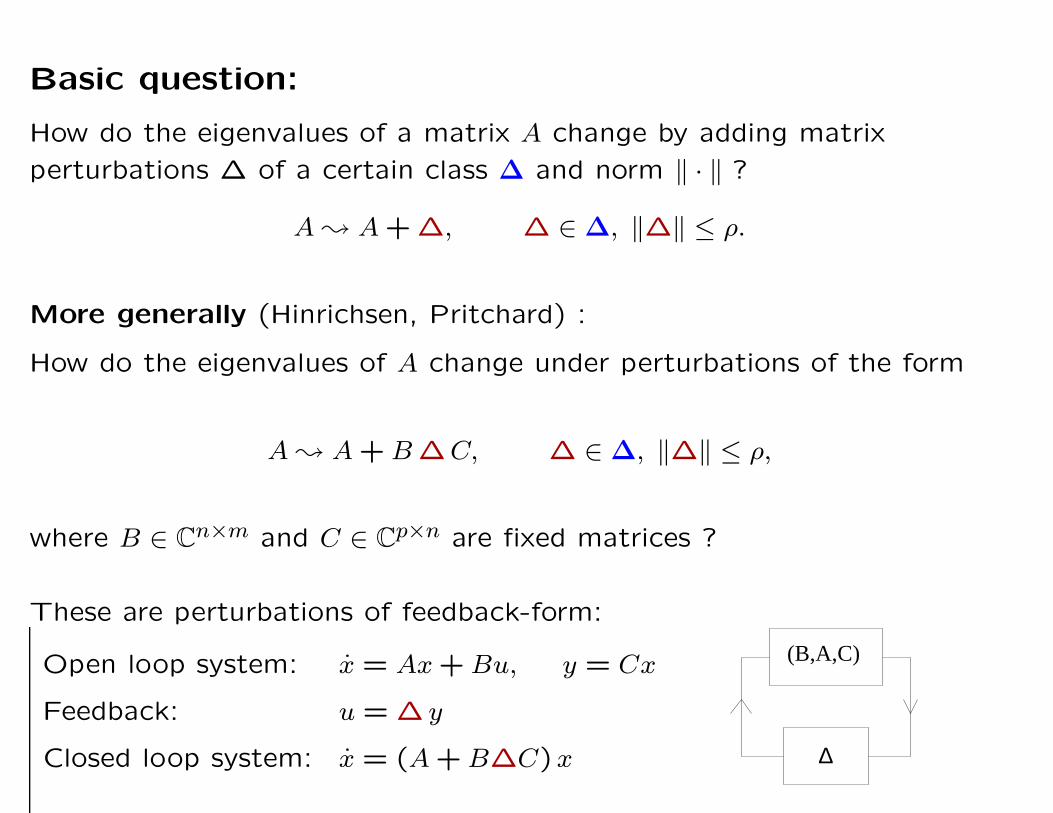
Basic question:
How do the eigenvalues of a matrix A change by adding matrix
perturbations ∆ of a certain class ∆ and norm ‖ · ‖ ?
A ; A + ∆, ∆ ∈ ∆, ‖∆‖ ≤ ρ.
More generally (Hinrichsen, Pritchard) :
How do the eigenvalues of A change under perturbations of the form
A ; A + B ∆C, ∆ ∈ ∆, ‖∆‖ ≤ ρ,
where B ∈ Cn×m and C ∈ Cp×n are fixed matrices ?
These are perturbations of feedback-form:
Open loop system: x = Ax + Bu, y = Cx
Feedback: u = ∆ y
Closed loop system: x = (A + B∆C)x ∆
(B,A,C)
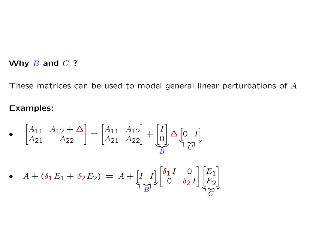
Why B and C ?
These matrices can be used to model general linear perturbations of A
Examples:
•[A11 A12 + ∆A21 A22
]=
[A11 A12A21 A22
]+
[I0
]
︸︷︷︸B
∆[0 I
]
︸ ︷︷ ︸C
• A + (δ1 E1 + δ2 E2) = A +[I I
]
︸ ︷︷ ︸B
[δ1 I 00 δ2 I
] [E1E2
]
︸ ︷︷ ︸C
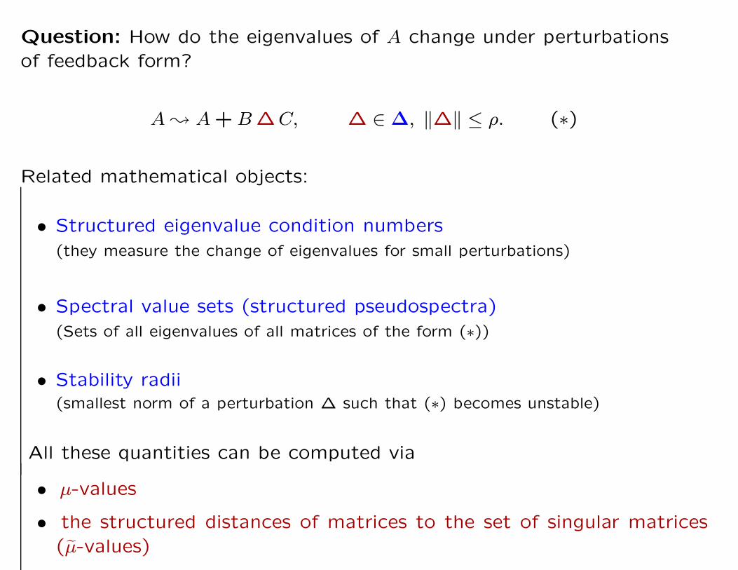
Question: How do the eigenvalues of A change under perturbations
of feedback form?
A ; A + B ∆C, ∆ ∈ ∆, ‖∆‖ ≤ ρ. (∗)
Related mathematical objects:
• Structured eigenvalue condition numbers
(they measure the change of eigenvalues for small perturbations)
• Spectral value sets (structured pseudospectra)
(Sets of all eigenvalues of all matrices of the form (∗))
• Stability radii
(smallest norm of a perturbation ∆ such that (∗) becomes unstable)
All these quantities can be computed via
• µ-values
• the structured distances of matrices to the set of singular matrices
(µ-values)
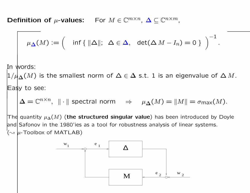
Definition of µ-values: For M ∈ Cm×n, ∆ ⊆ Cn×m,
µ∆(M) :=
(inf { ‖∆‖; ∆ ∈ ∆, det(∆M − In) = 0 }
)−1
.
In words:
1/µ∆(M) is the smallest norm of ∆ ∈ ∆ s.t. 1 is an eigenvalue of ∆M .
Easy to see:
∆ = Cn×n, ‖ · ‖ spectral norm ⇒ µ∆(M) = ‖M‖ = σmax(M).
The quantity µ∆(M) (the structured singular value) has been introduced by Doyle
and Safonov in the 1980’ies as a tool for robustness analysis of linear systems.
(; µ-Toolbox of MATLAB)
e w
w1 1
e
22
∆
M
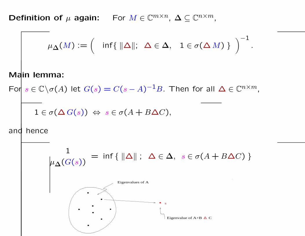
Definition of µ again: For M ∈ Cm×n, ∆ ⊆ Cn×m,
µ∆(M) :=
(inf{ ‖∆‖; ∆ ∈ ∆, 1 ∈ σ(∆M) }
)−1
.
Main lemma:
For s ∈ C\σ(A) let G(s) = C(s − A)−1B. Then for all ∆ ∈ Cn×m,
1 ∈ σ(∆G(s)) ⇔ s ∈ σ(A + B∆C),
and hence
1
µ∆(G(s))= inf { ‖∆‖ ; ∆ ∈ ∆, s ∈ σ(A + B∆C) }
s
Eigenvalues of A
Eigenvalue of A+B C∆
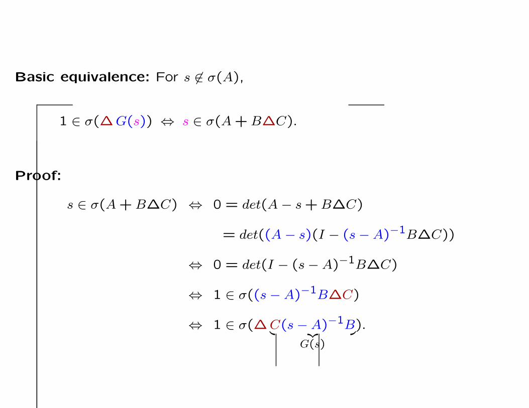
Basic equivalence: For s 6∈ σ(A),
1 ∈ σ(∆G(s)) ⇔ s ∈ σ(A + B∆C).
Proof:
s ∈ σ(A + B∆C) ⇔ 0 = det(A − s + B∆C)
= det((A − s)(I − (s − A)−1B∆C))
⇔ 0 = det(I − (s − A)−1B∆C)
⇔ 1 ∈ σ((s − A)−1B∆C)
⇔ 1 ∈ σ(∆C(s − A)−1B︸ ︷︷ ︸G(s)
).
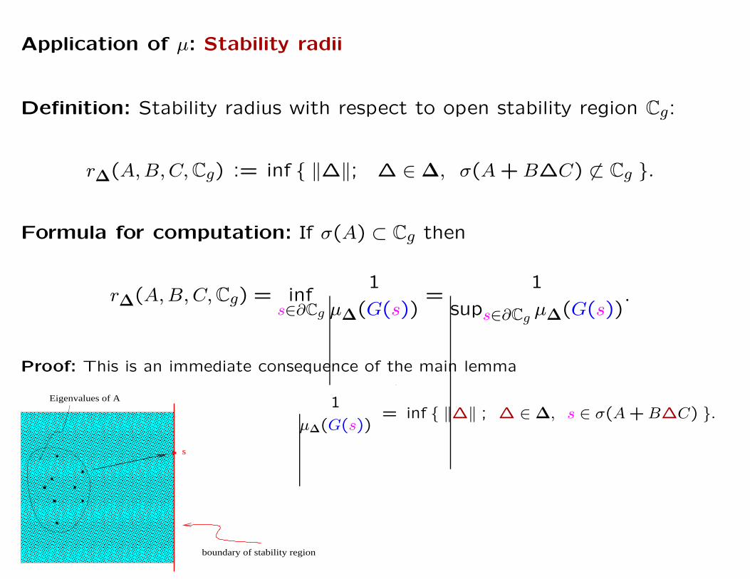
Application of µ: Stability radii
Definition: Stability radius with respect to open stability region Cg:
r∆(A, B, C, Cg) := inf { ‖∆‖; ∆ ∈ ∆, σ(A + B∆C) 6⊂ Cg }.
Formula for computation: If σ(A) ⊂ Cg then
r∆(A, B, C, Cg) = infs∈∂Cg
1
µ∆(G(s))=
1
sups∈∂Cgµ∆(G(s))
.
Proof: This is an immediate consequence of the main lemma
1
µ∆(G(s))= inf { ‖∆‖ ; ∆ ∈ ∆, s ∈ σ(A + B∆C) }.
� � � � � � � � � � � � � � � � � � �� � � � � � � � � � � � � � � � � � �� � � � � � � � � � � � � � � � � � �� � � � � � � � � � � � � � � � � � �� � � � � � � � � � � � � � � � � � �� � � � � � � � � � � � � � � � � � �� � � � � � � � � � � � � � � � � � �� � � � � � � � � � � � � � � � � � �� � � � � � � � � � � � � � � � � � �� � � � � � � � � � � � � � � � � � �� � � � � � � � � � � � � � � � � � �� � � � � � � � � � � � � � � � � � �� � � � � � � � � � � � � � � � � � �� � � � � � � � � � � � � � � � � � �� � � � � � � � � � � � � � � � � � �� � � � � � � � � � � � � � � � � � �� � � � � � � � � � � � � � � � � � �� � � � � � � � � � � � � � � � � � �� � � � � � � � � � � � � � � � � � �� � � � � � � � � � � � � � � � � � �� � � � � � � � � � � � � � � � � � �� � � � � � � � � � � � � � � � � � �� � � � � � � � � � � � � � � � � � �� � � � � � � � � � � � � � � � � � �� � � � � � � � � � � � � � � � � � �� � � � � � � � � � � � � � � � � � �� � � � � � � � � � � � � � � � � � �� � � � � � � � � � � � � � � � � � �� � � � � � � � � � � � � � � � � � �� � � � � � � � � � � � � � � � � � �� � � � � � � � � � � � � � � � � � �� � � � � � � � � � � � � � � � � � �� � � � � � � � � � � � � � � � � � �� � � � � � � � � � � � � � � � � � �� � � � � � � � � � � � � � � � � � �� � � � � � � � � � � � � � � � � � �� � � � � � � � � � � � � � � � � � �� � � � � � � � � � � � � � � � � � �� � � � � � � � � � � � � � � � � � �� � � � � � � � � � � � � � � � � � �� � � � � � � � � � � � � � � � � � �� � � � � � � � � � � � � � � � � � �� � � � � � � � � � � � � � � � � � �
� � � � � � � � � � � � � � � � � � �� � � � � � � � � � � � � � � � � � �� � � � � � � � � � � � � � � � � � �� � � � � � � � � � � � � � � � � � �� � � � � � � � � � � � � � � � � � �� � � � � � � � � � � � � � � � � � �� � � � � � � � � � � � � � � � � � �� � � � � � � � � � � � � � � � � � �� � � � � � � � � � � � � � � � � � �� � � � � � � � � � � � � � � � � � �� � � � � � � � � � � � � � � � � � �� � � � � � � � � � � � � � � � � � �� � � � � � � � � � � � � � � � � � �� � � � � � � � � � � � � � � � � � �� � � � � � � � � � � � � � � � � � �� � � � � � � � � � � � � � � � � � �� � � � � � � � � � � � � � � � � � �� � � � � � � � � � � � � � � � � � �� � � � � � � � � � � � � � � � � � �� � � � � � � � � � � � � � � � � � �� � � � � � � � � � � � � � � � � � �� � � � � � � � � � � � � � � � � � �� � � � � � � � � � � � � � � � � � �� � � � � � � � � � � � � � � � � � �� � � � � � � � � � � � � � � � � � �� � � � � � � � � � � � � � � � � � �� � � � � � � � � � � � � � � � � � �� � � � � � � � � � � � � � � � � � �� � � � � � � � � � � � � � � � � � �� � � � � � � � � � � � � � � � � � �� � � � � � � � � � � � � � � � � � �� � � � � � � � � � � � � � � � � � �� � � � � � � � � � � � � � � � � � �� � � � � � � � � � � � � � � � � � �� � � � � � � � � � � � � � � � � � �� � � � � � � � � � � � � � � � � � �� � � � � � � � � � � � � � � � � � �� � � � � � � � � � � � � � � � � � �� � � � � � � � � � � � � � � � � � �� � � � � � � � � � � � � � � � � � �� � � � � � � � � � � � � � � � � � �� � � � � � � � � � � � � � � � � � �� � � � � � � � � � � � � � � � � � �
s
Eigenvalues of A
boundary of stability region
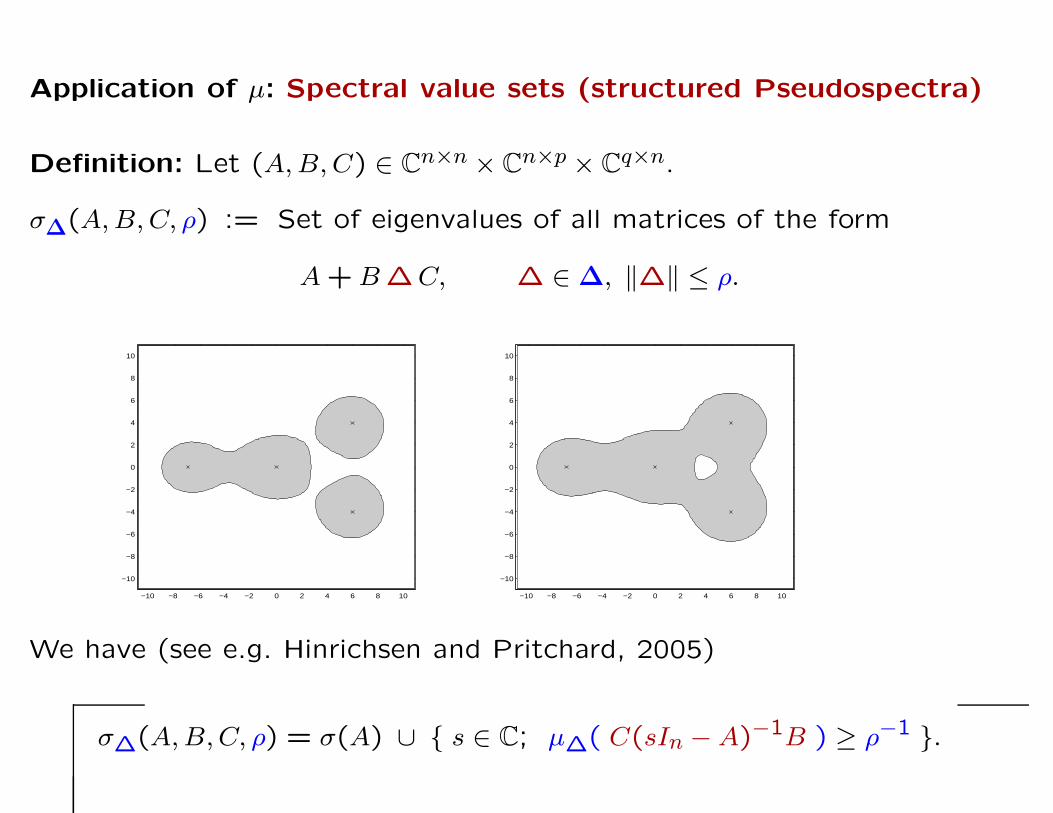
Application of µ: Spectral value sets (structured Pseudospectra)
Definition: Let (A, B, C) ∈ Cn×n × Cn×p × Cq×n.
σ∆(A, B, C, ρ) := Set of eigenvalues of all matrices of the form
A + B ∆C, ∆ ∈ ∆, ‖∆‖ ≤ ρ.
−10 −8 −6 −4 −2 0 2 4 6 8 10
−10
−8
−6
−4
−2
0
2
4
6
8
10
−10 −8 −6 −4 −2 0 2 4 6 8 10
−10
−8
−6
−4
−2
0
2
4
6
8
10
We have (see e.g. Hinrichsen and Pritchard, 2005)
σ∆(A, B, C, ρ) = σ(A) ∪ { s ∈ C; µ∆( C(sIn − A)−1B ) ≥ ρ−1 }.
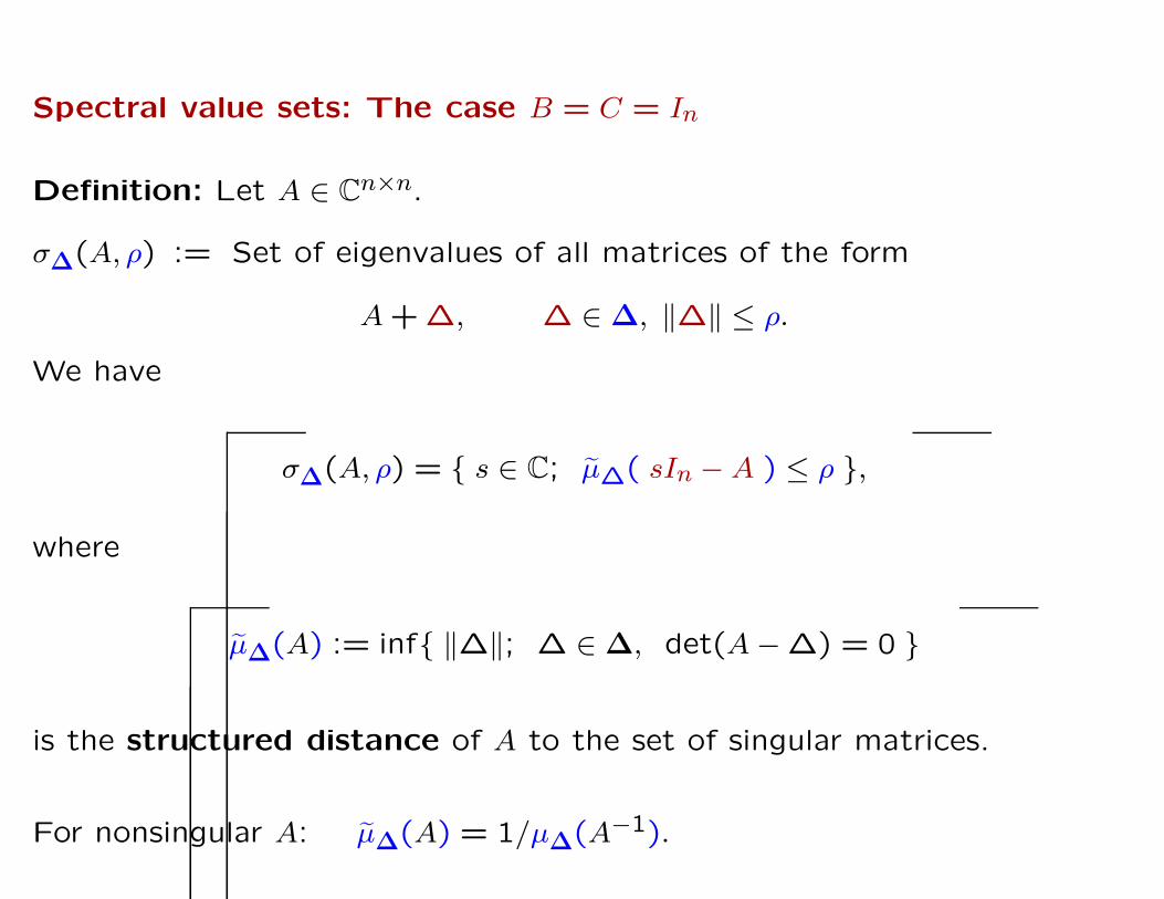
Spectral value sets: The case B = C = In
Definition: Let A ∈ Cn×n.
σ∆(A, ρ) := Set of eigenvalues of all matrices of the form
A + ∆, ∆ ∈ ∆, ‖∆‖ ≤ ρ.
We have
σ∆(A, ρ) = { s ∈ C; µ∆( sIn − A ) ≤ ρ },
where
µ∆(A) := inf{ ‖∆‖; ∆ ∈ ∆, det(A − ∆) = 0 }
is the structured distance of A to the set of singular matrices.
For nonsingular A: µ∆(A) = 1/µ∆(A−1).
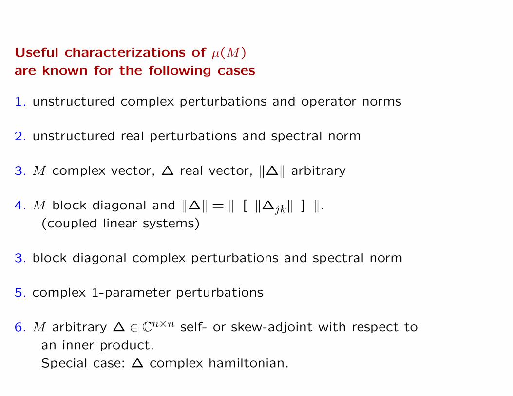
Useful characterizations of µ(M)
are known for the following cases
1. unstructured complex perturbations and operator norms
2. unstructured real perturbations and spectral norm
3. M complex vector, ∆ real vector, ‖∆‖ arbitrary
4. M block diagonal and ‖∆‖ = ‖ [ ‖∆jk‖ ] ‖.(coupled linear systems)
3. block diagonal complex perturbations and spectral norm
5. complex 1-parameter perturbations
6. M arbitrary ∆ ∈ Cn×n self- or skew-adjoint with respect to
an inner product.
Special case: ∆ complex hamiltonian.
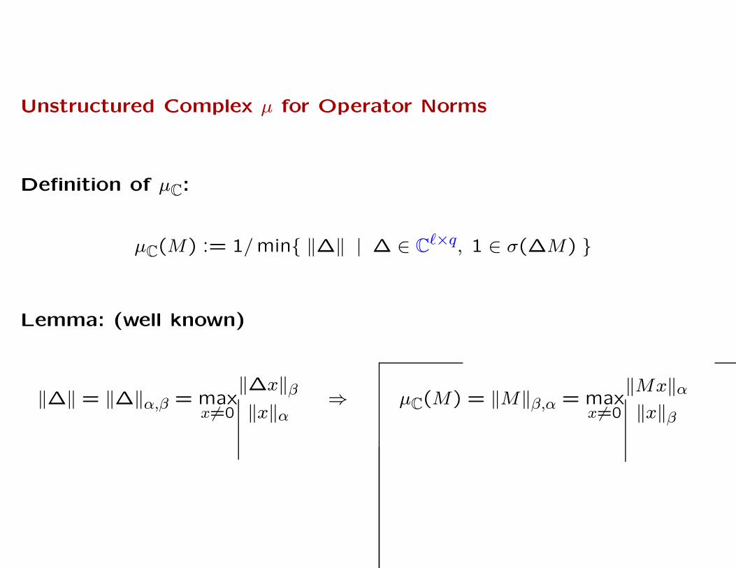
Unstructured Complex µ for Operator Norms
Definition of µC:
µC(M) := 1/min{ ‖∆‖ | ∆ ∈ C`×q, 1 ∈ σ(∆M) }
Lemma: (well known)
‖∆‖ = ‖∆‖α,β = maxx6=0
‖∆x‖β
‖x‖α⇒ µC(M) = ‖M‖β,α = max
x6=0
‖Mx‖α
‖x‖β

Real Perturbations.
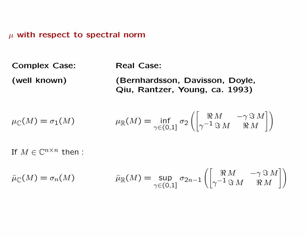
µ with respect to spectral norm
Complex Case: Real Case:
(well known) (Bernhardsson, Davisson, Doyle,Qiu, Rantzer, Young, ca. 1993)
µC(M) = σ1(M) µR(M) = infγ∈(0,1]
σ2
([<M −γ =M
γ−1=M <M
])
If M ∈ Cn×n then :
µC(M) = σn(M) µR(M) = supγ∈(0,1]
σ2n−1
([<M −γ =M
γ−1=M <M
])
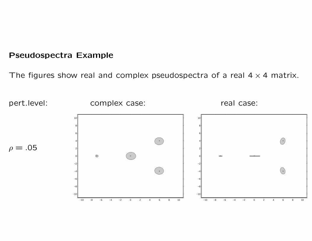
Pseudospectra Example
The figures show real and complex pseudospectra of a real 4× 4 matrix.
pert.level: complex case: real case:
ρ = .05
−10 −8 −6 −4 −2 0 2 4 6 8 10
−10
−8
−6
−4
−2
0
2
4
6
8
10
−10 −8 −6 −4 −2 0 2 4 6 8 10
−10
−8
−6
−4
−2
0
2
4
6
8
10
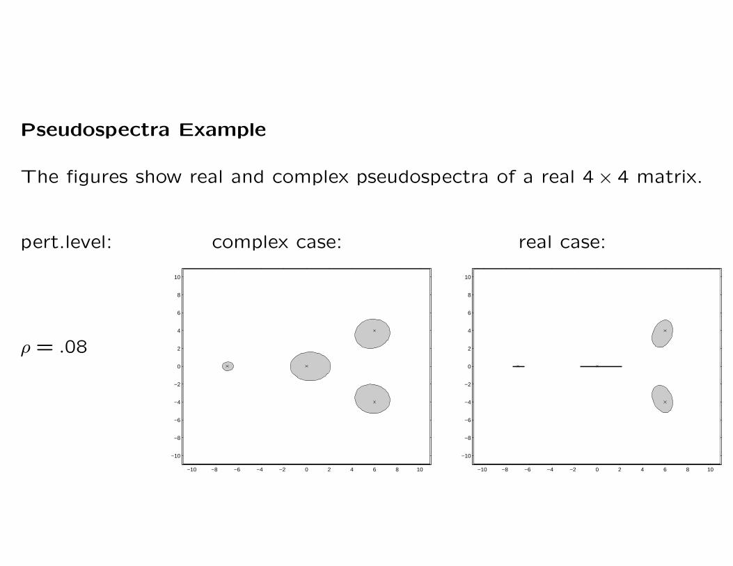
Pseudospectra Example
The figures show real and complex pseudospectra of a real 4× 4 matrix.
pert.level: complex case: real case:
ρ = .08
−10 −8 −6 −4 −2 0 2 4 6 8 10
−10
−8
−6
−4
−2
0
2
4
6
8
10
−10 −8 −6 −4 −2 0 2 4 6 8 10
−10
−8
−6
−4
−2
0
2
4
6
8
10
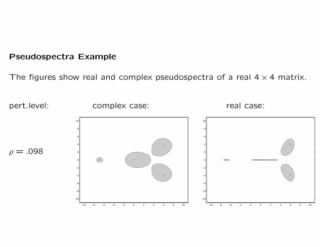
Pseudospectra Example
The figures show real and complex pseudospectra of a real 4× 4 matrix.
pert.level: complex case: real case:
ρ = .098
−10 −8 −6 −4 −2 0 2 4 6 8 10
−10
−8
−6
−4
−2
0
2
4
6
8
10
−10 −8 −6 −4 −2 0 2 4 6 8 10
−10
−8
−6
−4
−2
0
2
4
6
8
10

Pseudospectra Example
The figures show real and complex pseudospectra of a real 4× 4 matrix.
pert.level: complex case: real case:
ρ = .1
−10 −8 −6 −4 −2 0 2 4 6 8 10
−10
−8
−6
−4
−2
0
2
4
6
8
10
−10 −8 −6 −4 −2 0 2 4 6 8 10
−10
−8
−6
−4
−2
0
2
4
6
8
10
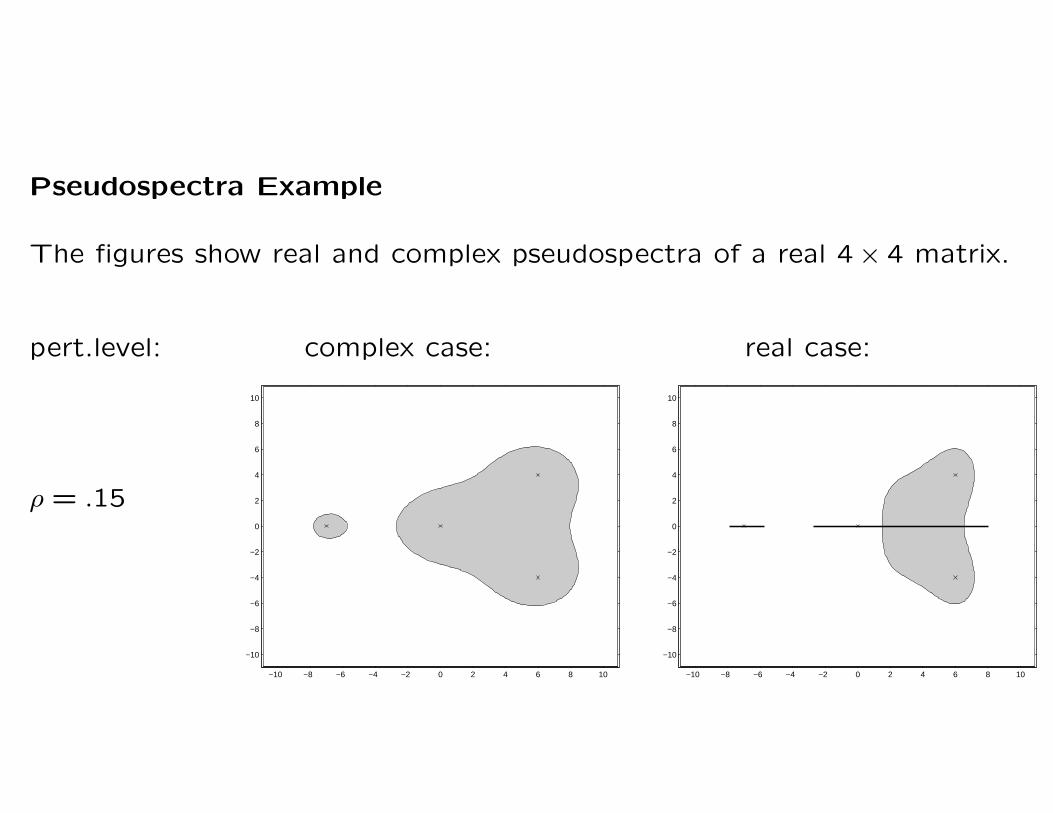
Pseudospectra Example
The figures show real and complex pseudospectra of a real 4× 4 matrix.
pert.level: complex case: real case:
ρ = .15
−10 −8 −6 −4 −2 0 2 4 6 8 10
−10
−8
−6
−4
−2
0
2
4
6
8
10
−10 −8 −6 −4 −2 0 2 4 6 8 10
−10
−8
−6
−4
−2
0
2
4
6
8
10
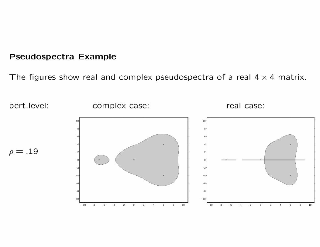
Pseudospectra Example
The figures show real and complex pseudospectra of a real 4× 4 matrix.
pert.level: complex case: real case:
ρ = .19
−10 −8 −6 −4 −2 0 2 4 6 8 10
−10
−8
−6
−4
−2
0
2
4
6
8
10
−10 −8 −6 −4 −2 0 2 4 6 8 10
−10
−8
−6
−4
−2
0
2
4
6
8
10

Pseudospectra Example
The figures show real and complex pseudospectra of a real 4× 4 matrix.
pert.level: complex case: real case:
ρ = .2
−10 −8 −6 −4 −2 0 2 4 6 8 10
−10
−8
−6
−4
−2
0
2
4
6
8
10
−10 −8 −6 −4 −2 0 2 4 6 8 10
−10
−8
−6
−4
−2
0
2
4
6
8
10
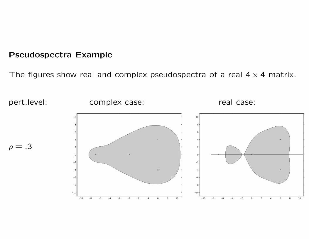
Pseudospectra Example
The figures show real and complex pseudospectra of a real 4× 4 matrix.
pert.level: complex case: real case:
ρ = .3
−10 −8 −6 −4 −2 0 2 4 6 8 10
−10
−8
−6
−4
−2
0
2
4
6
8
10
−10 −8 −6 −4 −2 0 2 4 6 8 10
−10
−8
−6
−4
−2
0
2
4
6
8
10
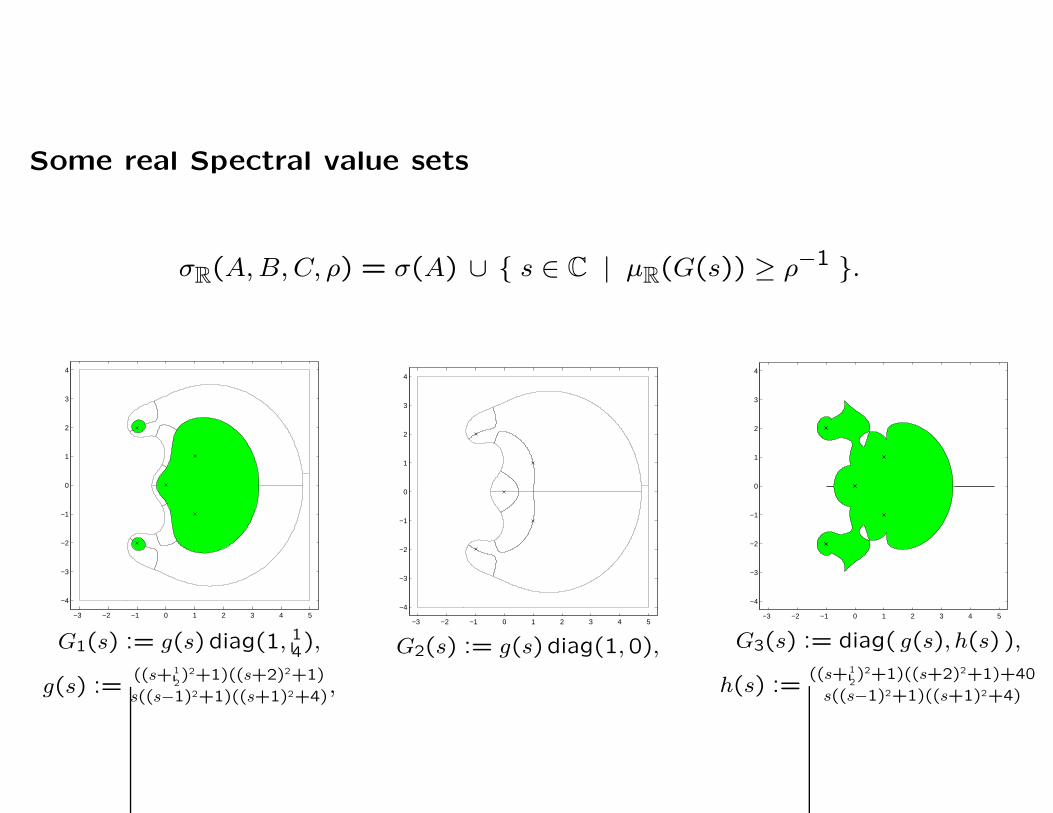
Some real Spectral value sets
σR(A, B, C, ρ) = σ(A) ∪ { s ∈ C | µR(G(s)) ≥ ρ−1 }.
−3 −2 −1 0 1 2 3 4 5
−4
−3
−2
−1
0
1
2
3
4
G1(s) := g(s) diag(1, 14),
g(s) :=((s+1
2)2+1)((s+2)2+1)
s((s−1)2+1)((s+1)2+4),
−3 −2 −1 0 1 2 3 4 5
−4
−3
−2
−1
0
1
2
3
4
G2(s) := g(s) diag(1,0),
−3 −2 −1 0 1 2 3 4 5
−4
−3
−2
−1
0
1
2
3
4
G3(s) := diag( g(s), h(s) ),
h(s) :=((s+1
2)2+1)((s+2)2+1)+40
s((s−1)2+1)((s+1)2+4)
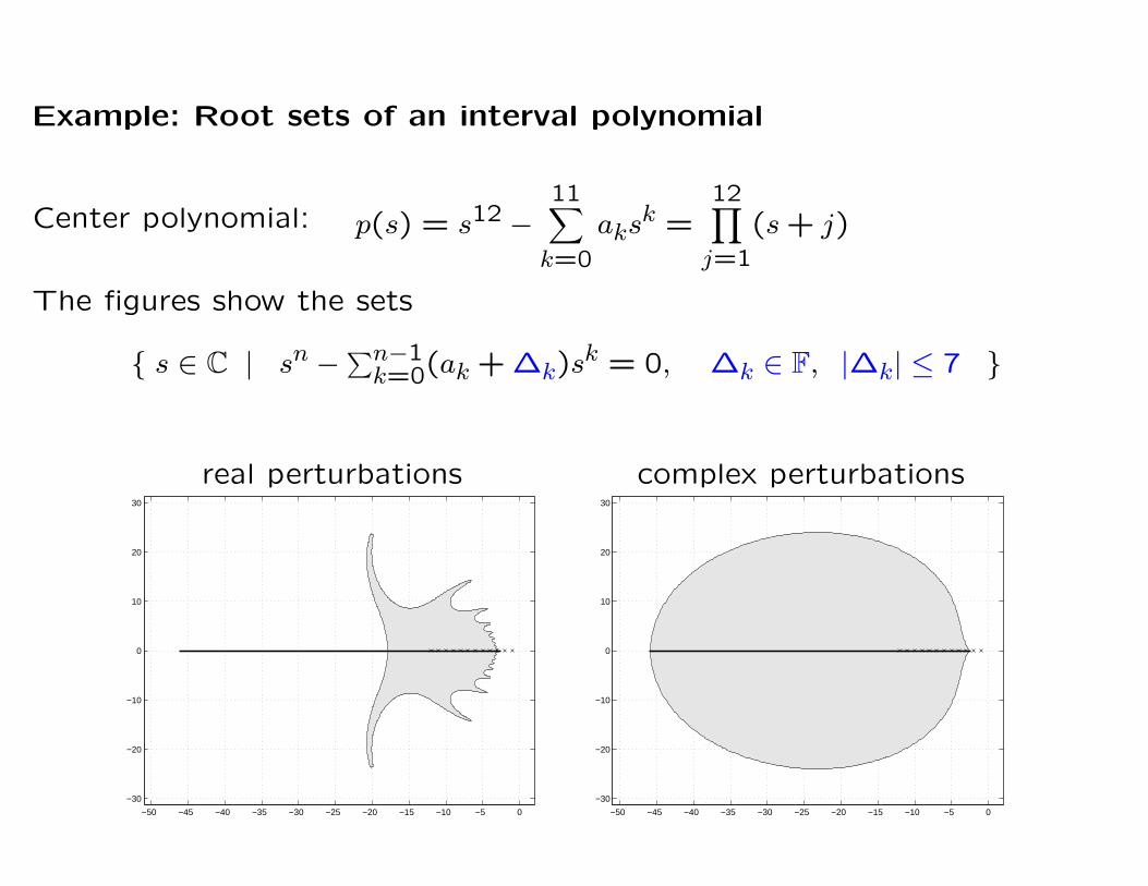
Example: Root sets of an interval polynomial
Center polynomial: p(s) = s12 −11∑
k=0
aksk =12∏
j=1
(s + j)
The figures show the sets
{ s ∈ C | sn −∑n−1k=0(ak + ∆k)s
k = 0, ∆k ∈ F, |∆k| ≤ 7 }
real perturbations complex perturbations
−50 −45 −40 −35 −30 −25 −20 −15 −10 −5 0
−30
−20
−10
0
10
20
30
−50 −45 −40 −35 −30 −25 −20 −15 −10 −5 0
−30
−20
−10
0
10
20
30

Hamiltonian Perturbations.

Definitions:
J-matrix: J =
[0 In
−In 0
]∈ C2n×2n
Fundamental property: J∗ = −J.
Set of complex ∗-Hamiltonian matrices:
Ham = {H ∈ C2n×2n; H∗J = −JH } (J-skew-adjoint matrices)
= {H ∈ C2n×2n; (JH)∗ = JH }
= { JH0 ∈ C2n×2n; H∗
0 = H0 }
=
{[A BC −A∗
]; B = B∗, C = C∗
}
Spectral symmetry:
The spectrum of a Hamiltonian matrix is
symmetric with respect to the imaginary axis:
λ ∈ σ(H) ⇒ −λ ∈ σ(H)� �
� �� �
� � �
� �
� �� �
� �� �
� � � � � � � � � � � � � � � � � � �
� � � � � � � � � � � � � � � � � � �
� � � � � � � � � � � � � � � � � � �
� � � � � � � � � � � � � � � � � � �
� � � � � � � � � � � � � � � � � � �
� � � � � � � � � � � � � � � � � � �
� � � � � � � � � � � � � � � � � � �
� � � � � � � � � � � � � � � � � � �
� � � � � � � � � � � � � � � � � � �
� � � � � � � � � � � � � � � � � � �
� � � � � � � � � � � � � � � � � � �
� � � � � � � � � � � � � � � � � � �
� � � � � � � � � � � � � � � � � � �
� � � � � � � � � � � � � � � � � � �
� � � � � � � � � � � � � � � � � � �
� � � � � � � � � � � � � � � � � � �
� � � � � � � � � � � � � � � � � � �
� � � � � � � � � � � � � � � � � � �
� � � � � � � � � � � � � � � � � � �
� � � � � � � � � � � � � � � � � � �
� � � � � � � � � � � � � � � � � � �
� � � � � � � � � � � � � � � � � � �
� � � � � � � � � � � � � � � � � � �
� � � � � � � � � � � � � � � � � � �
� � � � � � � � � � � � � � � � � � �
� � � � � � � � � � � � � � � � � � �
� � � � � � � � � � � � � � � � � � �
� � � � � � � � � � � � � � � � � � �
� � � � � � � � � � � � � � � � � � �
� � � � � � � � � � � � � � � � � � �
� � � � � � � � � � � � � � � � � � �
� � � � � � � � � � � � � � � � � � �
� � � � � � � � � � � � � � � � � � �
� � � � � � � � � � � � � � � � � � �
� � � � � � � � � � � � � � � � � � �
� � � � � � � � � � � � � � � � � � �
i α
λ λ
imaginary Axis
0
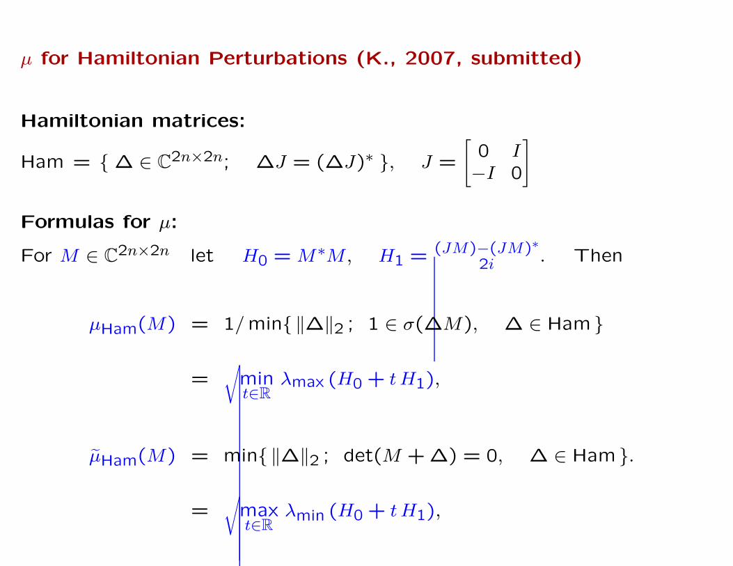
µ for Hamiltonian Perturbations (K., 2007, submitted)
Hamiltonian matrices:
Ham = { ∆ ∈ C2n×2n; ∆J = (∆J)∗ }, J =
[0 I−I 0
]
Formulas for µ:
For M ∈ C2n×2n let H0 = M∗M, H1 = (JM)−(JM)∗2i . Then
µHam(M) = 1/min{ ‖∆‖2 ; 1 ∈ σ(∆M), ∆ ∈ Ham }
=√
mint∈R
λmax (H0 + t H1),
µHam(M) = min{ ‖∆‖2 ; det(M + ∆) = 0, ∆ ∈ Ham }.
=√
maxt∈R
λmin (H0 + t H1),
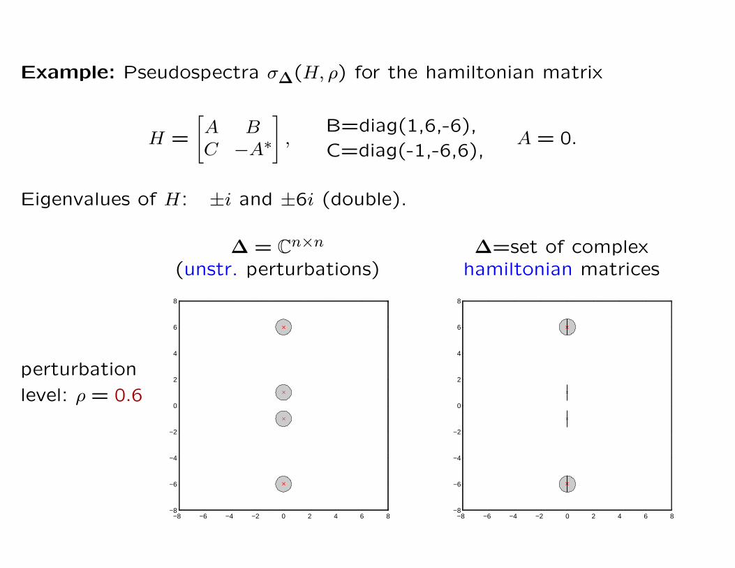
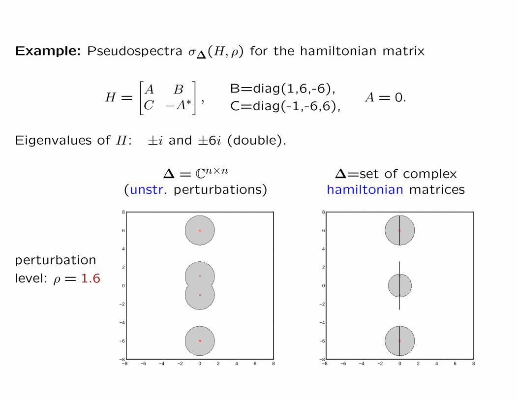
Example: Pseudospectra σ∆(H, ρ) for the hamiltonian matrix
H =
[A BC −A∗
],
B=diag(1,6,-6),
C=diag(-1,-6,6),A = 0.
Eigenvalues of H: ±i and ±6i (double).
∆ = Cn×n ∆=set of complex(unstr. perturbations) hamiltonian matrices
−8 −6 −4 −2 0 2 4 6 8−8
−6
−4
−2
0
2
4
6
8
−8 −6 −4 −2 0 2 4 6 8−8
−6
−4
−2
0
2
4
6
8
perturbation
level: ρ = 0.6
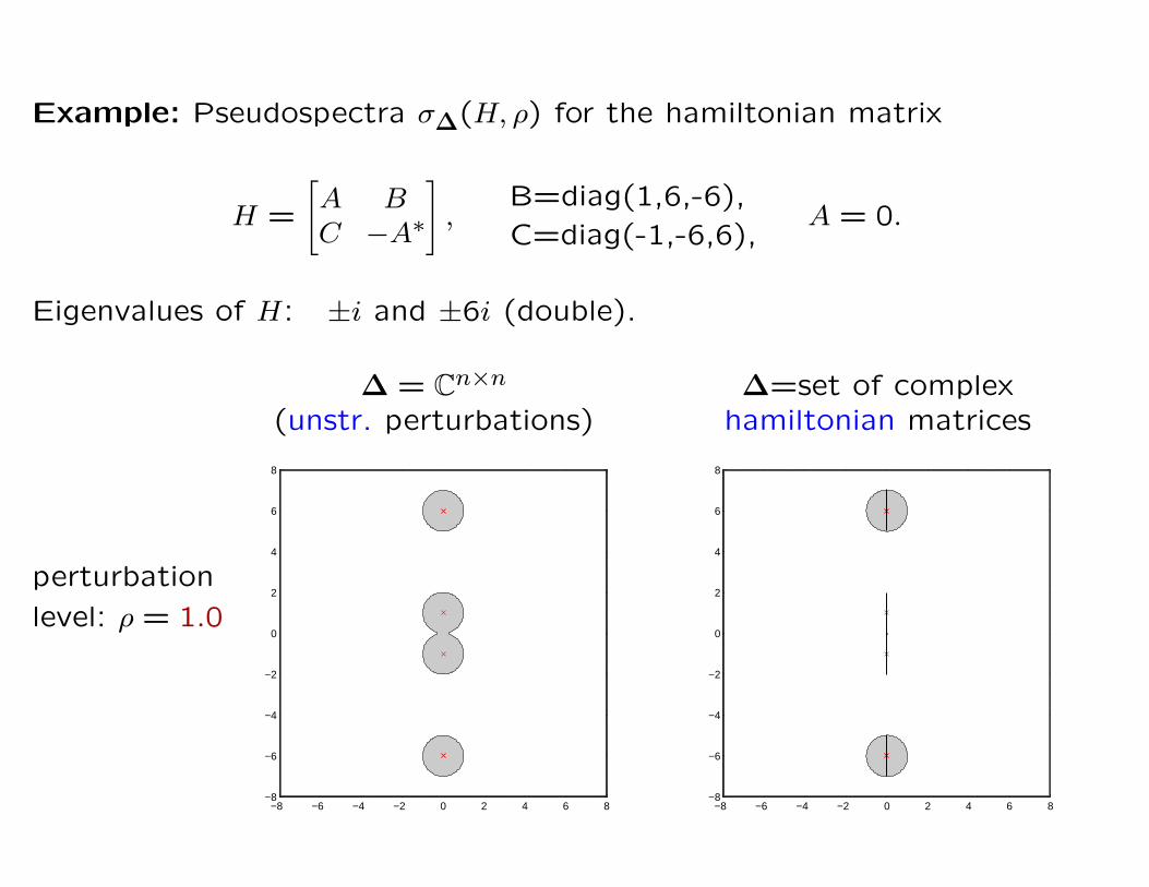
Example: Pseudospectra σ∆(H, ρ) for the hamiltonian matrix
H =
[A BC −A∗
],
B=diag(1,6,-6),
C=diag(-1,-6,6),A = 0.
Eigenvalues of H: ±i and ±6i (double).
∆ = Cn×n ∆=set of complex(unstr. perturbations) hamiltonian matrices
−8 −6 −4 −2 0 2 4 6 8−8
−6
−4
−2
0
2
4
6
8
−8 −6 −4 −2 0 2 4 6 8−8
−6
−4
−2
0
2
4
6
8
perturbation
level: ρ = 1.0
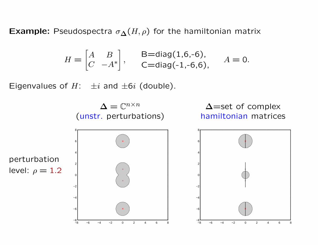
Example: Pseudospectra σ∆(H, ρ) for the hamiltonian matrix
H =
[A BC −A∗
],
B=diag(1,6,-6),
C=diag(-1,-6,6),A = 0.
Eigenvalues of H: ±i and ±6i (double).
∆ = Cn×n ∆=set of complex(unstr. perturbations) hamiltonian matrices
−8 −6 −4 −2 0 2 4 6 8−8
−6
−4
−2
0
2
4
6
8
−8 −6 −4 −2 0 2 4 6 8−8
−6
−4
−2
0
2
4
6
8
perturbation
level: ρ = 1.2
Example: Pseudospectra σ∆(H, ρ) for the hamiltonian matrix
H =
[A BC −A∗
],
B=diag(1,6,-6),
C=diag(-1,-6,6),A = 0.
Eigenvalues of H: ±i and ±6i (double).
∆ = Cn×n ∆=set of complex(unstr. perturbations) hamiltonian matrices
−8 −6 −4 −2 0 2 4 6 8−8
−6
−4
−2
0
2
4
6
8
−8 −6 −4 −2 0 2 4 6 8−8
−6
−4
−2
0
2
4
6
8
perturbation
level: ρ = 1.6

Example: Pseudospectra σ∆(H, ρ) for the hamiltonian matrix
H =
[A BC −A∗
],
B=diag(1,6,-6),
C=diag(-1,-6,6),A = 0.
Eigenvalues of H: ±i and ±6i (double).
∆ = Cn×n ∆=set of complex(unstr. perturbations) hamiltonian matrices
−8 −6 −4 −2 0 2 4 6 8−8
−6
−4
−2
0
2
4
6
8
−8 −6 −4 −2 0 2 4 6 8−8
−6
−4
−2
0
2
4
6
8
perturbation
level: ρ = 2.0

Example: Pseudospectra σ∆(H, ρ) for the hamiltonian matrix
H =
[A BC −A∗
],
B=diag(1,6,-6),
C=diag(-1,-6,6),A = 0.
Eigenvalues of H: ±i and ±6i (double).
∆ = Cn×n ∆=set of complex(unstr. perturbations) hamiltonian matrices
−8 −6 −4 −2 0 2 4 6 8−8
−6
−4
−2
0
2
4
6
8
−8 −6 −4 −2 0 2 4 6 8−8
−6
−4
−2
0
2
4
6
8
perturbation
level: ρ = 3.0
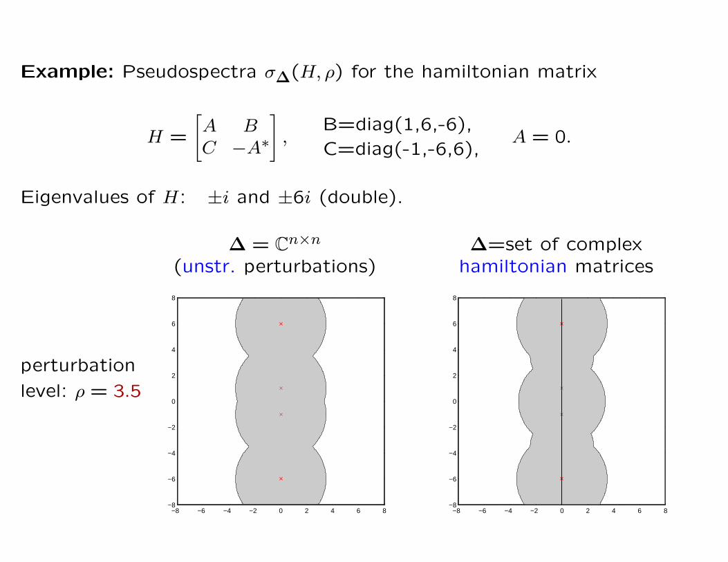
Example: Pseudospectra σ∆(H, ρ) for the hamiltonian matrix
H =
[A BC −A∗
],
B=diag(1,6,-6),
C=diag(-1,-6,6),A = 0.
Eigenvalues of H: ±i and ±6i (double).
∆ = Cn×n ∆=set of complex(unstr. perturbations) hamiltonian matrices
−8 −6 −4 −2 0 2 4 6 8−8
−6
−4
−2
0
2
4
6
8
−8 −6 −4 −2 0 2 4 6 8−8
−6
−4
−2
0
2
4
6
8
perturbation
level: ρ = 3.5
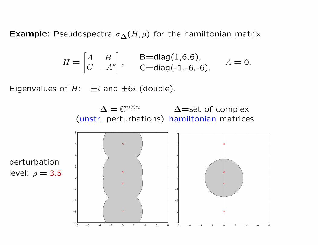
Example: Pseudospectra σ∆(H, ρ) for the hamiltonian matrix
H =
[A BC −A∗
],
B=diag(1,6,6),
C=diag(-1,-6,-6),A = 0.
Eigenvalues of H: ±i and ±6i (double).
∆ = Cn×n ∆=set of complex(unstr. perturbations) hamiltonian matrices
−8 −6 −4 −2 0 2 4 6 8−8
−6
−4
−2
0
2
4
6
8
perturbation
level: ρ = 3.5
−8 −6 −4 −2 0 2 4 6 8−8
−6
−4
−2
0
2
4
6
8
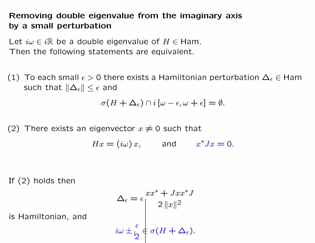
Removing double eigenvalue from the imaginary axis
by a small perturbation
Let iω ∈ iR be a double eigenvalue of H ∈ Ham.
Then the following statements are equivalent.
(1) To each small ε > 0 there exists a Hamiltonian perturbation ∆ε ∈ Ham
such that ‖∆ε‖ ≤ ε and
σ(H + ∆ε) ∩ i [ω − ε, ω + ε] = ∅.
(2) There exists an eigenvector x 6= 0 such that
Hx = (iω) x, and x∗Jx = 0.
If (2) holds then
∆ε = εxx∗ + Jxx∗J
2 ‖x‖2is Hamiltonian, and
iω ± ε
2∈ σ(H + ∆ε).
Small Perturbations:
Pseudospectra and eigenvalue condition numbers.
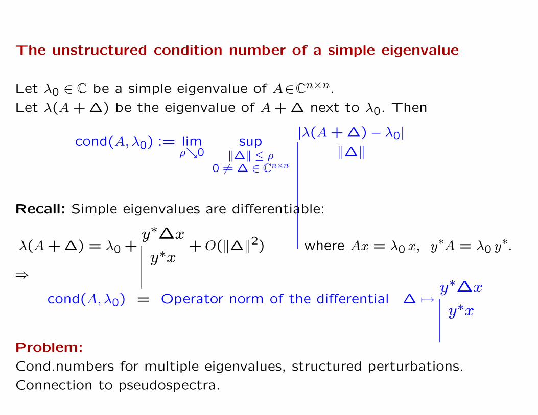
The unstructured condition number of a simple eigenvalue
Let λ0 ∈ C be a simple eigenvalue of A∈Cn×n.
Let λ(A + ∆) be the eigenvalue of A + ∆ next to λ0. Then
cond(A, λ0) := limρ↘0
sup‖∆‖ ≤ ρ
0 6= ∆ ∈ Cn×n
|λ(A + ∆) − λ0|‖∆‖
Recall: Simple eigenvalues are differentiable:
λ(A + ∆) = λ0 +y∗∆x
y∗x+ O(‖∆‖2) where Ax = λ0 x, y∗A = λ0 y∗.
⇒cond(A, λ0) = Operator norm of the differential ∆ 7→
y∗∆x
y∗x
Problem:
Cond.numbers for multiple eigenvalues, structured perturbations.
Connection to pseudospectra.
ρ = .10
−10 −8 −6 −4 −2 0 2 4 6 8 10
−10
−8
−6
−4
−2
0
2
4
6
8
10
ρ = .07
−10 −8 −6 −4 −2 0 2 4 6 8 10
−10
−8
−6
−4
−2
0
2
4
6
8
10
ρ = .02
−10 −8 −6 −4 −2 0 2 4 6 8 10
−10
−8
−6
−4
−2
0
2
4
6
8
10
ρ = .10
−10 −8 −6 −4 −2 0 2 4 6 8 10
−10
−8
−6
−4
−2
0
2
4
6
8
10
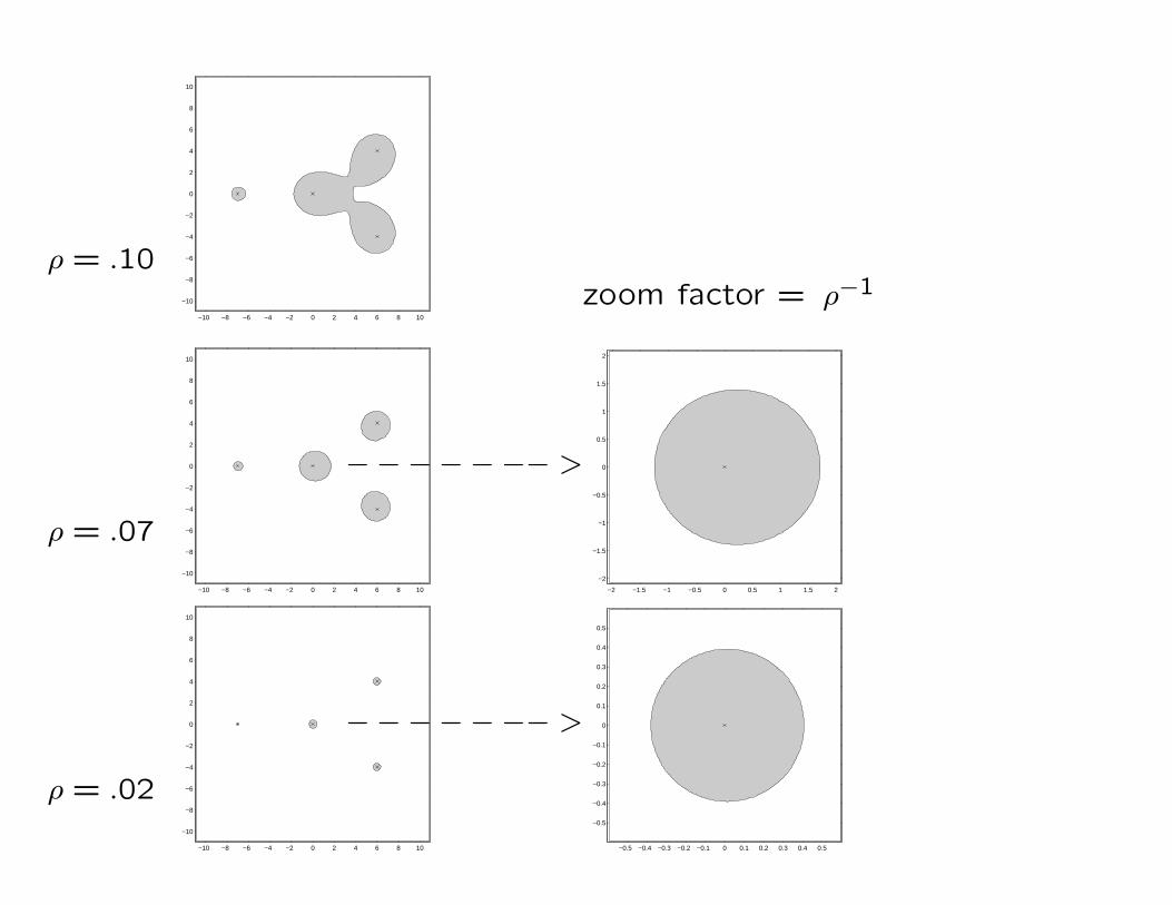
zoom factor = ρ−1
ρ = .07
−10 −8 −6 −4 −2 0 2 4 6 8 10
−10
−8
−6
−4
−2
0
2
4
6
8
10
−2 −1.5 −1 −0.5 0 0.5 1 1.5 2
−2
−1.5
−1
−0.5
0
0.5
1
1.5
2
−−−−−−− >
ρ = .02
−10 −8 −6 −4 −2 0 2 4 6 8 10
−10
−8
−6
−4
−2
0
2
4
6
8
10
−0.5 −0.4 −0.3 −0.2 −0.1 0 0.1 0.2 0.3 0.4 0.5
−0.5
−0.4
−0.3
−0.2
−0.1
0
0.1
0.2
0.3
0.4
0.5
−−−−−−− >
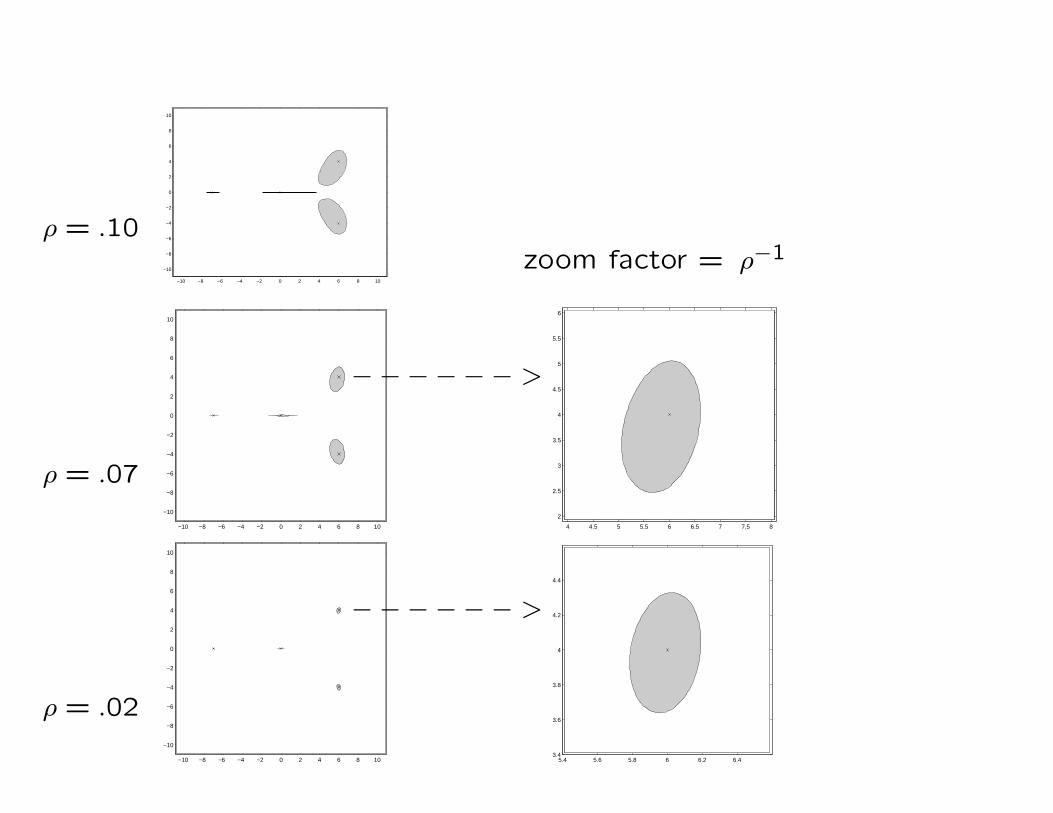
ρ = .10
−10 −8 −6 −4 −2 0 2 4 6 8 10
−10
−8
−6
−4
−2
0
2
4
6
8
10
zoom factor = ρ−1
ρ = .07
−10 −8 −6 −4 −2 0 2 4 6 8 10
−10
−8
−6
−4
−2
0
2
4
6
8
10
4 4.5 5 5.5 6 6.5 7 7.5 8
2
2.5
3
3.5
4
4.5
5
5.5
6
−−−−−− >
ρ = .02
−10 −8 −6 −4 −2 0 2 4 6 8 10
−10
−8
−6
−4
−2
0
2
4
6
8
10
5.4 5.6 5.8 6 6.2 6.43.4
3.6
3.8
4
4.2
4.4
−−−−−− >
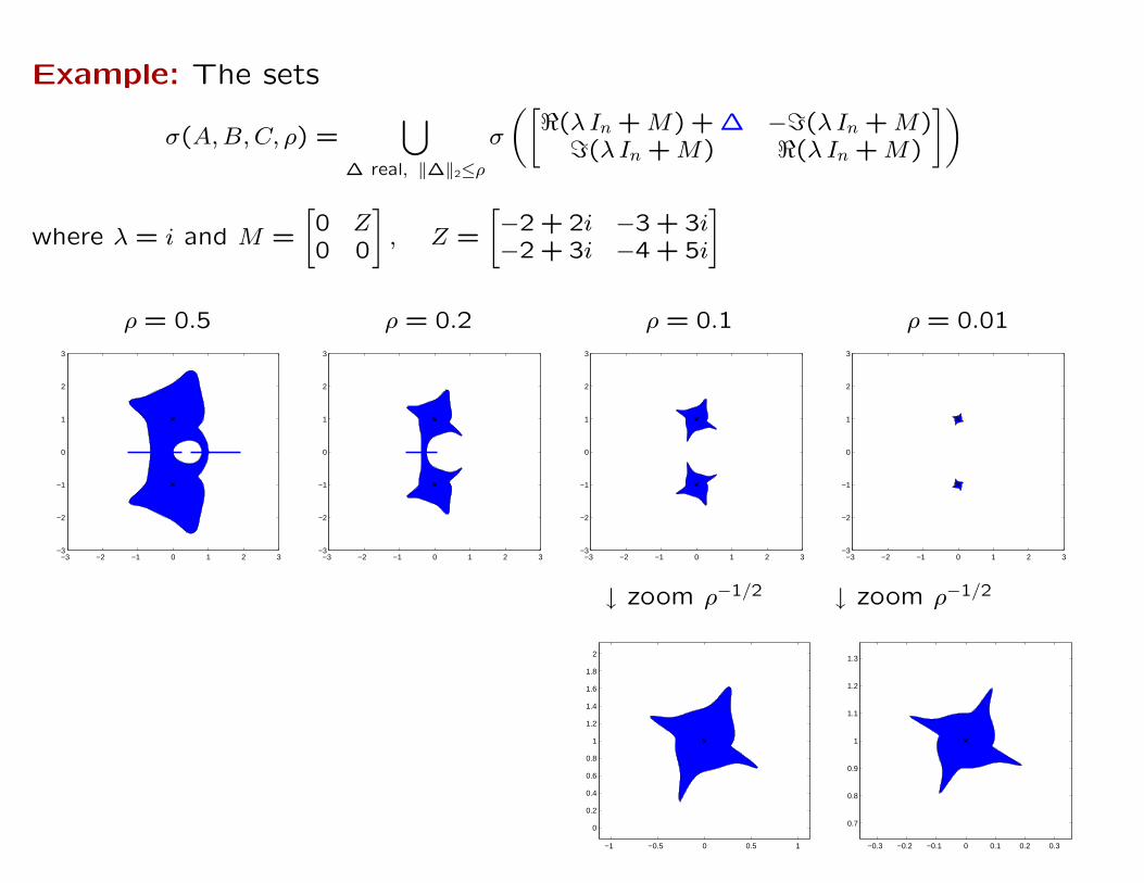
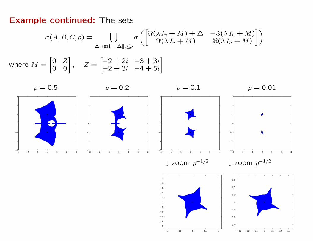
Example: The sets
σ(A, B, C, ρ) =⋃
∆ real, ‖∆‖2≤ρ
σ
([<(λ In + M) + ∆ −=(λ In + M)
=(λ In + M) <(λ In + M)
])
where λ = i and M =
[0 Z0 0
], Z =
[−2 + 2i −3 + 3i−2 + 3i −4 + 5i
]
ρ = 0.5 ρ = 0.2 ρ = 0.1 ρ = 0.01
−3 −2 −1 0 1 2 3−3
−2
−1
0
1
2
3
−3 −2 −1 0 1 2 3−3
−2
−1
0
1
2
3
−3 −2 −1 0 1 2 3−3
−2
−1
0
1
2
3
−3 −2 −1 0 1 2 3−3
−2
−1
0
1
2
3
↓ zoom ρ−1/2 ↓ zoom ρ−1/2
−1 −0.5 0 0.5 1
0
0.2
0.4
0.6
0.8
1
1.2
1.4
1.6
1.8
2
−0.3 −0.2 −0.1 0 0.1 0.2 0.3
0.7
0.8
0.9
1
1.1
1.2
1.3
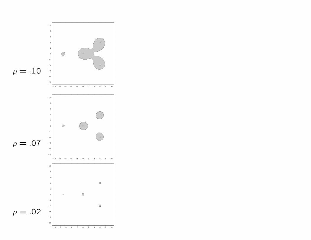
In the examples we have seen:
If properly scaled the connected components of
the spectral value sets σ∆(A, B, C, ρ) converge
to limit sets Lλ as ρ → 0.
Questions:
1. What is the right scaling?
2. How can the limit sets be computed?
To answer these questions one needs the
partial fraction decomposition of G(s) = C(sI − A)−1B
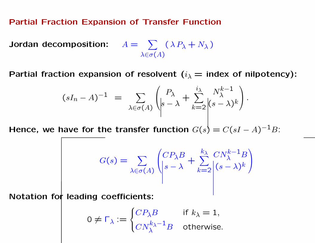
Partial Fraction Expansion of Transfer Function
Jordan decomposition: A =∑
λ∈σ(A)
(λ Pλ + Nλ )
Partial fraction expansion of resolvent (iλ = index of nilpotency):
(sIn − A)−1 =∑
λ∈σ(A)
Pλ
s − λ+
iλ∑
k=2
Nk−1λ
(s − λ)k
.
Hence, we have for the transfer function G(s) = C(sI − A)−1B:
G(s) =∑
λ∈σ(A)
CPλB
s − λ+
kλ∑
k=2
CNk−1λ B
(s − λ)k
Notation for leading coefficients:
0 6= Γλ :=
CPλB if kλ = 1,
CNkλ−1λ B otherwise.
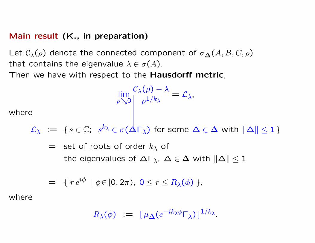
Main result (K., in preparation)
Let Cλ(ρ) denote the connected component of σ∆(A, B, C, ρ)
that contains the eigenvalue λ ∈ σ(A).
Then we have with respect to the Hausdorff metric,
limρ↘0
Cλ(ρ) − λ
ρ1/kλ= Lλ,
where
Lλ := { s ∈ C; skλ ∈ σ(∆Γλ) for some ∆ ∈ ∆ with ‖∆‖ ≤ 1 }
= set of roots of order kλ of
the eigenvalues of ∆Γλ, ∆ ∈ ∆ with ‖∆‖ ≤ 1
= { r eiφ | φ∈ [0,2π), 0 ≤ r ≤ Rλ(φ) },where
Rλ(φ) := [µ∆(e−ikλφΓλ) ]1/kλ.

Radius of limit set equals the condition number
−5 0 5
−5
−4
−3
−2
−1
0
1
2
3
4
5
Limit Set
Condition Number
For small ρ,
Cλ(ρ) ≈ λ + ρ1/kλ Lλ
⇒
condition number := max{ |s|; s ∈ Lλ } = maxφ∈[0,2π]
[µ∆(e−ikλφΓλ) ]1/kλ
For an approach to condition numbers via Puisseux-series see paper by
Kressner, Moro, Pelaez (2006).
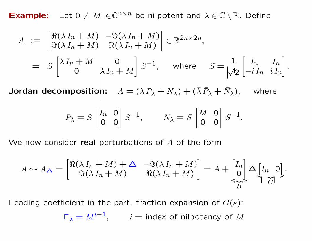
Example: Let 0 6= M ∈Cn×n be nilpotent and λ ∈ C \ R. Define
A :=
[<(λ In + M) −=(λ In + M)=(λ In + M) <(λ In + M)
]∈ R
2n×2n,
= S
[λ In + M 0
0 λ In + M
]S−1, where S =
1√2
[In In
−i In i In
].
Jordan decomposition: A = (λ Pλ + Nλ) + (λ Pλ + Nλ), where
Pλ = S
[In 00 0
]S−1, Nλ = S
[M 00 0
]S−1.
We now consider real perturbations of A of the form
A ; A∆ =
[<(λ In + M) + ∆ −=(λ In + M)
=(λ In + M) <(λ In + M)
]= A +
[In
0
]
︸ ︷︷ ︸B
∆[In 0
]
︸ ︷︷ ︸C
.
Leading coefficient in the part. fraction expansion of G(s):
Γλ = M i−1, i = index of nilpotency of M
Example continued: The sets
σ(A, B, C, ρ) =⋃
∆ real, ‖∆‖2≤ρ
σ
([<(λ In + M) + ∆ −=(λ In + M)
=(λ In + M) <(λ In + M)
])
where M =
[0 Z0 0
], Z =
[−2 + 2i −3 + 3i−2 + 3i −4 + 5i
]
ρ = 0.5 ρ = 0.2 ρ = 0.1 ρ = 0.01
−3 −2 −1 0 1 2 3−3
−2
−1
0
1
2
3
−3 −2 −1 0 1 2 3−3
−2
−1
0
1
2
3
−3 −2 −1 0 1 2 3−3
−2
−1
0
1
2
3
−3 −2 −1 0 1 2 3−3
−2
−1
0
1
2
3
↓ zoom ρ−1/2 ↓ zoom ρ−1/2
−1 −0.5 0 0.5 1
0
0.2
0.4
0.6
0.8
1
1.2
1.4
1.6
1.8
2
−0.3 −0.2 −0.1 0 0.1 0.2 0.3
0.7
0.8
0.9
1
1.1
1.2
1.3
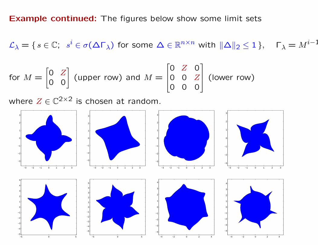
Example continued: The figures below show some limit sets
Lλ = { s ∈ C; si ∈ σ(∆Γλ) for some ∆ ∈ Rn×n with ‖∆‖2 ≤ 1 }, Γλ = M i−1
for M =
[0 Z0 0
](upper row) and M =
0 Z 00 0 Z0 0 0
(lower row)
where Z ∈ C2×2 is chosen at random.
−3 −2 −1 0 1 2 3
−3
−2
−1
0
1
2
3
−3 −2 −1 0 1 2 3
−3
−2
−1
0
1
2
3
−3 −2 −1 0 1 2 3
−3
−2
−1
0
1
2
3
−3 −2 −1 0 1 2 3
−3
−2
−1
0
1
2
3
−5 0 5−5
−4
−3
−2
−1
0
1
2
3
4
5
−5 0 5
−5
−4
−3
−2
−1
0
1
2
3
4
5
−4 −2 0 2 4
−4
−3
−2
−1
0
1
2
3
4
−4 −2 0 2 4
−4
−3
−2
−1
0
1
2
3
4
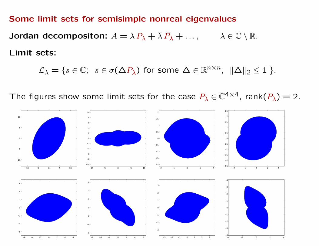
Some limit sets for semisimple nonreal eigenvalues
Jordan decompositon: A = λ Pλ + λ Pλ + . . . , λ ∈ C \ R.
Limit sets:
Lλ = {s ∈ C; s ∈ σ(∆Pλ) for some ∆ ∈ Rn×n, ‖∆‖2 ≤ 1 }.
The figures show some limit sets for the case Pλ ∈ C4×4, rank(Pλ) = 2.
−10 −5 0 5 10
−10
−5
0
5
10
−10 −5 0 5 10
−10
−8
−6
−4
−2
0
2
4
6
8
10
−2 −1 0 1 2
−2
−1.5
−1
−0.5
0
0.5
1
1.5
2
−2 −1 0 1 2−2.5
−2
−1.5
−1
−0.5
0
0.5
1
1.5
2
2.5
−6 −4 −2 0 2 4 6
−6
−4
−2
0
2
4
6
−6 −4 −2 0 2 4 6
−6
−4
−2
0
2
4
6
−3 −2 −1 0 1 2 3
−3
−2
−1
0
1
2
3
−4 −2 0 2 4−4
−3
−2
−1
0
1
2
3
4
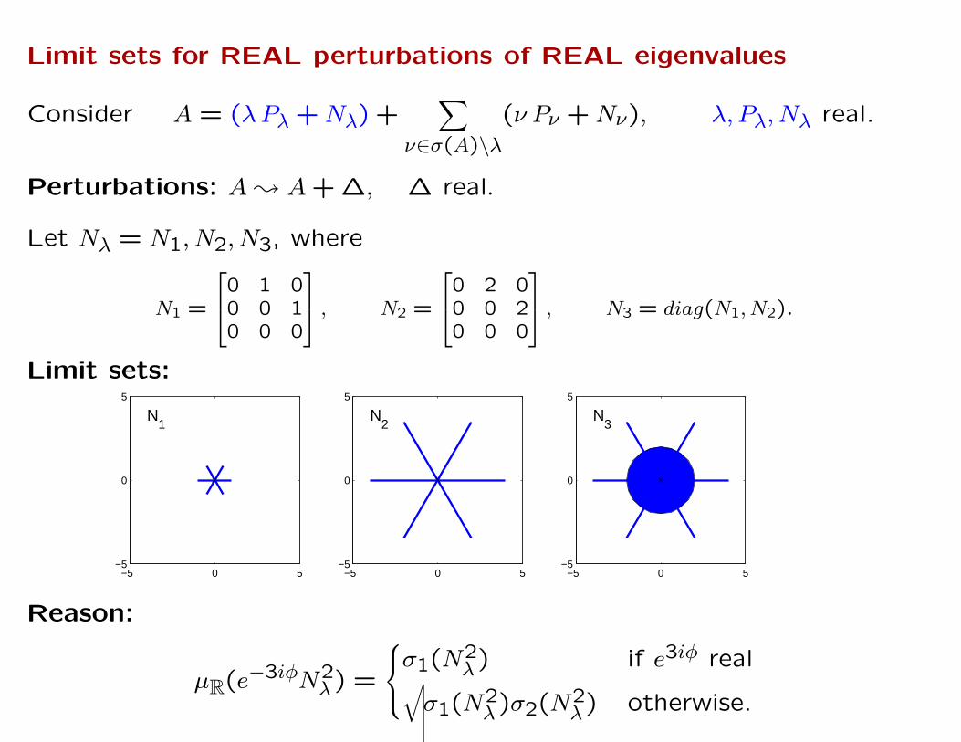
Limit sets for REAL perturbations of REAL eigenvalues
Consider A = (λ Pλ + Nλ) +∑
ν∈σ(A)\λ(ν Pν + Nν), λ, Pλ, Nλ real.
Perturbations: A ; A + ∆, ∆ real.
Let Nλ = N1, N2, N3, where
N1 =
0 1 00 0 10 0 0
, N2 =
0 2 00 0 20 0 0
, N3 = diag(N1, N2).
Limit sets:
−5 0 5−5
0
5
N1
−5 0 5−5
0
5
N2
−5 0 5−5
0
5
N3
Reason:
µR(e−3iφN2λ) =
σ1(N2λ) if e3iφ real
√σ1(N
2λ)σ2(N
2λ) otherwise.
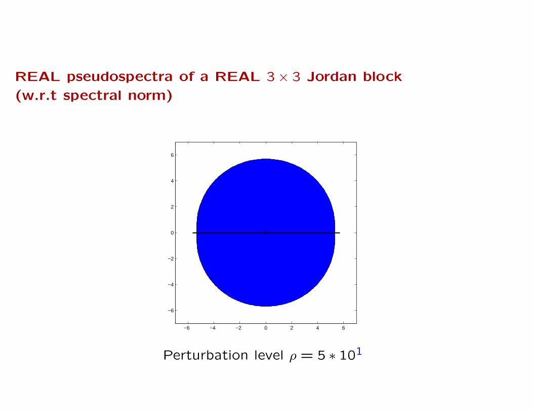
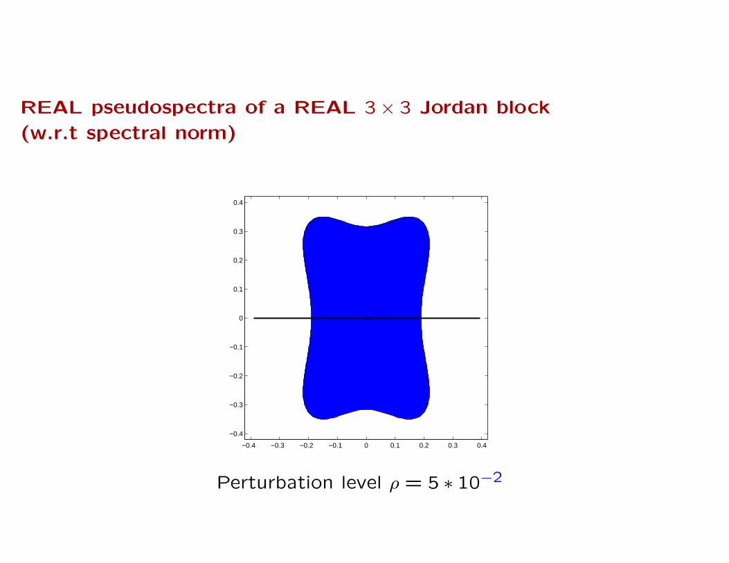
REAL pseudospectra of a REAL 3 × 3 Jordan block
(w.r.t spectral norm)
−6 −4 −2 0 2 4 6
−6
−4
−2
0
2
4
6
Perturbation level ρ = 5 ∗ 101
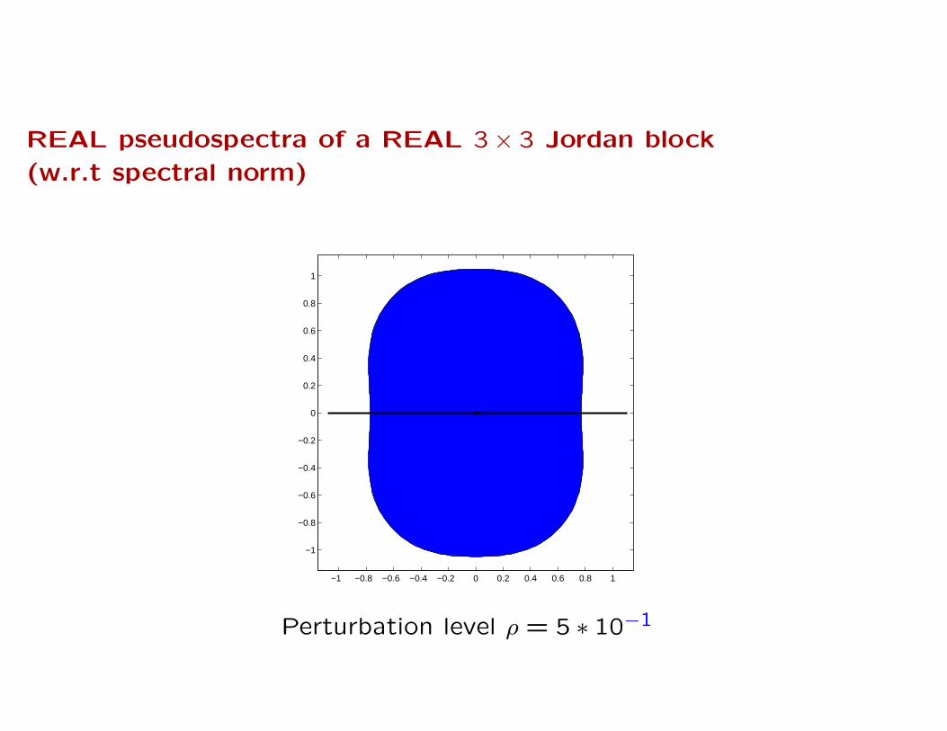
REAL pseudospectra of a REAL 3 × 3 Jordan block
(w.r.t spectral norm)
−1 −0.8 −0.6 −0.4 −0.2 0 0.2 0.4 0.6 0.8 1
−1
−0.8
−0.6
−0.4
−0.2
0
0.2
0.4
0.6
0.8
1
Perturbation level ρ = 5 ∗ 10−1
REAL pseudospectra of a REAL 3 × 3 Jordan block
(w.r.t spectral norm)
−0.4 −0.3 −0.2 −0.1 0 0.1 0.2 0.3 0.4
−0.4
−0.3
−0.2
−0.1
0
0.1
0.2
0.3
0.4
Perturbation level ρ = 5 ∗ 10−2
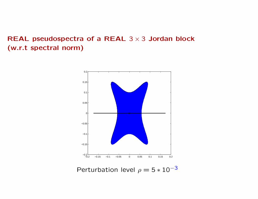
REAL pseudospectra of a REAL 3 × 3 Jordan block
(w.r.t spectral norm)
−0.2 −0.15 −0.1 −0.05 0 0.05 0.1 0.15 0.2−0.2
−0.15
−0.1
−0.05
0
0.05
0.1
0.15
0.2
Perturbation level ρ = 5 ∗ 10−3
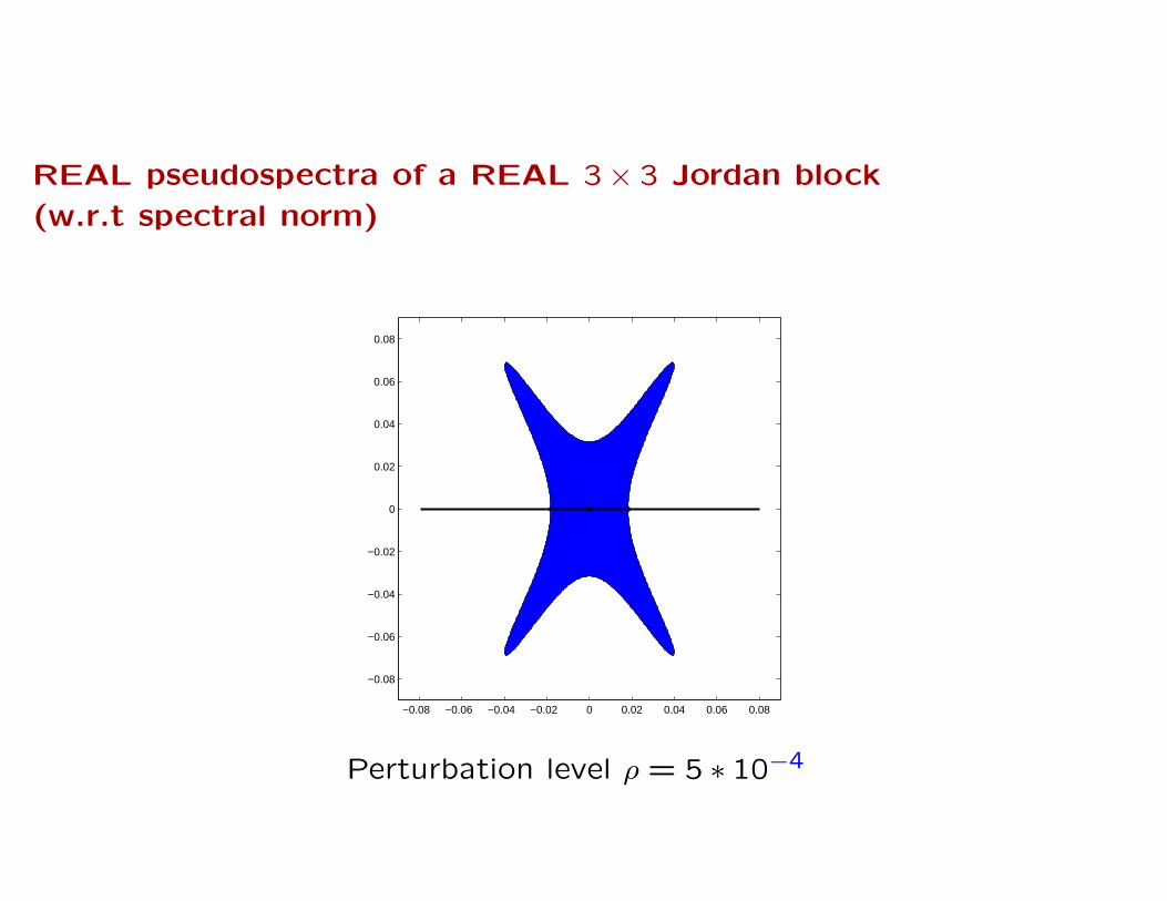
REAL pseudospectra of a REAL 3 × 3 Jordan block
(w.r.t spectral norm)
−0.08 −0.06 −0.04 −0.02 0 0.02 0.04 0.06 0.08
−0.08
−0.06
−0.04
−0.02
0
0.02
0.04
0.06
0.08
Perturbation level ρ = 5 ∗ 10−4
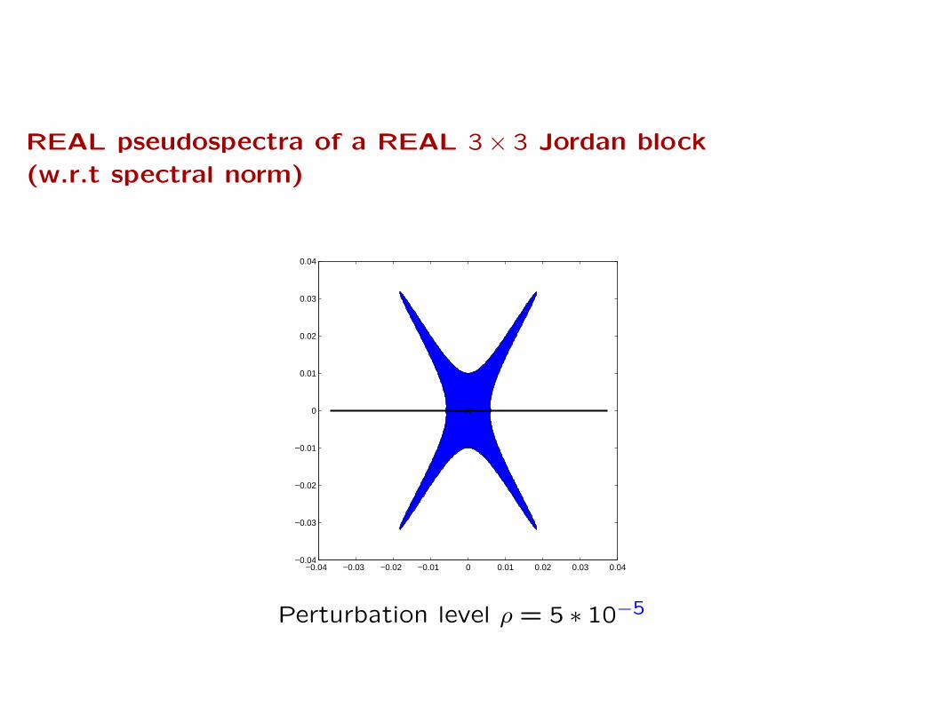
REAL pseudospectra of a REAL 3 × 3 Jordan block
(w.r.t spectral norm)
−0.04 −0.03 −0.02 −0.01 0 0.01 0.02 0.03 0.04−0.04
−0.03
−0.02
−0.01
0
0.01
0.02
0.03
0.04
Perturbation level ρ = 5 ∗ 10−5
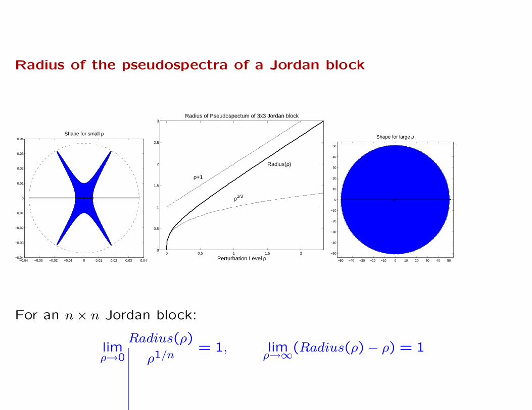
Radius of the pseudospectra of a Jordan block
−0.04 −0.03 −0.02 −0.01 0 0.01 0.02 0.03 0.04−0.04
−0.03
−0.02
−0.01
0
0.01
0.02
0.03
0.04Shape for small ρ
0 0.5 1 1.5 20
0.5
1
1.5
2
2.5
3
ρ+1
ρ1/3
Radius(ρ)
Perturbation Level ρ
Radius of Pseudospectum of 3x3 Jordan block
−50 −40 −30 −20 −10 0 10 20 30 40 50
−50
−40
−30
−20
−10
0
10
20
30
40
50
Shape for large ρ
For an n × n Jordan block:
limρ→0
Radius(ρ)
ρ1/n= 1, lim
ρ→∞(Radius(ρ) − ρ) = 1
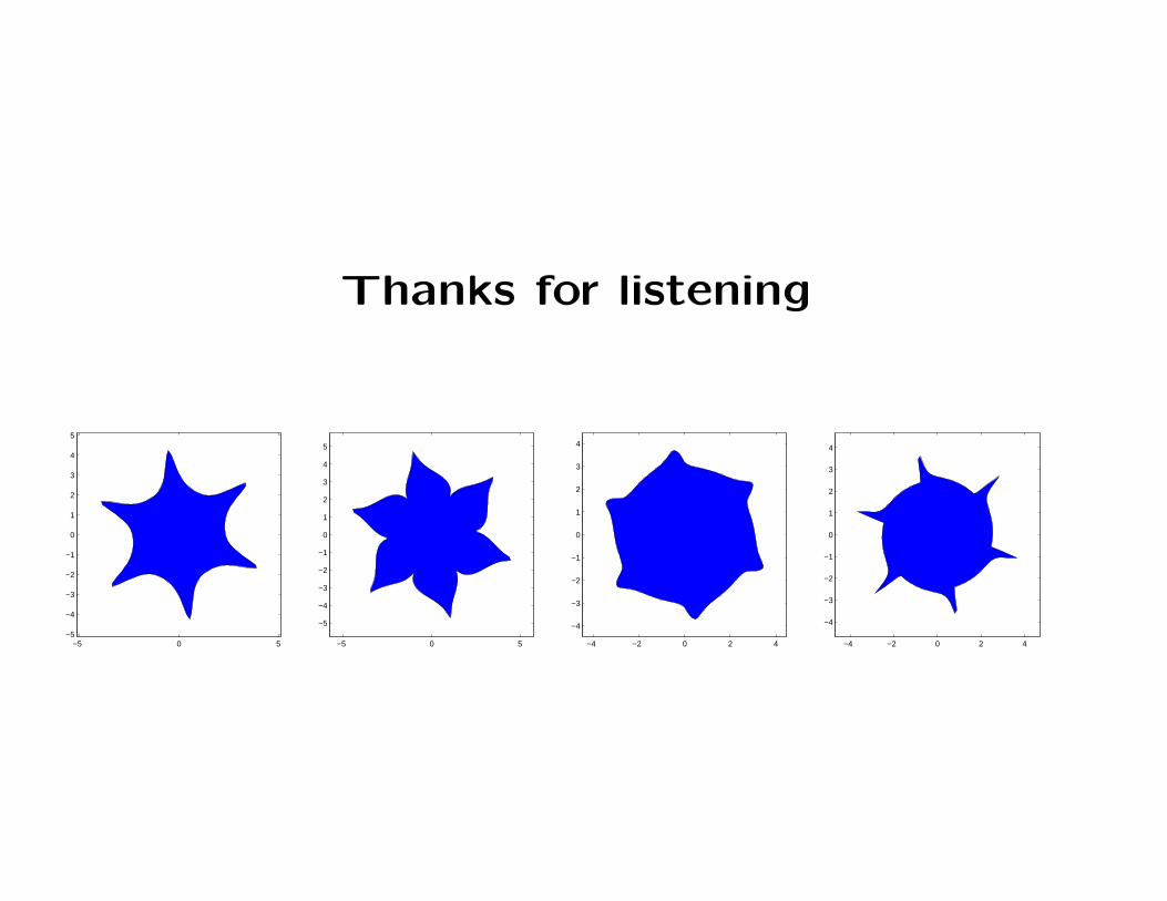
Thanks for listening
−5 0 5−5
−4
−3
−2
−1
0
1
2
3
4
5
−5 0 5
−5
−4
−3
−2
−1
0
1
2
3
4
5
−4 −2 0 2 4
−4
−3
−2
−1
0
1
2
3
4
−4 −2 0 2 4
−4
−3
−2
−1
0
1
2
3
4