PS6-DCT-Soln-correction

Unknown Author

March 18, 2014

Part I

DCT: Discrete Cosine TransformDCT is a linear map A ∈ RN×N such that the N real numbers x0, . . . , xN−1 are transformed into the N real numbersX0, . . . , XN−1 according to the formula

Xk = x0 + 2

N−1∑i=1

xi cos

(π

N(k +

1

2)i

). (1)

1 Question 1:

Consider the case where N = 2. Write Python function using (1) to compute X0, X1 given x0, x1. Specifically yourfunction should take in x0, x1 as arguments and return X0, X1.

In [1]: import numpy as np""" Your code goes here """def f(x0,x1):

N=2X0=x0+2*x1*np.cos(np.pi/N*(1+1/2)*0)X1=x0+2*x1*np.cos(np.pi/N*(1+1/2)*1)return X0,X1

def vald(i,k):N=8return 2*np.cos((np.pi/N) * i * (k + 0.5) ) #x[n]*cos(pi*(k+0.5)*n/N)

Verify that your function works by computing X0, X1 given x0 = 2, x1 = 4.

In [2]: np.set_printoptions(precision=3)""" Check your function here """y=f(2.0,4.0)print "%.2f "*len(y) % y

10.00 2.00

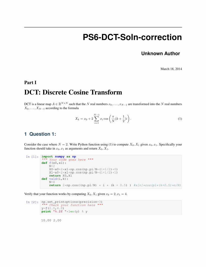
2 Question 2:

JPEG compression uses the DCT withN = 8. Create a matrix calledD that is the matrix representation of the discretecosine transform, i.e. when you multiply D by the vector x0

...xN−1

you should get the vector X0

...XN−1

In [3]: """ your code goes here"""

N = 8D = np.zeros((N, N))for i in range(N):

D[0,i] = 1for i in xrange(1,N):

for k in xrange(N):D[i,k] = 2*np.cos((np.pi/N) * i * (k + 0.5) )

D=D.Tprint D

[[ 1. 1.962 1.848 1.663 1.414 1.111 0.765 0.39 ][ 1. 1.663 0.765 -0.39 -1.414 -1.962 -1.848 -1.111][ 1. 1.111 -0.765 -1.962 -1.414 0.39 1.848 1.663][ 1. 0.39 -1.848 -1.111 1.414 1.663 -0.765 -1.962][ 1. -0.39 -1.848 1.111 1.414 -1.663 -0.765 1.962][ 1. -1.111 -0.765 1.962 -1.414 -0.39 1.848 -1.663][ 1. -1.663 0.765 0.39 -1.414 1.962 -1.848 1.111][ 1. -1.962 1.848 -1.663 1.414 -1.111 0.765 -0.39 ]]

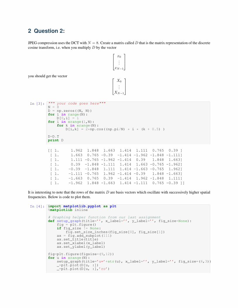
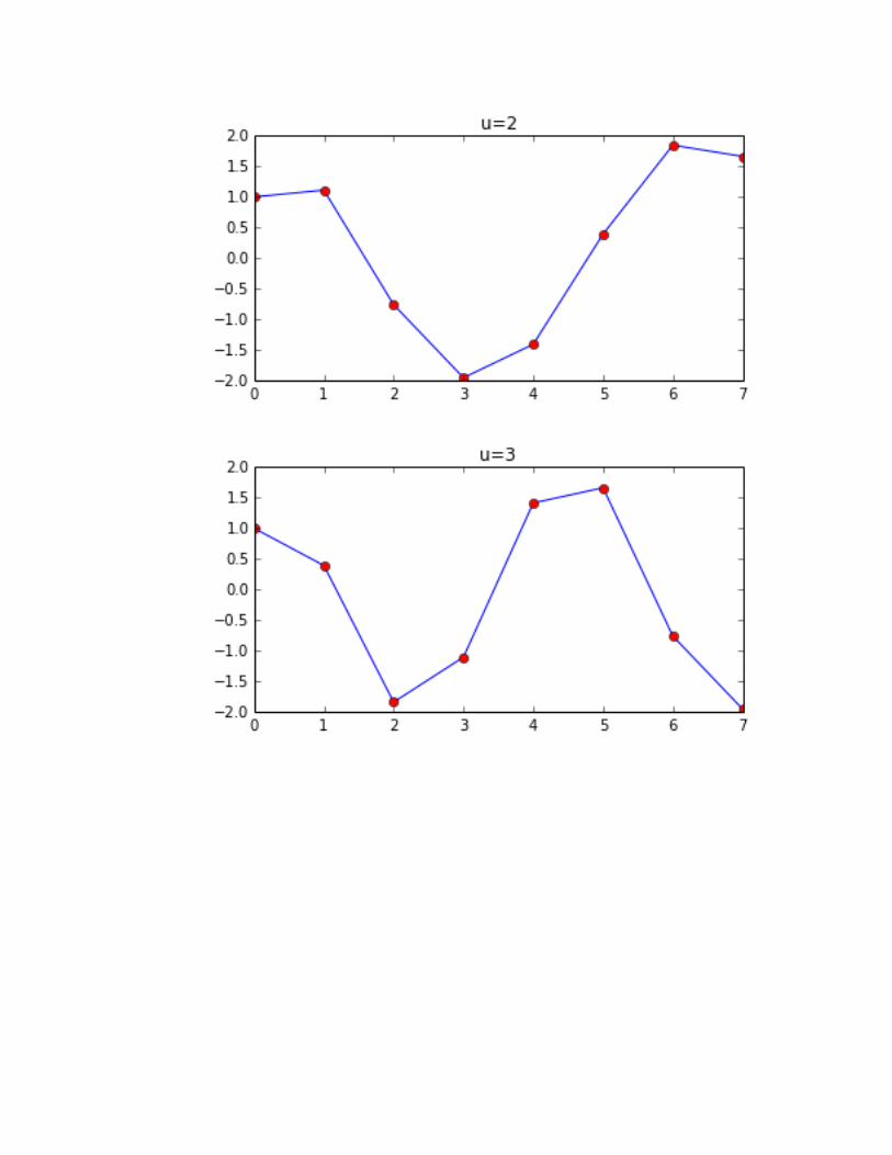
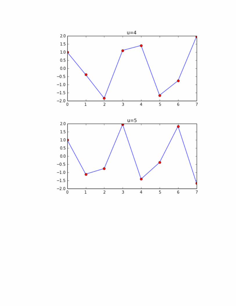
It is interesting to note that the rows of the matrix D are basis vectors which oscillate with successively higher spatialfrequencies. Below is code to plot them.

In [4]: import matplotlib.pyplot as plt%matplotlib inline

# Graphing helper function from our last assignmentdef setup_graph(title=’’, x_label=’’, y_label=’’, fig_size=None):

fig = plt.figure()if fig_size != None:

fig.set_size_inches(fig_size[0], fig_size[1])ax = fig.add_subplot(111)ax.set_title(title)ax.set_xlabel(x_label)ax.set_ylabel(y_label)

fig=plt.figure(figsize=(9,12))for u in xrange(N):

setup_graph(title=’u=’+str(u), x_label=’’, y_label=’’, fig_size=(6,3))_=plt.plot(D[u, :])_=plt.plot(D[u, :],’ro’)

<matplotlib.figure.Figure at 0x10f068490>

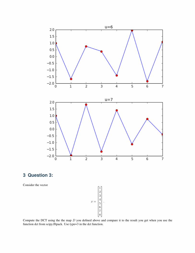
3 Question 3:

Consider the vector

x =

12345678

.

Compute the DCT using the the map D you defined above and compare it to the result you get when you use thefunction dct from scipy.fftpack. Use type=3 in the dct function.

In [6]: from scipy.fftpack import dct, idctx=np.array([[1.0, 2, 3, 4, 5, 6, 7, 8]])""" Your Code Goes Here"""print np.dot(D,x.T)print (dct(x,type=3)).T

[[ 39.335][-35.603][ 14.588][-12.209][ 6.549][ -5.453][ 2.184][ -1.391]]

[[ 39.335][-35.603][ 14.588][-12.209][ 6.549][ -5.453][ 2.184][ -1.391]]

4 Question 4:

Now, we will take the image we have provided you with and apply the 2D DCT to it.

In [7]: import matplotlib.image as mpimgimg = mpimg.imread(’montyPython.png’)p=plt.imshow(img, origin=’upper’)

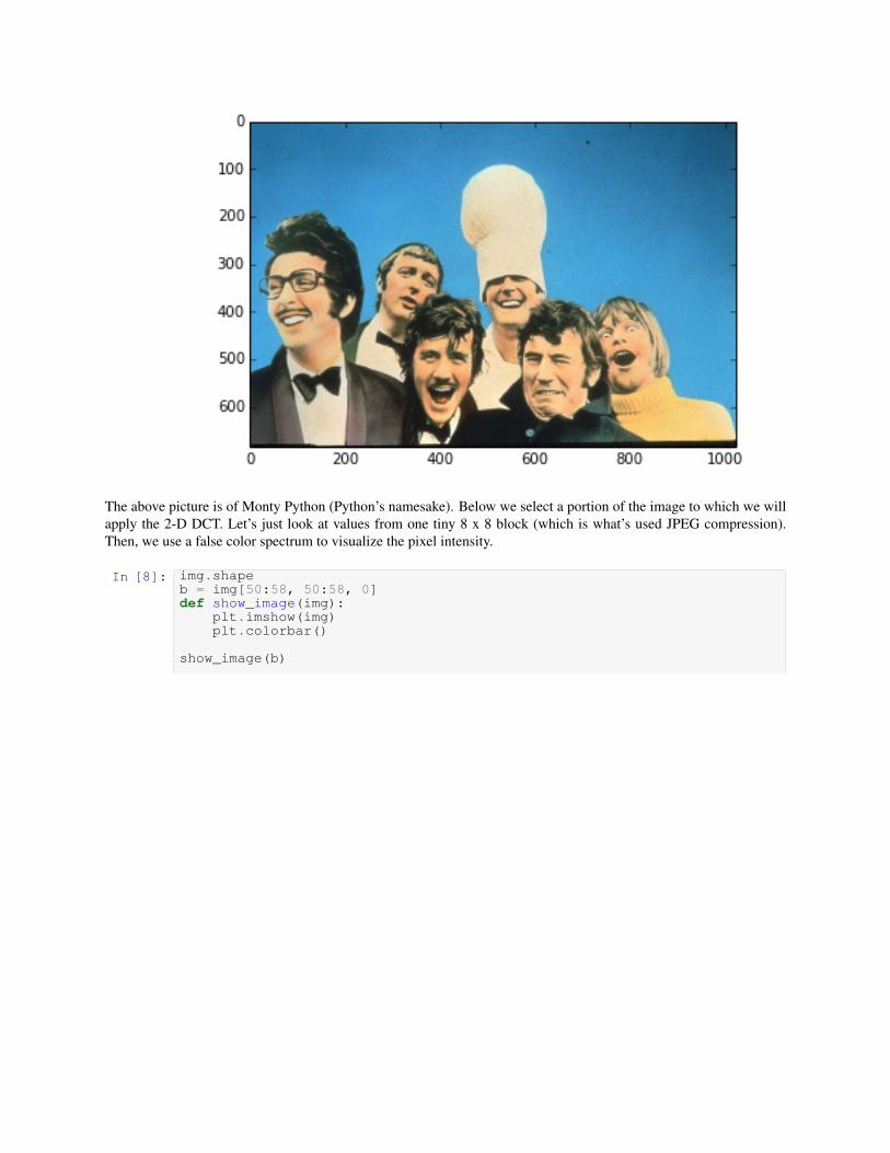
The above picture is of Monty Python (Python’s namesake). Below we select a portion of the image to which we willapply the 2-D DCT. Let’s just look at values from one tiny 8 x 8 block (which is what’s used JPEG compression).Then, we use a false color spectrum to visualize the pixel intensity.

In [8]: img.shapeb = img[50:58, 50:58, 0]def show_image(img):

plt.imshow(img)plt.colorbar()

show_image(b)

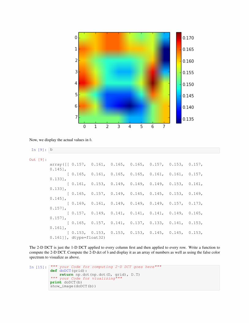
Now, we display the actual values in b.

In [9]: b

Out [9]:array([[ 0.157, 0.161, 0.165, 0.165, 0.157, 0.153, 0.157,0.145],

[ 0.165, 0.161, 0.165, 0.165, 0.161, 0.161, 0.157,0.133],

[ 0.161, 0.153, 0.149, 0.149, 0.149, 0.153, 0.161,0.133],

[ 0.165, 0.157, 0.149, 0.145, 0.145, 0.153, 0.169,0.145],

[ 0.169, 0.161, 0.149, 0.149, 0.149, 0.157, 0.173,0.157],

[ 0.157, 0.149, 0.141, 0.141, 0.141, 0.149, 0.165,0.157],

[ 0.165, 0.157, 0.141, 0.137, 0.133, 0.141, 0.153,0.161],

[ 0.153, 0.153, 0.153, 0.153, 0.145, 0.145, 0.153,0.161]], dtype=float32)

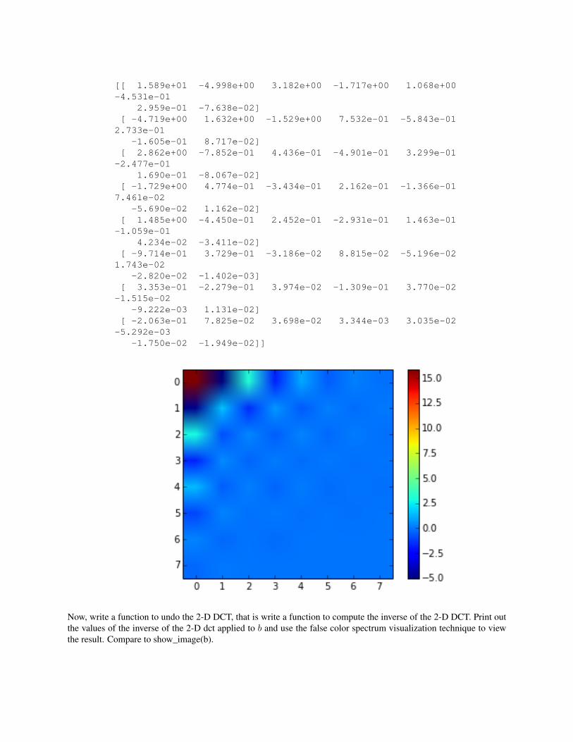
The 2-D DCT is just the 1-D DCT applied to every column first and then applied to every row. Write a function tocompute the 2-D DCT. Compute the 2-D dct of b and display it as an array of numbers as well as using the false colorspectrum to visualize as above.

In [15]: """ your Code for computing 2-D DCT goes here"""def doDCT(grid):

return np.dot(np.dot(D, grid), D.T)""" your Code for viualizing"""print doDCT(b)show_image(doDCT(b))

[[ 1.589e+01 -4.998e+00 3.182e+00 -1.717e+00 1.068e+00-4.531e-01

2.959e-01 -7.638e-02][ -4.719e+00 1.632e+00 -1.529e+00 7.532e-01 -5.843e-01

2.733e-01-1.605e-01 8.717e-02]

[ 2.862e+00 -7.852e-01 4.436e-01 -4.901e-01 3.299e-01-2.477e-01

1.690e-01 -8.067e-02][ -1.729e+00 4.774e-01 -3.434e-01 2.162e-01 -1.366e-01

7.461e-02-5.690e-02 1.162e-02]

[ 1.485e+00 -4.450e-01 2.452e-01 -2.931e-01 1.463e-01-1.059e-01

4.234e-02 -3.411e-02][ -9.714e-01 3.729e-01 -3.186e-02 8.815e-02 -5.196e-02

1.743e-02-2.820e-02 -1.402e-03]

[ 3.353e-01 -2.279e-01 3.974e-02 -1.309e-01 3.770e-02-1.515e-02

-9.222e-03 1.131e-02][ -2.063e-01 7.825e-02 3.698e-02 3.344e-03 3.035e-02

-5.292e-03-1.750e-02 -1.949e-02]]

Now, write a function to undo the 2-D DCT, that is write a function to compute the inverse of the 2-D DCT. Print outthe values of the inverse of the 2-D dct applied to b and use the false color spectrum visualization technique to viewthe result. Compare to show_image(b).

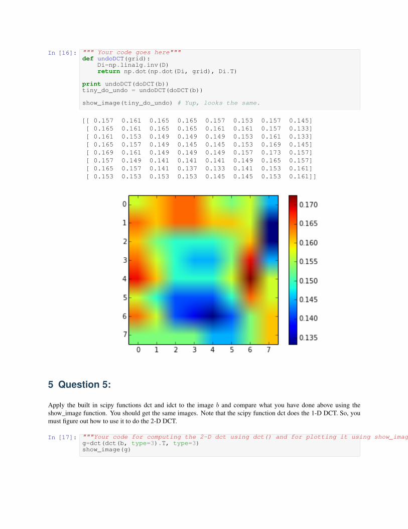
In [16]: """ Your code goes here"""def undoDCT(grid):

Di=np.linalg.inv(D)return np.dot(np.dot(Di, grid), Di.T)

print undoDCT(doDCT(b))tiny_do_undo = undoDCT(doDCT(b))

show_image(tiny_do_undo) # Yup, looks the same.

[[ 0.157 0.161 0.165 0.165 0.157 0.153 0.157 0.145][ 0.165 0.161 0.165 0.165 0.161 0.161 0.157 0.133][ 0.161 0.153 0.149 0.149 0.149 0.153 0.161 0.133][ 0.165 0.157 0.149 0.145 0.145 0.153 0.169 0.145][ 0.169 0.161 0.149 0.149 0.149 0.157 0.173 0.157][ 0.157 0.149 0.141 0.141 0.141 0.149 0.165 0.157][ 0.165 0.157 0.141 0.137 0.133 0.141 0.153 0.161][ 0.153 0.153 0.153 0.153 0.145 0.145 0.153 0.161]]

5 Question 5:

Apply the built in scipy functions dct and idct to the image b and compare what you have done above using theshow_image function. You should get the same images. Note that the scipy function dct does the 1-D DCT. So, youmust figure out how to use it to do the 2-D DCT.

In [17]: """Your code for computing the 2-D dct using dct() and for plotting it using show_image"""g=dct(dct(b, type=3).T, type=3)show_image(g)

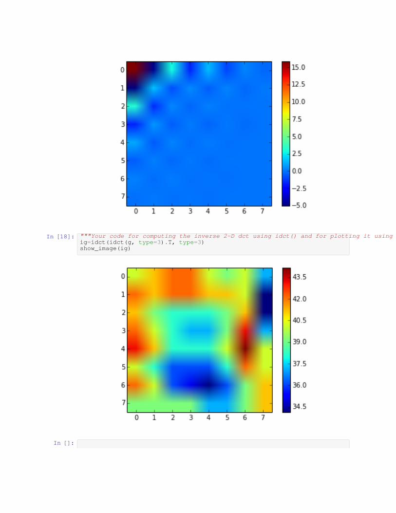
In [18]: """Your code for computing the inverse 2-D dct using idct() and for plotting it using show_image"""ig=idct(idct(g, type=3).T, type=3)show_image(ig)

In []: