Provable Bounds for Learning Some Deep Representations
54
Provable Bounds for Learning Some Deep Representations Sanjeev Arora * Aditya Bhaskara † Rong Ge ‡ Tengyu Ma § October 24, 2013 Abstract We give algorithms with provable guarantees that learn a class of deep nets in the generative model view popularized by Hinton and others. Our generative model is an n node multilayer neural net that has degree at most n γ for some γ< 1 and each edge has a random edge weight in [-1, 1]. Our algorithm learns almost all networks in this class with polynomial running time. The sample complexity is quadratic or cubic depending upon the details of the model. The algorithm uses layerwise learning. It is based upon a novel idea of observing correlations among features and using these to infer the underlying edge structure via a global graph recovery procedure. The analysis of the algorithm reveals interesting structure of neural networks with random edge weights. 1 1 Introduction Can we provide theoretical explanation for the practical success of deep nets? Like many other ML tasks, learning deep neural nets is NP-hard, and in fact seems “badly * Princeton University, Computer Science Department and Center for Computational Intractabil- ity. Email: [email protected]. This work is supported by the NSF grants CCF-0832797, CCF-1117309, CCF-1302518, DMS-1317308, and Simons Investigator Grant. † Google Research NYC. Email: [email protected]. The work was done while the author was a Postdoc at EPFL, Switzerland. ‡ Microsoft Research, New England. Email: [email protected]. Part of this work was done while the author was a graduate student at Princeton University and was supported in part by NSF grants CCF-0832797, CCF-1117309, CCF-1302518, DMS-1317308, and Simons Investigator Grant. § Princeton University, Computer Science Department and Center for Computational Intractabil- ity. Email: [email protected]. This work is supported by the NSF grants CCF-0832797, CCF-1117309, CCF-1302518, DMS-1317308, and Simons Investigator Grant. 1 The first 18 pages of this document serve as an extended abstract of the paper, and a long technical appendix follows. 1 arXiv:1310.6343v1 [cs.LG] 23 Oct 2013
Transcript of Provable Bounds for Learning Some Deep Representations
Provable Bounds for Learning Some DeepRepresentations
Sanjeev Arora∗ Aditya Bhaskara † Rong Ge‡ Tengyu Ma§
October 24, 2013
Abstract
We give algorithms with provable guarantees that learn a class of deep netsin the generative model view popularized by Hinton and others. Our generativemodel is an n node multilayer neural net that has degree at most nγ for someγ < 1 and each edge has a random edge weight in [−1, 1]. Our algorithm learnsalmost all networks in this class with polynomial running time. The samplecomplexity is quadratic or cubic depending upon the details of the model.
The algorithm uses layerwise learning. It is based upon a novel idea ofobserving correlations among features and using these to infer the underlyingedge structure via a global graph recovery procedure. The analysis of thealgorithm reveals interesting structure of neural networks with random edgeweights. 1
1 Introduction
Can we provide theoretical explanation for the practical success of deep nets? Likemany other ML tasks, learning deep neural nets is NP-hard, and in fact seems “badly
∗Princeton University, Computer Science Department and Center for Computational Intractabil-ity. Email: [email protected]. This work is supported by the NSF grants CCF-0832797,CCF-1117309, CCF-1302518, DMS-1317308, and Simons Investigator Grant.†Google Research NYC. Email: [email protected]. The work was done while the author
was a Postdoc at EPFL, Switzerland.‡Microsoft Research, New England. Email: [email protected]. Part of this work was done
while the author was a graduate student at Princeton University and was supported in part by NSFgrants CCF-0832797, CCF-1117309, CCF-1302518, DMS-1317308, and Simons Investigator Grant.§Princeton University, Computer Science Department and Center for Computational Intractabil-
ity. Email: [email protected]. This work is supported by the NSF grants CCF-0832797,CCF-1117309, CCF-1302518, DMS-1317308, and Simons Investigator Grant.
1The first 18 pages of this document serve as an extended abstract of the paper, and a longtechnical appendix follows.
1
arX
iv:1
310.
6343
v1 [
cs.L
G]
23
Oct
201
3
provable bounds for learning deep representations: extended abstract
NP-hard”because of many layers of hidden variables connected by nonlinear opera-tions. Usually one imagines that NP-hardness is not a barrier to provable algorithmsin ML because the inputs to the learner are drawn from some simple distribution andare not worst-case. This hope was recently borne out in case of generative modelssuch as HMMs, Gaussian Mixtures, LDA etc., for which learning algorithms withprovable guarantees were given [HKZ12, MV10, HK13, AGM12, AFH+12]. However,supervised learning of neural nets even on random inputs still seems as hard as crack-ing cryptographic schemes: this holds for depth-5 neural nets [JKS02] and even ANDsof thresholds (a simple depth two network) [KS09].
However, modern deep nets are not “just”neural nets (see the survey [Ben09]).The underlying assumption is that the net (or some modification) can be run inreverse to get a generative model for a distribution that is a close fit to the empiricalinput distribution. Hinton promoted this viewpoint, and suggested modeling eachlevel as a Restricted Boltzmann Machine (RBM), which is “reversible”in this sense.Vincent et al. [VLBM08] suggested using many layers of a denoising autoencoder, ageneralization of the RBM that consists of a pair of encoder-decoder functions (seeDefinition 1). These viewpoints allow a different learning methodology than classicalbackpropagation: layerwise learning of the net, and in fact unsupervised learning.The bottom (observed) layer is learnt in unsupervised fashion using the provideddata. This gives values for the next layer of hidden variables, which are used asthe data to learn the next higher layer, and so on. The final net thus learnt is alsoa good generative model for the distribution of the bottom layer. In practice theunsupervised phase is followed by supervised training2.
This viewpoint of reversible deep nets is more promising for theoretical workbecause it involves a generative model, and also seems to get around cryptographichardness. But many barriers still remain. There is no known mathematical conditionthat describes neural nets that are or are not denoising autoencoders. Furthermore,learning even a a single layer sparse denoising autoencoder seems at least as hard aslearning sparse-used overcomplete dictionaries (i.e., a single hidden layer with linearoperations), for which there were no provable bounds at all until the very recentmanuscript [AGM13]3.
The current paper presents both an interesting family of denoising autoencoders aswell as new algorithms to provably learn almost all models in this family. Our groundtruth generative model is a simple multilayer neural net with edge weights in [−1, 1]and simple threshold (i.e., > 0) computation at the nodes. A k-sparse 0/1 assignmentis provided at the top hidden layer, which is computed upon by successive hidden
2Recent work suggests that classical backpropagation-based learning of neural nets together witha few modern ideas like convolution and dropout training also performs very well [KSH12], thoughthe authors suggest that unsupervised pretraining should help further.
3The parameter choices in that manuscript make it less interesting in context of deep learning,since the hidden layer is required to have no more than
√n nonzeros where n is the size of the
observed layer —in other words, the observed vector must be highly compressible.
2
provable bounds for learning deep representations: extended abstract
layers in the obvious way until the “observed vector”appears at the bottommostlayer. If one makes no further assumptions, then the problem of learning the networkgiven samples from the bottom layer is still harder than breaking some cryptographicschemes. (To rephrase this in autoencoder terminology: our model comes equippedwith a decoder function at each layer. But this is not enough to guarantee an efficientencoder function—this may be tantamount to breaking cryptographic schemes.)
So we make the following additional assumptions about the unknown “groundtruth deep net”(see Section 2): (i) Each feature/node activates/inhibits at most nγ
features at the layer below, and is itself activated/inhibited by at most nγ features inthe layer above, where γ is some small constant; in other words the ground truth netis not a complete graph. (ii) The graph of these edges is chosen at random and theweights on these edges are random numbers in [−1, 1].
Our algorithm learns almost all networks in this class very efficiently and withlow sample complexity; see Theorem 1. The algorithm outputs a network whosegenerative behavior is statistically indistinguishable from the ground truth net. (Ifthe weights are discrete, say in −1, 1 then it exactly learns the ground truth net.)
Along the way we exhibit interesting properties of such randomly-generated neuralnets. (a) Each pair of adjacent layers constitutes a denoising autoencoder in thesense of Vincent et al.; see Lemma 2. Since the model definition already includesa decoder, this involves showing the existence of an encoder that completes it intoan autoencoder. (b) The encoder is actually the same neural network run in reverseby appropriately changing the thresholds at the computation nodes. (c) The reversecomputation is stable to dropouts and noise. (d) The distribution generated by atwo-layer net cannot be represented by any single layer neural net (see Section 8),which in turn suggests that a random t-layer network cannot be represented by anyt/2-level neural net4.
Note that properties (a) to (d) are assumed in modern deep net work: for example(b) is a heuristic trick called “weight tying”. The fact that they provably hold forour random generative model can be seen as some theoretical validation of thoseassumptions.Context. Recent papers have given theoretical analyses of models with multiple lev-els of hidden features, including SVMs [CS09, LSSS13]. However, none of these solvesthe task of recovering a ground-truth neural network given its output distribution.
Though real-life neural nets are not random, our consideration of random deepnetworks makes some sense for theory. Sparse denoising autoencoders are reminis-cent of other objects such as error-correcting codes, compressed sensing, etc. whichwere all first analysed in the random case. As mentioned, provable reconstruction ofthe hidden layer (i.e., input encoding) in a known autoencoder already seems a non-linear generalization of compressed sensing, whereas even the usual (linear) version
4Formally proving this for t > 3 is difficult however since showing limitations of even 2-layerneural nets is a major open problem in computational complexity theory. Some deep learning papersmistakenly cite an old paper for such a result, but the result that actually exists is far weaker.
3
provable bounds for learning deep representations: extended abstract
of compressed sensing seems possible only if the adjacency matrix has “random-like”properties (low coherence or restricted isoperimetry or lossless expansion). In fact ourresult that a single layer of our generative model is a sparse denoising autoencodercan be seen as an analog of the fact that random matrices are good for compressedsensing/sparse reconstruction (see Donoho [Don06] for general matrices and Berindeet al. [BGI+08] for sparse matrices). Of course, in compressed sensing the matrix ofedge weights is known whereas here it has to be learnt, which is the main contributionof our work. Furthermore, we show that our algorithm for learning a single layer ofweights can be extended to do layerwise learning of the entire network.
Does our algorithm yield new approaches in practice? We discuss this possibilityafter sketching our algorithm in the next section.
2 Definitions and Results
Our generative neural net model (“ground truth”) has ` hidden layers of vectors ofbinary variables h(`), h(`−1), .., h(1) (where h(`) is the top layer) and an observed layery at bottom. The number of vertices at layer i is denoted by ni, and the set ofedges between layers i and i + 1 by Ei. In this abstract we assume all ni = n; inappendix we allow them to differ.5 (The long technical appendix serves partially as afull version of the paper with exact parameters and complete proofs). The weightedgraph between layers h(i) and h(i+1) has degree at most d = nγ and all edge weightsare in [−1, 1]. The generative model works like a neural net where the threshold atevery node6 is 0. The top layer h(`) is initialized with a 0/1 assignment where the setof nodes that are 1 is picked uniformly7 among all sets of size ρ`n. For i = ` down to2, each node in layer i − 1 computes a weighted sum of its neighbors in layer i, andbecomes 1 iff that sum strictly exceeds 0. We will use sgn(x) to denote the thresholdfunction that is 1 if x > 0 and 0 else. (Applying sgn() to a vector involves applyingit componentwise.) Thus the network computes as follows: h(i−1) = sgn(Gi−1h(i)) forall i > 0 and h(0) = G0h
(1) (i.e., no threshold at the observed layer)8. Here Gi stands
5When the layer sizes differ the sparsity of the layers are related by ρi+1di+1ni+1/2 = ρini.Nothing much else changes.
6It is possible to allow these thresholds to be higher and to vary between the nodes, but thecalculations are harder and the algorithm is much less efficient.
7It is possible to prove the result when the top layer has not a random sparse vector and hassome bounded correlations among them. This makes the algorithm more complicated.
8 It is possible to stay with a generative deep model in which the last layer also has 0/1 values.Then our calculations require the fraction of 1’s in the lowermost (observed) layer to be at most1/ log n. This could be an OK model if one assumes that some handcoded net (or a nonrandomlayer like convolutional net) has been used on the real data to produce a sparse encoding, which isthe bottom layer of our generative model.
However, if one desires a generative model in which the observed layer is not sparse, then we cando this by allowing real-valued assignments at the observed layer, and remove the threshold gatesthere. This is the model described here.
4
provable bounds for learning deep representations: extended abstract
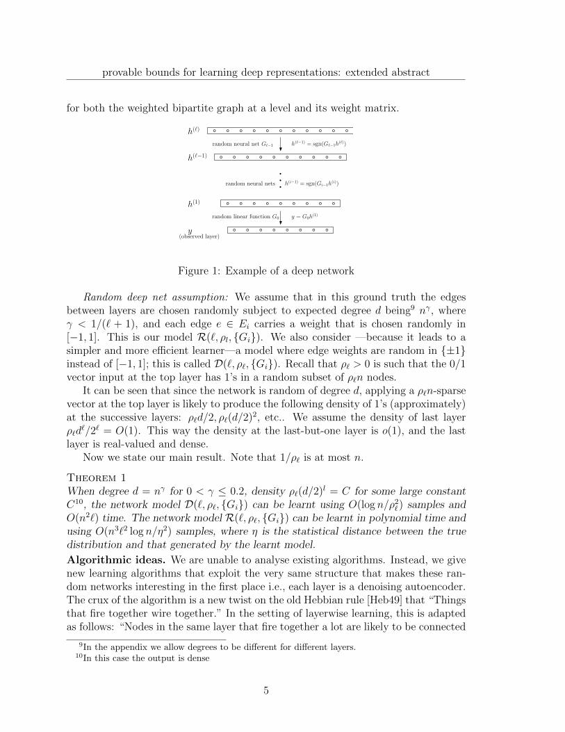
for both the weighted bipartite graph at a level and its weight matrix.
y
h(`−1)
h(1)
h(`)
random neural net G`−1
random linear function G0 y = G0h(1)
h(`−1) = sgn(G`−1h(`))
(observed layer)
random neural nets h(i−1) = sgn(Gi−1h(i))
Figure 1: Example of a deep network
Random deep net assumption: We assume that in this ground truth the edgesbetween layers are chosen randomly subject to expected degree d being9 nγ, whereγ < 1/(` + 1), and each edge e ∈ Ei carries a weight that is chosen randomly in[−1, 1]. This is our model R(`, ρl, Gi). We also consider —because it leads to asimpler and more efficient learner—a model where edge weights are random in ±1instead of [−1, 1]; this is called D(`, ρ`, Gi). Recall that ρ` > 0 is such that the 0/1vector input at the top layer has 1’s in a random subset of ρ`n nodes.
It can be seen that since the network is random of degree d, applying a ρ`n-sparsevector at the top layer is likely to produce the following density of 1’s (approximately)at the successive layers: ρ`d/2, ρ`(d/2)2, etc.. We assume the density of last layerρ`d
`/2` = O(1). This way the density at the last-but-one layer is o(1), and the lastlayer is real-valued and dense.
Now we state our main result. Note that 1/ρ` is at most n.
Theorem 1When degree d = nγ for 0 < γ ≤ 0.2, density ρ`(d/2)l = C for some large constantC10, the network model D(`, ρ`, Gi) can be learnt using O(log n/ρ2`) samples andO(n2`) time. The network model R(`, ρ`, Gi) can be learnt in polynomial time andusing O(n3`2 log n/η2) samples, where η is the statistical distance between the truedistribution and that generated by the learnt model.
Algorithmic ideas. We are unable to analyse existing algorithms. Instead, we givenew learning algorithms that exploit the very same structure that makes these ran-dom networks interesting in the first place i.e., each layer is a denoising autoencoder.The crux of the algorithm is a new twist on the old Hebbian rule [Heb49] that “Thingsthat fire together wire together.” In the setting of layerwise learning, this is adaptedas follows: “Nodes in the same layer that fire together a lot are likely to be connected
9In the appendix we allow degrees to be different for different layers.10In this case the output is dense
5
provable bounds for learning deep representations: extended abstract
(with positive weight) to the same node at the higher layer.” The algorithm consistsof looking for such pairwise (or 3-wise) correlations and putting together this infor-mation globally. The global procedure boils down to the graph-theoretic problemof reconstructing a bipartite graph given pairs of nodes that are at distance 2 in it(see Section 6). This is a variant of the GRAPH SQUARE ROOT problem which isNP-complete on worst-case instances but solvable for sparse random (or random-like)graphs.
Note that current algorithms (to the extent that they are Hebbian, roughly speak-ing) can also be seen as leveraging correlations. But putting together this informationis done via the language of nonlinear optimization (i.e., an objective function withsuitable penalty terms). Our ground truth network is indeed a particular local op-timum in any reasonable formulation. It would be interesting to show that existingalgorithms provably find the ground truth in polynomial time but currently this seemsdifficult.
Can our new ideas be useful in practice? We think that using a global reconstruc-tion procedure to leverage local correlations seems promising, especially if it avoidsthe usual nonlinear optimization. Our proof currently needs that the hidden layersare sparse, and the edge structure of the ground truth network is “random like”(inthe sense that two distinct features at a level tend to affect fairly disjoint-ish sets offeatures at the next level). Finally, we note that random neural nets do seem usefulin so-called reservoir computing, so perhaps they do provide useful representationalpower on real data. Such empirical study is left for future work.
Throughout, we need well-known properties of random graphs with expected de-gree d, such as the fact that they are expanders; these properties appear in theappendix. The most important one, unique neighbors property, appears in the nextSection.
3 Each layer is a Denoising Auto-encoder
As mentioned earlier, modern deep nets research often assumes that the net (or atleast some layers in it) should approximately preserve information, and even allowseasy going back/forth between representations in two adjacent layers (what we earliercalled “reversibility”). Below, y denotes the lower layer and h the higher (hidden)layer. Popular choices of s include logistic function, soft max, etc.; we use simplethreshold function in our model.
Definition 1 (Denoising autoencoder) An autoencoder consists of a decodingfunction D(h) = s(Wh+b) and an encoding function E(y) = s(W ′y+b′) where W,W ′
are linear transformations, b, b′ are fixed vectors and s is a nonlinear function thatacts identically on each coordinate. The autoencoder is denoising if E(D(h) + η) = hwith high probability where h is drawn from the distribution of the hidden layer, η is a
6
provable bounds for learning deep representations: extended abstract
noise vector drawn from the noise distribution, and D(h)+η is a shorthand for “D(h)corrupted with noise η.” The autoencoder is said to use weight tying if W ′ = W T .
In empirical work the denoising autoencoder property is only implicitly imposedon the deep net by minimizing the reconstruction error ||y−D(E(y+η))||, where η isthe noise vector. Our definition is slightly different but is actually stronger since y isexactly D(h) according to the generative model. Our definition implies the existenceof an encoder E that makes the penalty term exactly zero. We show that in ourground truth net (whether from model D(`, ρ`, Gi) or R(`, ρ`, Gi)) every pair ofsuccessive levels whp satisfies this definition, and with weight-tying.
We show a single-layer random network is a denoising autoencoder if the inputlayer is a random ρn sparse vector, and the output layer has density ρd/2 < 1/20.
Lemma 2If ρd < 0.1 (i.e., the assignment to the observed layer is also fairly sparse) then thesingle-layer network above is a denoising autoencoder with high probability (over thechoice of the random graph and weights), where the noise distribution is allowed toflip every output bit independently with probability 0.1. It uses weight tying.
The proof of this lemma highly relies on a property of random graph, called thestrong unique-neighbor property.
For any node u ∈ U and any subset S ⊂ U , let UF (u, S) be the sets of uniqueneighbors of u with respect to S,
UF (u, S) , v ∈ V : v ∈ F (u), v 6∈ F (S \ u)
Property 1 In a bipartite graph G(U, V,E,w), a node u ∈ U has (1 − ε)-uniqueneighbor property with respect to S if
∑
v∈UF (u,S)
|w(u, v)| ≥ (1− ε)∑
v∈F (u)
|w(u, v)| (1)
The set S has (1 − ε)-strong unique neighbor property if for every u ∈ U , u has(1− ε)-unique neighbor property with respect to S.
When we just assume ρd n, this property does not hold for all sets of size ρn.However, for any fixed set S of size ρn, this property holds with high probability overthe randomness of the graph.
Now we sketch the proof for Lemma 2 (details are in Appendix).For convenienceassume the edge weights are in −1, 1.
First, the decoder definition is implicit in our generative model: y = sgn(Wh).(That is, b = ~0 in the autoencoder definition.) Let the encoder be E(y) = sgn(W Ty+
7
provable bounds for learning deep representations: extended abstract
b′) for b′ = 0.2d×~1.In other words, the same bipartite graph and different thresholdscan transform an assignment on the lower level to the one at the higher level.
To prove this consider the strong unique-neighbor property of the network. Forthe set of nodes that are 1 at the higher level, a majority of their neighbors at thelower level are adjacent only to them and to no other nodes that are 1. The uniqueneighbors with a positive edge will always be 1 because there are no −1 edges thatcan cancel the +1 edge (similarly the unique neighbors with negative edge will alwaysbe 0). Thus by looking at the set of nodes that are 1 at the lower level, one can easilyinfer the correct 0/1 assignment to the higher level by doing a simple threshold of say0.2d at each node in the higher layer.
4 Learning a single layer network
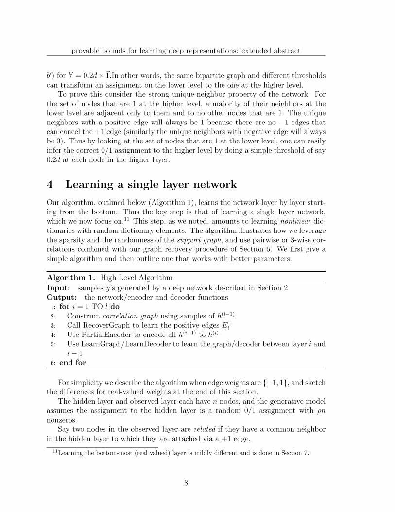
Our algorithm, outlined below (Algorithm 1), learns the network layer by layer start-ing from the bottom. Thus the key step is that of learning a single layer network,which we now focus on.11 This step, as we noted, amounts to learning nonlinear dic-tionaries with random dictionary elements. The algorithm illustrates how we leveragethe sparsity and the randomness of the support graph, and use pairwise or 3-wise cor-relations combined with our graph recovery procedure of Section 6. We first give asimple algorithm and then outline one that works with better parameters.
Algorithm 1. High Level Algorithm
Input: samples y’s generated by a deep network described in Section 2Output: the network/encoder and decoder functions
1: for i = 1 TO l do2: Construct correlation graph using samples of h(i−1)
3: Call RecoverGraph to learn the positive edges E+i
4: Use PartialEncoder to encode all h(i−1) to h(i)
5: Use LearnGraph/LearnDecoder to learn the graph/decoder between layer i andi− 1.
6: end for
For simplicity we describe the algorithm when edge weights are −1, 1, and sketchthe differences for real-valued weights at the end of this section.
The hidden layer and observed layer each have n nodes, and the generative modelassumes the assignment to the hidden layer is a random 0/1 assignment with ρnnonzeros.
Say two nodes in the observed layer are related if they have a common neighborin the hidden layer to which they are attached via a +1 edge.
11Learning the bottom-most (real valued) layer is mildly different and is done in Section 7.
8
provable bounds for learning deep representations: extended abstract
Step 1: Construct correlation graph: This step is a new twist on the classical Hebbianrule (“things that fire together wire together”).
Algorithm 2. PairwiseGraph
Input: N = O(log n/ρ) samples of y = sgn(Gh),Output: G on vertices V , u, v connected if related
for each u, v in the output layer doif ≥ ρN/3 samples have yu = yv = 1 then
connect u and v in Gend if
end for
Claim In a random sample of the output layer, related pairs u, v are both 1 withprobability at least 0.9ρ, while unrelated pairs are both 1 with probability at most(ρd)2.(Proof Sketch): First consider a related pair u, v, and let z be a vertex with +1 edgesto u, v. Let S be the set of neighbors of u, v excluding z. The size of S cannot bemuch larger than 2d. Under the choice of parameters, we know ρd 1, so the eventhS = ~0 conditioned on hz = 1 has probability at least 0.9. Hence the probability ofu and v being both 1 is at least 0.9ρ. Conversely, if u, v are unrelated then for bothu, v to be 1 there must be two different causes, namely, nodes y and z that are 1, andadditionally, are connected to u and v respectively via +1 edges. The chance of suchy, z existing in a random sparse assignment is at most (ρd)2 by union bound.
Thus, if ρ satisfies (ρd)2 < 0.1ρ, i.e., ρ < 0.1/d2, then using O(log n/ρ2) sampleswe can recover all related pairs whp, finishing the step.Step 2: Use graph recover procedure to find all edges that have weight +1. (SeeSection 6 for details.)Step 3: Using the +1 edges to encode all the samples y.
Algorithm 3. PartialEncoder
Input: positive edges E+, y = sgn(Gh), threshold θOutput: the hidden variable h
Let M be the indicator matrix of E+ (Mi,j = 1 iff (i, j) ∈ E+)return h = sgn(MTy − θ~1)
Although we have only recovered the positive edges, we can use PartialEncoderalgorithm to get h given y!
Lemma 3If support of h satisfies 11/12-strong unique neighbor property, and y = sgn(Gh),then Algorithm 3 outputs h with θ = 0.3d.
9
provable bounds for learning deep representations: extended abstract
This uses the unique neighbor property: for every z with hz = 1, it has at least0.4d unique neighbors that are connected with +1 edges. All these neighbors mustbe 1 so [(E+)Ty]z ≥ 0.4d. On the other hand, for any z with hz = 0, the uniqueneighbor property (applied to supp(h) ∪ z) implies that z can have at most 0.2dpositive edges to the +1’s in y. Hence h = sgn((E+)Ty − 0.3d~1).Step 4: Recover all weight −1 edges.
Algorithm 4. Learning Graph
Input: positive edges E+, samples of (h, y)Output: E−
1: R← (U × V ) \ E+.2: for each of the samples (h, y), and each v do3: Let S be the support of h4: if yv = 1 and S ∩B+(v) = u for some u then5: for s ∈ S do6: remove (s, v) from R.7: end for8: end if9: end for
10: return R
Now consider many pairs of (h, y), where h is found using Step 3. Suppose insome sample, yu = 1 for some u, and exactly one neighbor of u in the +1 edge graph(which we know entirely) is in supp(h). Then we can conclude that for any z withhz = 1, there cannot be a −1 edge (z, u), as this would cancel out the unique +1contribution.
Lemma 4Given O(log n/(ρ2d)) samples of pairs (h, y), with high probability (over the randomgraph and the samples) Algorithm 4 outputs the correct set E−.
To prove this lemma, we just need to bound the probability of the following eventfor any non-edge (x, u): hx = 1, |supp(h) ∩B+(u)| = 1, supp(h)∩B−(u) = ∅ (B+, B−
are positive and negative parents). These three events are almost independent, thefirst has probability ρ, second has probability ≈ ρd and the third has probabilityalmost 1.
Leveraging 3-wise correlation: The above sketch used pairwise correlations torecover the +1 weights when ρ < 1/d2, roughly. It turns out that using 3-wisecorrelations allow us to find correlations under a weaker requirement ρ < 1/d3/2.Now call three observed nodes u, v, s related if they are connected to a common nodeat the hidden layer via +1 edges. Then we can prove a claim analogous to the oneabove, which says that for a related triple, the probability that u, v, s are all 1 is at
10
provable bounds for learning deep representations: extended abstract
least 0.9ρ, while the probability for unrelated triples is roughly at most (ρd)3. Thusas long as ρ < 0.1/d3/2, it is possible to find related triples correctly. The graphrecover algorithm can be modified to run on 3-uniform hypergraph consisting ofthese related triples to recover the +1 edges.
The end result is the following theorem. This is the learner used to get the boundsstated in our main theorem.
Theorem 5Suppose our generative neural net model with weights −1, 1 has a single layer and
the assignment of the hidden layer is a random ρn-sparse vector, with ρ 1/d3/2.Then there is an algorithm that runs in O(n(d3 + n)) time and uses O(log n/ρ2)samples to recover the ground truth with high probability over the randomness of thegraph and the samples.
When weights are real numbers. We only sketch this and leave the details tothe appendix. Surprisingly, steps 1, 2 and 3 still work. In the proofs, we have onlyused the sign of the edge weights – the magnitude of the edge weights can be arbitrary.This is because the proofs in these steps relies on the unique neighbor property, ifsome node is on (has value 1), then its unique positive neighbors at the next levelwill always be on, no matter how small the positive weights might be. Also notice inPartialEncoder we are only using the support of E+, but not the weights.
After Step 3 we have turned the problem of unsupervised learning of the hiddengraph to a supervised one in which the outputs are just linear classifiers over theinputs! Thus the weights on the edges can be learnt to any desired accuracy.
5 Correlations in a Multilayer Network
We now consider multi-layer networks, and show how they can be learnt layerwiseusing a slight modification of our one-layer algorithm at each layer. At a technicallevel, the difficulty in the analysis is the following: in single-layer learning, we as-sumed that the higher layer’s assignment is a random ρn-sparse binary vector. Inthe multilayer network, the assignments in intermediate layers (except for the toplayer) do not satisfy this, but we will show that the correlations among them arelow enough that we can carry forth the argument. Again for simplicity we describethe algorithm for the model D(`, ρl, Gi), in which the edge weights are ±1. Alsoto keep notation simple, we describe how to bound the correlations in bottom-mostlayer (h(1)). It holds almost verbatim for the higher layers. We define ρi to be the“expected” number of 1s in the layer h(i). Because of the unique neighbor property,we expect roughly ρl(d/2) fraction of h(`−1) to be 1. So also, for subsequent layers,we obtain ρi = ρ` · (d/2)`−i. (We can also think of the above expression as definingρi).
11
provable bounds for learning deep representations: extended abstract
Lemma 6Consider a network from D(`, ρl, Gi). With high probability (over the random
graphs between layers) for any two nodes u, v in layer h(1),
Pr[h(1)u = h(1)v = 1]
≥ ρ2/2 if u, v related≤ ρ2/4 otherwise
Proof:(outline) The first step is to show that for a vertex u in level i, Pr[h(i)(u) = 1]is at least 3ρi/4 and at most 5ρi/4. This is shown by an inductive argument (detailsin the full version). (This is the step where we crucially use the randomness of theunderlying graph.)
Now suppose u, v have a common neighbor z with +1 edges to both of them.Consider the event that z is 1 and none of the neighbors of u, v with −1 weight edgesare 1 in layer h(2). These conditions ensure that h(1)(u) = h(1)(v) = 1; further, theyturn out to occur together with probability at least ρ2/2, because of the bound fromthe first step, along with the fact that u, v combined have only 2d neighbors (and2dρ2n n), so there is good probability of not picking neighbors with −1 edges.
If u, v are not related, it turns out that the probability of interest is at most 2ρ21plus a term which depends on whether u, v have a common parent in layer h(3) in thegraph restricted to +1 edges. Intuitively, picking one of these common parents couldresult in u, v both being 1. By our choice of parameters, we will have ρ21 < ρ2/20, andalso the additional term will be < ρ2/10, which implies the desired conclusion. 2
Then as before, we can use graph recovery to find all the +1 edges in the graphat the bottom most layer. This can then be used (as in Step 3) in the single layeralgorithm to encode h(1) and obtain values for h(2). Now as before, we have manypairs (h(2), h(1)), and thus using precisely the reasoning of Step 4 earlier, we can obtainthe full graph at the bottom layer.
This argument can be repeated after ‘peeling off’ the bottom layer, thus allowingus to learn layer by layer.
6 Graph Recovery
Graph reconstruction consists of recovering a graph given information about its sub-graphs [BH77]. A prototypical problem is the Graph Square Root problem, whichcalls for recovering a graph given all pairs of nodes whose distance is at most 2. Thisis NP-hard.
Definition 2 (Graph Recovery) Let G1(U, V,E1) be an unknown random bipar-tite graph between |U | = n and |V | = n vertices where each edge is picked withprobability d/n independently.Given: Graph G(V,E) where (v1, v2) ∈ E iff v1 and v2 share a common parent in G1
(i.e. ∃u ∈ U where (u, v1) ∈ E1 and (u, v2) ∈ E1).Goal: Find the bipartite graph G1.
12
provable bounds for learning deep representations: extended abstract
Some of our algorithms (using 3-wise correlations) need to solve analogous problemwhere we are given triples of nodes which are mutually at distance 2 from each other,which we will not detail for lack of space.
We let F (S) (resp. B(S)) denote the set of neighbors of S ⊆ U (resp. ⊆ V ) in G1.Also Γ(·) gives the set of neighbors in G. Now for the recovery algorithm to work, weneed the following properties (all satisfied whp by random graph when d3/n 1):
1. For any v1, v2 ∈ V ,|(Γ(v1) ∩ Γ(v2))\(F (B(v1) ∩B(v2)))| < d/20.
2. For any u1, u2 ∈ U , |F (u1) ∪ F (u2)| > 1.5d.
3. For any u ∈ U , v ∈ V and v 6∈ F (u), |Γ(v) ∩ F (u)| < d/20.
4. For any u ∈ U , at least 0.1 fraction of pairs v1, v2 ∈ F (u) does not have acommon neighbor other than u.
The first property says “most correlations are generated by common cause”: allbut possibly d/20 of the common neighbors of v1 and v2 in G, are in fact neighborsof a common neighbor of v1 and v2 in G1.
The second property basically says the sets F (u)’s should be almost disjoint, thisis clear because the sets are chosen at random.
The third property says if a vertex v is not related to the cause u, then it cannothave correlation with all many neighbors of u.
The fourth property says every cause introduces a significant number of correla-tions that is unique to that cause.
In fact, Properties 2-4 are closely related from the unique neighbor property.
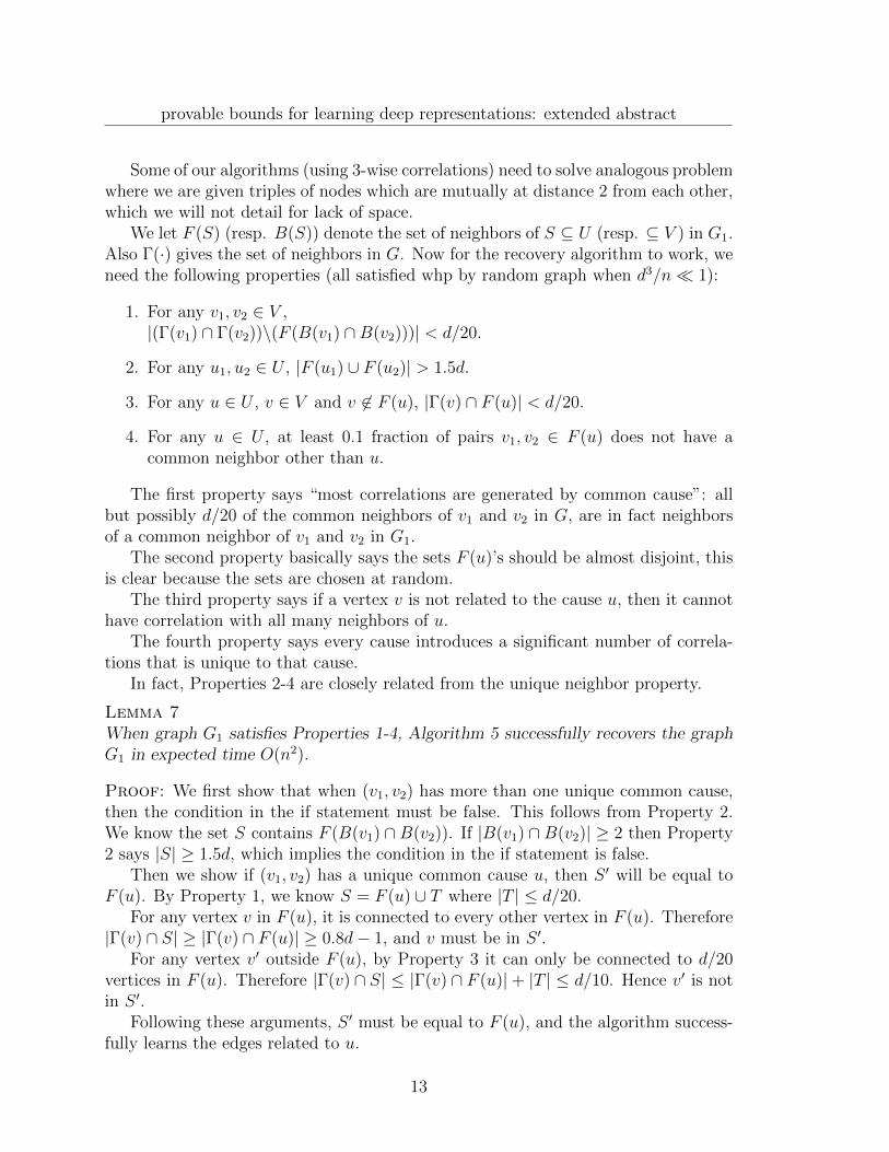
Lemma 7When graph G1 satisfies Properties 1-4, Algorithm 5 successfully recovers the graphG1 in expected time O(n2).
Proof: We first show that when (v1, v2) has more than one unique common cause,then the condition in the if statement must be false. This follows from Property 2.We know the set S contains F (B(v1) ∩B(v2)). If |B(v1) ∩B(v2)| ≥ 2 then Property2 says |S| ≥ 1.5d, which implies the condition in the if statement is false.
Then we show if (v1, v2) has a unique common cause u, then S ′ will be equal toF (u). By Property 1, we know S = F (u) ∪ T where |T | ≤ d/20.
For any vertex v in F (u), it is connected to every other vertex in F (u). Therefore|Γ(v) ∩ S| ≥ |Γ(v) ∩ F (u)| ≥ 0.8d− 1, and v must be in S ′.
For any vertex v′ outside F (u), by Property 3 it can only be connected to d/20vertices in F (u). Therefore |Γ(v) ∩ S| ≤ |Γ(v) ∩ F (u)|+ |T | ≤ d/10. Hence v′ is notin S ′.
Following these arguments, S ′ must be equal to F (u), and the algorithm success-fully learns the edges related to u.
13
provable bounds for learning deep representations: extended abstract
The algorithm will successfully find all vertices u ∈ U because of Property 4: forevery u there are enough number of edges in G that is only caused by u. When oneof them is sampled, the algorithm successfully learns the vertex u.
Finally we bound the running time. By Property 4 we know that the algorithmidentifies a new vertex u ∈ U in at most 10 iterations in expectation. Each iterationtakes at most O(n) time. Therefore the algorithm takes at most O(n2) time inexpectation. 2
Algorithm 5. RecoverGraph
Input: G given as in Definition 2Output: Find the graph G1 as in Definition 2.
repeatPick a random edge (v1, v2) ∈ E.Let S = v : (v, v1), (v, v2) ∈ E.if |S| < 1.3d thenS ′ = v ∈ S : |Γ(v) ∩ S| ≥ 0.8d− 1 S ′ should be a clique in GIn G1, create a vertex u and connect u to every v ∈ S ′.Mark all the edges (v1, v2) for v1, v2 ∈ S ′.
end ifuntil all edges are marked
7 Learning the lowermost (real-valued) layer
Note that in our model, the lowest (observed) layer is real-valued and does not havethreshold gates. Thus our earlier learning algorithm cannot be applied as is. However,we see that the same paradigm – identifying correlations and using Graph recover– can be used.
The first step is to show that for a random weighted graph G, the linear decoderD(h) = Gh and the encoder E(y) = sgn(GTy+ b) form a denoising autoencoder withreal-valued outputs, as in Bengio et al. [BCV13].
Lemma 8If G is a random weighted graph, the encoder E(y) = sgn(GTy − 0.4d~1) and lineardecoder D(h) = Gh form a denoising autoencoder, for noise vectors γ which haveindependent components, each having variance at most O(d/ log2 n).
The next step is to show a bound on correlations as before. For simplicity westate it assuming the layer h(1) has a random 0/1 assignment of sparsity ρ1. In thefull version we state it keeping in mind the higher layers, as we did in the previoussections.
14
provable bounds for learning deep representations: extended abstract
Theorem 9When ρ1d = O(1), d = Ω(log2 n), with high probability over the choice of the weightsand the choice of the graph, for any three nodes u, v, s the assignment y to the bottomlayer satisfies:
1. If u, v and s have no common neighbor, then |Eh[yuyvys]| ≤ ρ1/3
2. If u, v and s have a unique common neighbor, then |Eh[yuyvys]| ≥ 2ρ1/3
8 Two layers cannot be represented by one layer
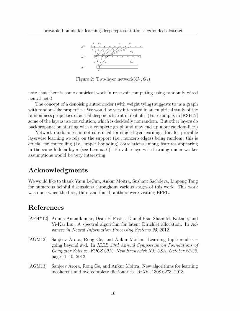
In this section we show that a two-layer network with ±1 weights is more expressivethan one layer network with arbitrary weights. A two-layer network (G1, G2) consistsof random graphs G1 and G2 with random ±1 weights on the edges. Viewed asa generative model, its input is h(3) and the output is h(1) = sgn(G1 sgn(G2h
(3))).We will show that a single-layer network even with arbitrary weights and arbitrarythreshold functions must generate a fairly different distribution.
Lemma 10For almost all choices of (G1, G2), the following is true. For every one layer net-
work with matrix A and vector b, if h(3) is chosen to be a random ρ3n-sparse vectorwith ρ3d2d1 1, the probability (over the choice of h(3)) is at least Ω(ρ23) thatsgn(G1 sgn(G1h
(3))) 6= sgn(Ah(3) + b).
The idea is that the cancellations possible in the two-layer network simply cannotall be accomodated in a single-layer network even using arbitrary weights. Moreprecisely, even the bit at a single output node v cannot be well-represented by asimple threshold function.
First, observe that the output at v is determined by values of d1d2 nodes at thetop layer that are its ancestors. It is not hard to show in the one layer net (A, b),there should be no edge between v and any node u that is not its ancestor. Thenconsider structure in Figure 2. Assuming all other parents of v are 0 (which happenwith probability at least 0.9), and focus on the values of (u1, u2, u3, u4). When thesevalues are (1, 1, 0, 0) and (0, 0, 1, 1), v is off. When these values are (1, 0, 0, 1) and(0, 1, 1, 0), v is on. This is impossible for a one layer network because the first twoask for
∑Aui,v
+2bv ≤ 0 and the second two ask for∑
Aui,v+2bv < 0.
9 Conclusions
Rigorous analysis of interesting subcases of any ML problem can be beneficial fortriggering further improvements: see e.g., the role played in Bayes nets by the rigorousanalysis of message-passing algorithms for trees and graphs of low tree-width. This isthe spirit in which to view our consideration of a random neural net model (though
15
provable bounds for learning deep representations: extended abstract
h(1)
h(2)
v
+1 -1
+1
u1 u2 u3h(3)
+1
+1
G2
G1
s s′
u4
-1
Figure 2: Two-layer network(G1, G2)
note that there is some empirical work in reservoir computing using randomly wiredneural nets).
The concept of a denoising autoencoder (with weight tying) suggests to us a graphwith random-like properties. We would be very interested in an empirical study of therandomness properties of actual deep nets learnt in real life. (For example, in [KSH12]some of the layers use convolution, which is decidedly nonrandom. But other layers dobackpropagation starting with a complete graph and may end up more random-like.)
Network randomness is not so crucial for single-layer learning. But for provablelayerwise learning we rely on the support (i.e., nonzero edges) being random: this iscrucial for controlling (i.e., upper bounding) correlations among features appearingin the same hidden layer (see Lemma 6). Provable layerwise learning under weakerassumptions would be very interesting.
Acknowledgments
We would like to thank Yann LeCun, Ankur Moitra, Sushant Sachdeva, Linpeng Tangfor numerous helpful discussions throughout various stages of this work. This workwas done when the first, third and fourth authors were visiting EPFL.
References
[AFH+12] Anima Anandkumar, Dean P. Foster, Daniel Hsu, Sham M. Kakade, andYi-Kai Liu. A spectral algorithm for latent Dirichlet allocation. In Ad-vances in Neural Information Processing Systems 25, 2012.
[AGM12] Sanjeev Arora, Rong Ge, and Ankur Moitra. Learning topic models –going beyond svd. In IEEE 53rd Annual Symposium on Foundations ofComputer Science, FOCS 2012, New Brunswick NJ, USA, October 20-23,pages 1–10, 2012.
[AGM13] Sanjeev Arora, Rong Ge, and Ankur Moitra. New algorithms for learningincoherent and overcomplete dictionaries. ArXiv, 1308.6273, 2013.
16

provable bounds for learning deep representations: extended abstract
[BCV13] Yoshua Bengio, Aaron C. Courville, and Pascal Vincent. Representationlearning: A review and new perspectives. IEEE Trans. Pattern Anal.Mach. Intell., 35(8):1798–1828, 2013.
[Ben09] Yoshua Bengio. Learning deep architectures for AI. Foundations andTrends in Machine Learning, 2(1):1–127, 2009. Also published as a book.Now Publishers, 2009.
[BGI+08] R. Berinde, A.C. Gilbert, P. Indyk, H. Karloff, and M.J. Strauss. Com-bining geometry and combinatorics: a unified approach to sparse signalrecovery. In 46th Annual Allerton Conference on Communication, Con-trol, and Computing, pages 798–805, 2008.
[BH77] J Adrian Bondy and Robert L Hemminger. Graph reconstructiona survey.Journal of Graph Theory, 1(3):227–268, 1977.
[CS09] Youngmin Cho and Lawrence Saul. Kernel methods for deep learning. InAdvances in Neural Information Processing Systems 22, pages 342–350.2009.
[Don06] David L Donoho. Compressed sensing. Information Theory, IEEE Trans-actions on, 52(4):1289–1306, 2006.
[Heb49] Donald O. Hebb. The Organization of Behavior: A NeuropsychologicalTheory. Wiley, new edition edition, June 1949.
[HK13] Daniel Hsu and Sham M. Kakade. Learning mixtures of spherical gaus-sians: moment methods and spectral decompositions. In Proceedings ofthe 4th conference on Innovations in Theoretical Computer Science, pages11–20, 2013.
[HKZ12] Daniel Hsu, Sham M. Kakade, and Tong Zhang. A spectral algorithmfor learning hidden Markov models. Journal of Computer and SystemSciences, 78(5):1460–1480, 2012.
[JKS02] Jeffrey C Jackson, Adam R Klivans, and Rocco A Servedio. Learnabilitybeyond ac0. In Proceedings of the thiry-fourth annual ACM symposiumon Theory of computing, pages 776–784. ACM, 2002.
[KS09] Adam R Klivans and Alexander A Sherstov. Cryptographic hardnessfor learning intersections of halfspaces. Journal of Computer and SystemSciences, 75(1):2–12, 2009.
[KSH12] Alex Krizhevsky, Ilya Sutskever, and Geoff Hinton. Imagenet classifi-cation with deep convolutional neural networks. In Advances in NeuralInformation Processing Systems 25, pages 1106–1114. 2012.
17
provable bounds for learning deep representations: extended abstract
[LSSS13] Roi Livni, Shai Shalev-Shwartz, and Ohad Shamir. A provably efficientalgorithm for training deep networks. ArXiv, 1304.7045, 2013.
[MV10] Ankur Moitra and Gregory Valiant. Settling the polynomial learnability ofmixtures of gaussians. In the 51st Annual Symposium on the Foundationsof Computer Science (FOCS), 2010.
[VLBM08] Pascal Vincent, Hugo Larochelle, Yoshua Bengio, and Pierre-AntoineManzagol. Extracting and composing robust features with denoising au-toencoders. In ICML, pages 1096–1103, 2008.
18
Provable Bounds for Learning Some DeepRepresentations: Long Technical Appendix∗
Sanjeev Arora Aditya Bhaskara Rong Ge Tengyu Ma
A Preliminaries and Notations
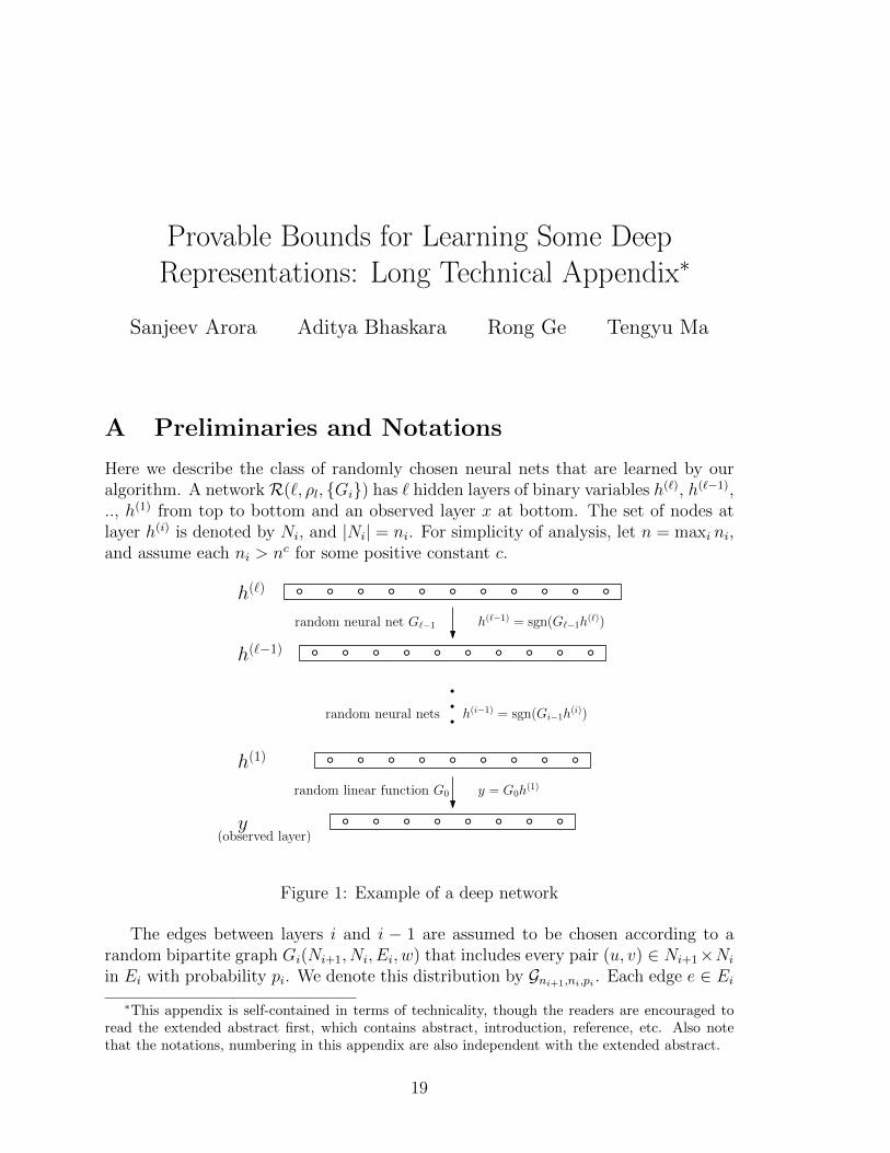
Here we describe the class of randomly chosen neural nets that are learned by ouralgorithm. A networkR(`, ρl, Gi) has ` hidden layers of binary variables h(`), h(`−1),.., h(1) from top to bottom and an observed layer x at bottom. The set of nodes atlayer h(i) is denoted by Ni, and |Ni| = ni. For simplicity of analysis, let n = maxi ni,and assume each ni > nc for some positive constant c.
y
h(`−1)
h(1)
h(`)
random neural net G`−1
random linear function G0 y = G0h(1)
h(`−1) = sgn(G`−1h(`))
(observed layer)
random neural nets h(i−1) = sgn(Gi−1h(i))
Figure 1: Example of a deep network
The edges between layers i and i − 1 are assumed to be chosen according to arandom bipartite graph Gi(Ni+1, Ni, Ei, w) that includes every pair (u, v) ∈ Ni+1×Ni
in Ei with probability pi. We denote this distribution by Gni+1,ni,pi . Each edge e ∈ Ei∗This appendix is self-contained in terms of technicality, though the readers are encouraged to
read the extended abstract first, which contains abstract, introduction, reference, etc. Also notethat the notations, numbering in this appendix are also independent with the extended abstract.
19
provable bounds for learning deep representations: technical appendix
carries a weight w(e) in [−1, 1] that is randomly chosen.The set of positive edges aredenoted by E+
i = (u, v) ∈ Ni+1 × Ni : w(u, v) > 0. Define E− to be the negativeedges similarly. Denote by G+ and G− the corresponding graphs defined by E+ andE−, respectively.
The generative model works like a neural net where the threshold at every nodeis 0. The top layer h(`) is initialized a 0/1 assignment where the set of nodes that are1 is picked uniformly among all sets of size ρlnl. Each node in layer `− 1 computes aweighted sum of its neighbors in layer `, and becomes 1 iff that sum strictly exceeds0. We will use sgn(·) to denote the threshold function:
sgn(x) = 1 if x > 0 and 0 else. (1)
Applying sgn() to a vector involves applying it componentwise. Thus the networkcomputes as follows: h(i−1) = sgn(Gi−1h
(i)) for all i > 0 and h(0) = G0h(1) (i.e., no
threshold at the observed layer)1. Here (with slight abuse of notation) Gi stands forboth the bipartite graph and the bipartite weight matrix of the graph at layer i.
We also consider a simpler case when the edge weights are in ±1 instead of[−1, 1]. We call such a network D(`, ρl, Gi).
Throughout this paper, by saying “with high probability” we mean the probabilityis at least 1−n−C for some large constant C. Moreover, f g means f ≥ Cg , f gmeans f ≤ g/C for large enough constant C (the constant required is determinedimplicitly by the related proofs).
More network notations. The expected degree from Ni to Ni+1 is di, that is,di , pi|Ni+1| = pini+1, and the expected degree from Ni+1 to Ni is denoted byd′i , pi|Ni| = pini. The set of forward neighbors of u ∈ Ni+1 in graph Gi is denotedby Fi(u) = v ∈ Ni : (u, v) ∈ Ei, and the set of backward neighbors of v ∈ Ni in Gi
is denoted by Bi(v) = u ∈ Ni+1 : (u, v) ∈ Ei. We use F+i (u) to denote the positive
neighbors: F+i (u) , v, : (u, v) ∈ E+
i (and similarly for B+i (v)). The expected
density of the layers are defined as ρi−1 = ρidi−1/2 (ρ` is given as a parameter of themodel).
Our analysis works while allowing network layers of different sizes and differentdegrees. For simplicity, we recommend first-time readers to assume all the ni’s areequal, and di = d′i for all layers.
Basic facts about random graphs We will assume that in our random graphsthe expected degree d′, d log n so that most events of interest to us that happen inexpectation actually happen with high probability (see Appendix J): e.g., all hiddennodes have backdegree d±√d log n. Of particular interest will be the fact (used often
1We can also allow the observed layer to also use threshold but then our proof requires the outputvector to be somewhat sparse. This could be meaningful in modeling practical settings where eachdatapoint has been represented as a somewhat sparse 0/1 vector via a sparse coding algorithm.
20
provable bounds for learning deep representations: technical appendix
in theoretical computer science) that random bipartite graphs have a unique neighborproperty. This means that every set of nodes S on one layer has |S| (d′ ± o(d′))neighbors on the neighboring layer provided |S| d′ n, which implies in particularthat most of these neighboring nodes are adjacent to exactly one node in S: theseare called unique neighbors. We will need a stronger version of unique neighborsproperty which doesn’t hold for all sets but holds for every set with probability atleast 1 − exp(−d′) (over the choice of the graph). It says that every node that isnot in S shares at most (say) 0.1d′ neighbors with any node in S. This is crucial forshowing that each layer is a denoising autoencoder.
B Main Results
In this paper, we give an algorithm that learns a random deep neural network.
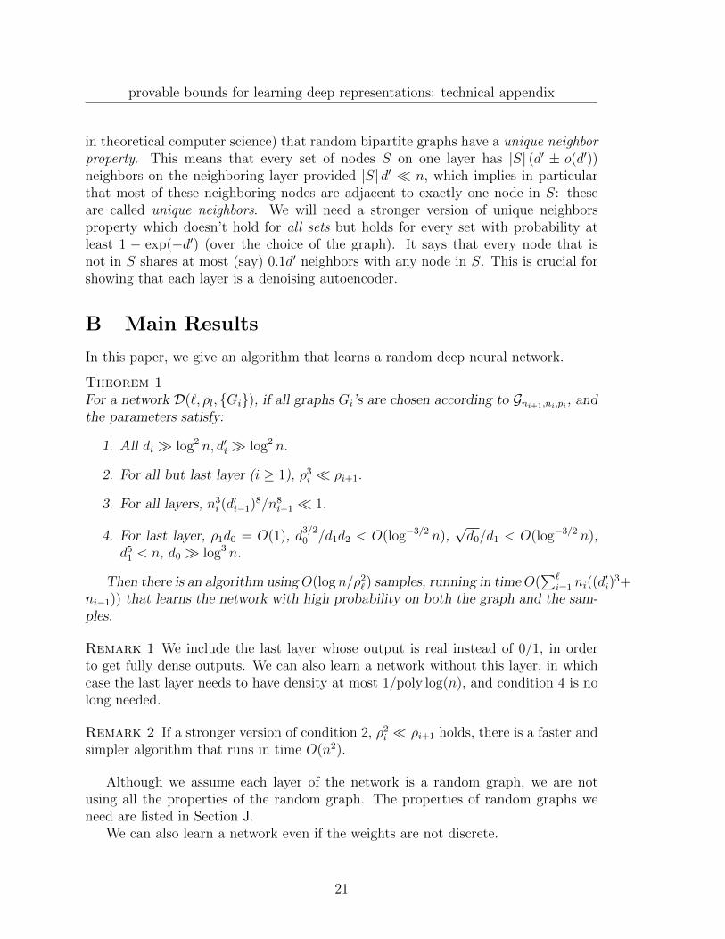
Theorem 1For a network D(`, ρl, Gi), if all graphs Gi’s are chosen according to Gni+1,ni,pi , andthe parameters satisfy:
1. All di log2 n, d′i log2 n.
2. For all but last layer (i ≥ 1), ρ3i ρi+1.
3. For all layers, n3i (d′i−1)8/n8
i−1 1.
4. For last layer, ρ1d0 = O(1), d3/20 /d1d2 < O(log−3/2 n),
√d0/d1 < O(log−3/2 n),
d51 < n, d0 log3 n.
Then there is an algorithm usingO(log n/ρ2`) samples, running in timeO(
∑`i=1 ni((d
′i)
3+ni−1)) that learns the network with high probability on both the graph and the sam-ples.
Remark 1 We include the last layer whose output is real instead of 0/1, in orderto get fully dense outputs. We can also learn a network without this layer, in whichcase the last layer needs to have density at most 1/poly log(n), and condition 4 is nolong needed.
Remark 2 If a stronger version of condition 2, ρ2i ρi+1 holds, there is a faster and
simpler algorithm that runs in time O(n2).
Although we assume each layer of the network is a random graph, we are notusing all the properties of the random graph. The properties of random graphs weneed are listed in Section J.
We can also learn a network even if the weights are not discrete.
21
provable bounds for learning deep representations: technical appendix
Theorem 2For a network R(`, ρl, Gi), if all graphs Gi’s are chosen according to Gni+1,ni,pi , andthe parameters satisfy the same conditions as in Theorem 1, there is an algorithmusing O(n2
l nl−1l2 log n/η2) samples, running in time poly(n) that learns a network
R′(`, ρl, G′i). The observed vectors of network R′ agrees with R(`, ρl, Gi) on(1− η) fraction of the hidden variable h(l).
C Each layer is a Denoising Auto-encoder
Experts feel that deep networks satisfy some intuitive properties. First, intermediatelayers in a deep representation should approximately preserve the useful informationin the input layer. Next, it should be possible to go back/forth easily between therepresentations in two successive layers, and in fact they should be able to use theneural net itself to do so. Finally, this process of translating between layers should benoise-stable to small amounts of random noise. All this was implicit in the early workon RBM and made explicit in the paper of Vincent et al. [VLBM08] on denoisingautoencoders. For a theoretical justification of the notion of a denoising autoencoderbased upon the ”manifold assumption” of machine learning see the survey of Ben-gio [Ben09].
Definition 1 (Denoising autoencoder) An autoencoder consists of an decod-ing function D(h) = s(Wh + b) and a encoding function E(y) = s(W ′y + b′) whereW,W ′ are linear transformations, b, b′ are fixed vectors and s is a nonlinear functionthat acts identically on each coordinate. The autoencoder is denoising if E(D(h)+η) =h with high probability where h is drawn from the input distribution, η is a noise vectordrawn from the noise distribution, and D(h) + η is a shorthand for “E(h) corruptedwith noise η.” The autoencoder is said to use weight tying if W ′ = W T .
The popular choices of s includes logistic function, soft max, etc. In this work wechoose s to be a simple threshold on each coordinate (i.e., the test > 0, this can beviewed as an extreme case of logistic function). Weight tying is a popular constraintand is implicit in RBMs. Our work also satisfies weight tying.
In empirical work the denoising autoencoder property is only implicitly imposedon the deep net by minimizing the reconstruction error ||y − D(E(y))||, where y isa corrupted version of y; our definition is very similar in spirit that it also enforcesthe noise-stability of the autoencoder in a stronger sense. It actually implies that thereconstruction error corresponds to the noise from y, which is indeed small. We showthat in our ground truth net (whether from model D(`, ρ`, Gi) or R(`, ρ`, Gi))every pair of successive levels whp satisfies this definition, and with weight-tying.
We will show that each layer of our network is a denoising autoencoder with veryhigh probability. (Each layer can also be viewed as an RBM with an additional energyterm to ensure sparsity of h.) Later we will of course give efficient algorithms to learn
22
provable bounds for learning deep representations: technical appendix
such networks without recoursing to local search. In this section we just prove theysatisfy Definition 1.
The single layer has m hidden and n output (observed) nodes. The connectiongraph between them is picked randomly by selecting each edge independently withprobability p and putting a random weight on it in [−1, 1]. Then the linear transfor-mation W corresponds simply to this matrix of weights. In our autoencoder we setb = ~0 and b′ = 0.2d′ × ~1, where d′ = pn is the expected degree of the random graphon the hidden side. (By simple Chernoff bounds, every node has degree very close tod′.) The hidden layer h has the following prior: it is given a 0/1 assignment that is1 on a random subset of hidden nodes of size ρm. This means the number of nodesin the output layer that are 1 is at most ρmd′ = ρnd, where d = pm is the expecteddegree on the observed side. We will see that since b = ~0 the number of nodes thatare 1 in the output layer is close to ρmd′/2.
Lemma 3If ρmd′ < 0.05n (i.e., the assignment to the observed layer is also fairly sparse) thenthe single-layer network above is a denoising autoencoder with high probability (overthe choice of the random graph and weights), where the noise distribution is allowedto flip every output bit independently with probability 0.01.
Remark: The parameters accord with the usual intuition that the information contentmust decrease when going from observed layer to hidden layer.Proof: By definition, D(h) = sgn(Wh). Let’s understand what D(h) looks like. IfS is the subset of nodes in the hidden layer that are 1 in h, then the unique neighborproperty (Corollary 30) implies that (i) With high probability each node u in S hasat least 0.9d′ neighboring nodes in the observed layer that are neighbors to no othernode in S. Furthermore, at least 0.44d′ of these are connected to u by a positive edgeand 0.44d′ are connected by a negative edge. All 0.44d′ of the former nodes musttherefore have a value 1 in D(h). Furthermore, it is also true that the total weightof these 0.44d′ positive edges is at least 0.21d′. (ii) Each v not in S has at most 0.1d′
neighbors that are also neighbors of any node in S.Now let’s understand the encoder, specifically, E(D(h)). It assigns 1 to a node in
the hidden layer iff the weighted sum of all nodes adjacent to it is at least 0.2d′. By(i), every node in S must be set to 1 in E(D(h)) and no node in S is set to 1. ThusE(D(h)) = h for most h’s and we have shown that the autoencoder works correctly.Furthermore, there is enough margin that the decoding stays stable when we flip 0.01fraction of bits in the observed layer. 2
D Learning a single layer network
We first consider the question of learning a single layer network, which as notedamounts to learning nonlinear dictionaries. It perfectly illustrates how we leveragethe sparsity and the randomness of the support graph.
23
provable bounds for learning deep representations: technical appendix
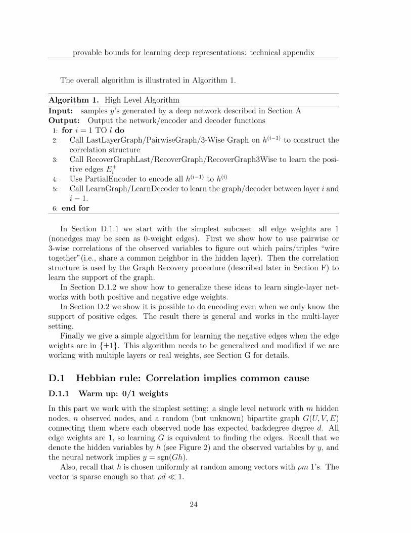
The overall algorithm is illustrated in Algorithm 1.
Algorithm 1. High Level Algorithm
Input: samples y’s generated by a deep network described in Section AOutput: Output the network/encoder and decoder functions
1: for i = 1 TO l do2: Call LastLayerGraph/PairwiseGraph/3-Wise Graph on h(i−1) to construct the
correlation structure3: Call RecoverGraphLast/RecoverGraph/RecoverGraph3Wise to learn the posi-
tive edges E+i
4: Use PartialEncoder to encode all h(i−1) to h(i)
5: Call LearnGraph/LearnDecoder to learn the graph/decoder between layer i andi− 1.
6: end for
In Section D.1.1 we start with the simplest subcase: all edge weights are 1(nonedges may be seen as 0-weight edges). First we show how to use pairwise or3-wise correlations of the observed variables to figure out which pairs/triples “wiretogether”(i.e., share a common neighbor in the hidden layer). Then the correlationstructure is used by the Graph Recovery procedure (described later in Section F) tolearn the support of the graph.
In Section D.1.2 we show how to generalize these ideas to learn single-layer net-works with both positive and negative edge weights.
In Section D.2 we show it is possible to do encoding even when we only know thesupport of positive edges. The result there is general and works in the multi-layersetting.
Finally we give a simple algorithm for learning the negative edges when the edgeweights are in ±1. This algorithm needs to be generalized and modified if we areworking with multiple layers or real weights, see Section G for details.
D.1 Hebbian rule: Correlation implies common cause
D.1.1 Warm up: 0/1 weights
In this part we work with the simplest setting: a single level network with m hiddennodes, n observed nodes, and a random (but unknown) bipartite graph G(U, V,E)connecting them where each observed node has expected backdegree degree d. Alledge weights are 1, so learning G is equivalent to finding the edges. Recall that wedenote the hidden variables by h (see Figure 2) and the observed variables by y, andthe neural network implies y = sgn(Gh).
Also, recall that h is chosen uniformly at random among vectors with ρm 1’s. Thevector is sparse enough so that ρd 1.
24
provable bounds for learning deep representations: technical appendix
y
h
G
(observed layer)
(hidden layer)
s u v
z
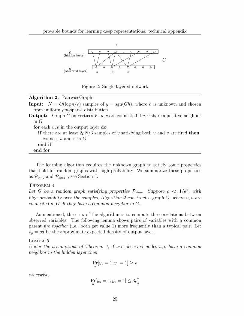
Figure 2: Single layered network
Algorithm 2. PairwiseGraph
Input: N = O(log n/ρ) samples of y = sgn(Gh), where h is unknown and chosenfrom uniform ρm-sparse distribution
Output: Graph G on vertices V , u, v are connected if u, v share a positive neighborin Gfor each u, v in the output layer do
if there are at least 2ρN/3 samples of y satisfying both u and v are fired thenconnect u and v in G
end ifend for
The learning algorithm requires the unknown graph to satisfy some propertiesthat hold for random graphs with high probability. We summarize these propertiesas Psing and Psing+, see Section J.
Theorem 4Let G be a random graph satisfying properties Psing. Suppose ρ 1/d2, with
high probability over the samples, Algorithm 2 construct a graph G, where u, v areconnected in G iff they have a common neighbor in G.
As mentioned, the crux of the algorithm is to compute the correlations betweenobserved variables. The following lemma shows pairs of variables with a commonparent fire together (i.e., both get value 1) more frequently than a typical pair. Letρy = ρd be the approximate expected density of output layer.
Lemma 5Under the assumptions of Theorem 4, if two observed nodes u, v have a commonneighbor in the hidden layer then
Prh
[yu = 1, yv = 1] ≥ ρ
otherwise,Prh
[yu = 1, yv = 1] ≤ 3ρ2y
25
provable bounds for learning deep representations: technical appendix
Proof: When u and v has a common neighbor z in the input layer, as long as z isfired both u and v are fired. Thus Pr[yu = 1, yv = 1] ≥ Pr[hz = 1] = ρ.
On the other hand, suppose the neighbor of u (B(u)) and the neighbors of v (B(v))are disjoint. Since yu = 1 only if the support of h intersect with the neighbors of u,we have Pr[yu = 1] = Pr[supp(h) ∩ B(u) 6= ∅]. Similarly, we know Pr[yu = 1, yv =1] = Pr[supp(h) ∩B(u) 6= ∅, supp(h) ∩B(v) 6= ∅].
Note that under assumptions Psing B(u) andB(v) have size at most 1.1d. Lemma 38implies Pr[supp(h) ∩B(u) 6= ∅, supp(h) ∩B(u) 6= ∅] ≤ 2ρ2|B(u)| · |B(v)| ≤ 3ρ2
y. 2
The lemma implies that when ρ2y ρ(which is equivalent to ρ 1/(d2)), we can
find pairs of nodes with common neighbors by estimating the probability that theyare both 1.
In order to prove Theorem 4 from Lemma 5, note that we just need to estimatethe probability Pr[yu = yv = 1] up to accuracy ρ/4, which by Chernoff bounds canbe done using by O(log n/ρ2) samples.
Algorithm 3. 3-WiseGraph
Input: N = O(log n/ρ) samples of y = sgn(Gh), where h is unknown and chosenfrom uniform ρm-sparse distribution
Output: Hypergraph G on vertices V . u, v, s is an edge if and only if they sharea positive neighbor in Gfor each u, v, s in the observed layer of y do
if there are at least 2ρN/3 samples of y satisfying all u, v and s are fired thenadd u, v, s as an hyperedge for G
end ifend for
The assumption that ρ 1/d2 may seem very strong, but it can be weakened usinghigher order correlations. In the following Lemma we show how 3-wise correlationworks when ρ d−3/2.
Lemma 6For any u, v, s in the observed layer,
1. Prh[yu = yv = ys = 1] ≥ ρ, if u, v, s have a common neighbor
2. Prh[yu = yv = ys = 1] ≤ 3ρ3y + 50ρyρ otherwise.
Proof: The proof is very similar to the proof of Lemma 5.If u,v and s have a common neighbor z, then with probability ρ, z is fired and so
are u, v and s.On the other hand, if they don’t share a common neighbor, then Prh[u, v, s are all fired] =
Pr[supp(h) intersects with B(u), B(v), B(s)]. Since the graph has property Psing+,B(u), B(v), B(s) satisfy the condition of Lemma 40, and thus we have that Prh[u, v, s are all fired] ≤3ρ3
y + 50ρyρ. 2
26
provable bounds for learning deep representations: technical appendix
D.1.2 General case: finding common positive neighbors
In this part we show that Algorithm 3 still works even if there are negative edges.The setting is similar to the previous parts, except that the edges now have a randomweights. We will only be interested in the sign of the weights, so without loss ofgenerality we assume the nonzero weights are chosen from ±1 uniformly at random.All results still hold when the weights are uniformly random in [−1, 1].
A difference in notation here is ρy = ρd/2. This is because only half of the edgeshave positive weights. We expect the observed layer to have “positive” density ρywhen the hidden layer has density ρ.
The idea is similar as before. The correlation Pr[yu = 1, yv = 1, ys = 1] will behigher for u, v, s with a common positive cause; this allows us to identify the +1 edgesin G.
Recall that we say z is a positive neighbor of u if (z, u) is an +1 edge, the set ofpositive neighbors are F+(z) and B+(u).
We have a counterpart of Lemma 6 for general weights.
Lemma 7When the graph G satisfies properties Psing and Psing+ and when ρy 1, for anyu, v, s in the observed layer,
1. Prh[yu = yv = ys = 1] ≥ ρ/2, if u, v, s have a common positive neighbor
2. Prh[yu = yv = ys = 1] ≤ 3ρ3y + 50ρyρ, otherwise.
Proof: The proof is similar to the proof of Lemma 6.First, when u, v, s have a common positive neighbor z, let U be the neighbors of
u, v, s except z, that is, U = B(u) ∪ B(v) ∪ B(s) \ z. By property Psing, we knowthe size of U is at most 3.3d, and with at least 1 − 3.3ρd ≥ 0.9 probability, none ofthem is fired. When this happens (supp(h) ∩ U = ∅), the remaining entries in h arestill uniformly random ρm sparse. Hence Pr[hz = 1| supp(h) ∩ U = ∅] ≥ ρ. Observethat u, v, s must all be fired if supp(h) ∩ U = ∅ and hz = 1, therefore we know
Prh
[yu = yv = ys = 1] ≥ Pr[supp(h) ∩ U = ∅] Pr[hz = 1| supp(h) ∩ U = ∅] ≥ 0.9ρ.
On the other hand, if u, v and s don’t have a positive common neighbor, thenwe have Prh[u, v, s are all fired] ≤ Pr[supp(h) intersects with B+(u), B+(v), B+(s)].Again by Lemma 40 and Property Pmul+, we have Prh[yu = yv = ys = 1] ≤ 3ρ3
y+50ρyρ2
D.2 Paritial Encoder: Finding h given y
Suppose we have a graph generated as described earlier, and that we have found allthe positive edges (denoted E+). Then, given y = sgn(Gh), we show how to recover h
27
provable bounds for learning deep representations: technical appendix
as long as it possesses a “strong” unique neighbor property (definition to come). Therecovery procedure is very similar to the encoding function E(·) of the autoencoder(see Section C) with graph E+.
Consider a bipartite graph G(U, V,E). An S ⊆ U is said to have the (1−ε)-strongunique neighbor property if for each u ∈ S, (1−ε) fraction of its neighbors are uniqueneighbors with respect to S. Further, if u 6∈ S, we require that |F+(u)∩F+(S)| < d′/4.Not all sets of size o(n/d′) in a random bipartite graph have this property. However,most sets of size o(n/d′) have this property. Indeed, if we sample polynomially manyS, we will not, with high probability, see any sets which do not satisfy this property.See Property 1 in Appendix J for more on this.
How does this property help? If u ∈ S, since most of F (u) are unique neighbors,so are most of F+(u), thus they will all be fired. Further, if u 6∈ S, less than d′/4 ofthe positive neighbors will be fired w.h.p. Thus if d′/3 of the positive neighbors of uare on, we can be sure (with failure probability exp−Ω(d′) in case we chose a bad S),that u ∈ S. Formally, the algorithm is simply (with θ = 0.3d′):
Algorithm 4. PartialEncoder
Input: positive edges E+, sample y = sgn(Gh), threshold θOutput: the hidden variable h
return h = sgn((E+)Ty − θ~1)
Lemma 8If the support of vector h has the 11/12-strong unique neighbor property in G, thenAlgorithm 4 returns h given input E+ and y = sgn(Gh).
Proof: As we saw above, if u ∈ S, at most d′/6 of its neighbors (in particular thatmany of its positive neighbors) can be shared with other vertices in S. Thus u has atleast (0.3)d′ unique positive neighbors (since u has d(1 ± d−1/2) positive neighbors),and these are all “on”.
Now if u 6∈ S, it can have an intersection at most d′/4 with F (S) (by the definitionof strong unique neighbors), thus there cannot be (0.3)d′ of its neighbors that are 1.2
Remark 3 Notice that Lemma 8 only depends on the unique neighbor property,which holds for the support of any vector h with high probability over the randomnessof the graph. Therefore this ParitialEncoder can be used even when we are learningthe layers of deep network (and h is not a uniformly random sparse vector). Alsothe proof only depends on the sign of the edges, so the same encoder works when theweights are random in ±1 or [−1, 1].
28
provable bounds for learning deep representations: technical appendix
D.3 Learning the Graph: Finding −1 edges.
Now that we can find h given y, the idea is to use many such pairs (h, y) and thepartial graph E+ to determine all the non-edges (i.e., edges of 0 weight) of the graph.Since we know all the +1 edges, we can thus find all the −1 edges.
Consider some sample (h, y), and suppose yv = 1, for some output v. Now supposewe knew that precisely one element of B+(v) is 1 in h (recall: B+ denotes the backedges with weight +1). Note that this is a condition we can verify, since we knowboth h and E+. In this case, it must be that there is no edge between v and S \B+,since if there had been an edge, it must be with weight −1, in which case it wouldcancel out the contribution of +1 from the B+. Thus we ended up “discovering” thatthere is no edge between v and several vertices in the hidden layer.
We now claim that observing polynomially many samples (h, y) and using theabove argument, we can discover every non-edge in the graph. Thus the complementis precisely the support of the graph, which in turn lets us find all the −1 edges.
Algorithm 5. Learning Graph
Input: positive edges E+, samples of (h, y), where h is from uniform ρm-sparsedistribution, and y = sgn(Gh)
Output: E−
1: R← (U × V ) \ E+.2: for each of the samples (h, y), and each v do3: Let S be the support of h4: if yv = 1 and S ∩B+(v) = u for some u then5: for s ∈ S do6: remove (s, v) from R.7: end for8: end if9: end for
10: return R
Note that the algorithm R maintains a set of candidate E−, which it initializesto (U × V ) \ E+, and then removes all the non-edges it finds (using the argumentabove). The main lemma is now the following.
Lemma 9Suppose we have N = O(log n/(ρ2d)) samples (h, y) with uniform ρm-sparse h, andy = sgn(Gh). Then with high probability over choice of the samples, Algorithm 5outputs the set E−.
The lemma follows from the following proposition, which says that the probabilitythat a non-edge (z, u) is identified by one sample (h, y) is at least ρ2d/3. Thus theprobability that it is not identified after O(log n/(ρ2d)) samples is < 1/nC . All non-edges must be found with high probability by union bound.
29
provable bounds for learning deep representations: technical appendix
Proposition 10Let (z, u) be a non-edge, then with probability at least ρ2d/3 over the choice ofsamples, all of the followings hold: 1. hz = 1, 2. |B+(u) ∩ supp(h)| = 1, 3.|B−(u) ∩ supp(h)| = 0.
If such (h, y) is one of the samples we consider, (z, u) will be removed from R byAlgorithm 5.
Proof: The latter part of the proposition follows from the description of the algo-rithm. Hence we only need to bound the probability of the three events.
Event 1 (hz = 1) happens with probability ρ by the distribution on h. Condi-tioning on 1, the distribution of h is still ρm− 1 uniform sparse on m− 1 nodes. ByLemma 39, we have that Pr[Event 2 and 3 | Event 1] ≥ ρ|B+(u)|/2 ≥ ρd/3. Thus allthree events happen with at least ρ2d/3 probability. 2
E Correlations in a Multilayer Network
We show in this section that Algorithm PairwiseGraph/3-WiseGraph also work inthe multi-layer setting. Consider graph Gi in this case, the hidden layer h(i+1) is nolonger uniformly random ρi+1 sparse unless i + 1 = `.2 In particular, the pairwisecorrelations can be as large as ρi+2, instead of ρ2
i+1. The key idea here is that althoughthe maximum correlation between two nodes in z, t in layer h(i+1) can be large, thereare only a few pairs with such high correlation. Since the graph Gi is random andindependent of the upper layers, we don’t expect to see a lot of such pairs in theneighbors of u, v in h(i).
We make this intuition formal in the following Theorem:
Theorem 11For any 1 ≤ i ≤ ` − 1, and if the network satisfies Property Pmul+ with parametersρ3i+1 ρi, then given O(log n/ρi+1) samples, Algorithm 3 3-WiseGraph constructs a
hypergraph G, where (u, v, s) is an edge if and only if they share a positive neighborin Gi.
Lemma 12Flor any i ≤ `− 1 and any u, v, s in the layer of h(i) , if they have a common positive
neighbor(parent) in layer of h(i+1)
Pr[h(i)u = h(i)
v = h(i)s = 1] ≥ ρi+1/3,
otherwisePr[h(i)
u = h(i)v = h(i)
s = 1] ≤ 2ρ3i + 0.2ρi+1
2Recall that ρi = ρi+1di/2 is the expected density of layer i.
30
provable bounds for learning deep representations: technical appendix
Proof: Consider first the case when u, v and s have a common positive neighbor z inthe layer of h(i+1). Similar to the proof of Lemma 7, when h
(i+1)z = 1 and none of other
neighbors of u, v and s in the layer of h(i+1) is fired, we know h(i)u = h
(i)v = h
(i)s = 1.
However, since the distribution of h(i+1) is not uniformly sparse anymore, we cannotsimply calculate the probability of this event.
In order to solve this problem, we go all the way back to the top layer. LetS = supp(h(`)), and let event E1 be the event that S ∩B(`)
+ (u)∩B(`)+ (v)∩B(`)
+ (s) 6= ∅,and S ∩ (B(`)(u)∪B(`)(v)∪B(`)(s)) = S ∩B(`)
+ (u)∩B(`)+ (v)∩B(`)
+ (s) (that is, S does
not intersect at any other places except B(`)+ (u)∩B(`)
+ (v)∩B(`)+ (s)). By the argument
above we know E1 implies h(i)u = h
(i)v = h
(i)s = 1.
Now we try to bound the probability of E1. Intuitively, B(`)+ (u)∩B(`)
+ (v)∩B(`)+ (s)
contains B(`)+ (z), which is of size roughly di+1 . . . d`−1/2
`−i−1 = ρi+1/ρ`. On the otherhand, B(`)(u) ∪ B(`)(v) ∪ B(`)(s) is of size roughly 3di . . . d`−1 ≈ 2`−iρi/ρ`. Thesenumbers are still considerably smaller than 1/ρ` due to our assumption on the sparsity
of layers (ρi 1). Thus by applying Lemma 39 with T1 = B(`)+ (z) and T2 = B(`)(u)∪
B(`)(v) ∪B(`)(s), we have
Pr[h(i)u = h(i)
v = h(i)s = 1] ≥ Pr[S ∩ T1 6= ∅, S ∩ (T2 − T1) = ∅] ≥ ρ`|T1|/2 ≥ ρi+1/3,
the last inequality comes from Property Pmul.On the other hand, if u, v and s don’t have a common positive neighbor in
layer of h(i+1), consider event E2: S intersects each of B(`)+ (u), B
(`)+ (v), B
(`)+ (s).
Clearly, the target probability can be upperbounded by the probability of E2. Bythe graph properties we know each of the sets B
(`)+ (u), B
(`)+ (v), B
(`)+ (s) has size at
most A = 1.2di . . . d`−1/2`−i = 1.2ρi/ρ`. Also, we can bound the size of their inter-
sections by graph property Pmul and Pmul+:∣∣∣B(`)
+ (u) ∩B(`)+ (v)
∣∣∣ ≤ B = 10ρi+1/ρ`,∣∣∣B(`)+ (u) ∩B(`)
+ (v) ∩B(`)+ (s)
∣∣∣ ≤ C = 0.1ρi+1/ρ`. Applying Lemma 40 with these
bounds, we have
Pr[E2] ≤ ρ3`A
3 + 3ρ2`AB + ρ`C ≤ 2ρ3
i + 0.2ρi+1,
2
F Graph Recovery
Graph reconstruction consists of recovering a graph given information about its sub-graphs.A prototypical problem is the Graph Square Root problem, which calls forrecovering a graph given all pairs of nodes whose distance is at most 2. This is NP-hard. Our setting is a subcase of Graph Square root, whereby there is an unknownbipartite graph and we are told for all pairs of nodes on one side whether they havedistance 2. This is also NP-hard in general but is solvable when the bipartite graph
31
provable bounds for learning deep representations: technical appendix
is random or “random-like”. Recall that we apply this algorithm to all positive edgesbetween the hidden and observed layer.
Definition 2 (Graph Recovery Problem) There is an unknown random bipar-tite graph G1(U, V,E1) between |U | = m and |V | = n vertices. Every edge is chosenwith probability d′/n.Given: Graph G(V,E) where (v1, v2) ∈ E iff v1 and v2 share a common parent in G1
(i.e. ∃u ∈ U where (u, v1) ∈ E1 and (u, v2) ∈ E1).Goal: Find the bipartite graph G1.
Since U and V are just the last two layers in the deep network, we adapt thenotations in previous sections. We use F (u) to denote the forward neighbors v ∈V : (u, v) ∈ E1 and B(v) to denote the backward neighbors u ∈ U : (u, v) ∈ E1.For sets of vertices, let F (S) = ∪u∈SF (u) and B(S) = ∪v∈SB(v). We use Γ(v) todenote the neighbors of V in G. In particular, the construction of graph G impliesΓ(v) = F (B(v)).
Notice that the graph G is the union of cliques on F (u)’s. This problem can bethought of as a “community finding” problem: vertices in U are communities andvertices in V are people; two people are connected if they are in the same community.
We shall give an algorithm that works when m2d′3/n3 1 and show how toimprove the guarantee using three-wise correlations.
F.1 Graph Recovery from Pairwise Correlations
Algorithm 6. RecoverGraph
Input: G given as in Definition 2Output: Find the graph G1 as in Definition 2.
repeatPick a random edge (v1, v2) ∈ E.Let S = v : (v, v1), (v, v2) ∈ E.if |S| < 1.3d′ thenS ′ = v ∈ S : |Γ(v) ∩ S| ≥ 0.8d′ − 1 S ′ should be a clique in GIn G1, create a vertex u and connect u to every v ∈ S ′.Mark all the edges (v1, v2) for v1, v2 ∈ S ′.
end ifuntil all edges are marked
The idea of the algorithm is simple: since the graph G1 is randomly generated,and the size of neighborhoods are small, the communities should have very smallintersections. In particular, if we pick two random vertices within a community, theintersection of their neighborhoods will almost be equal to this community.
32
provable bounds for learning deep representations: technical appendix
The algorithm uses this idea to find most vertices S of the community that bothv1 and v2 belong to, and applies a further refinement to get S ′. By properties of thegraph S ′ should be exactly equal to the community.
We make these intuitions precise in the following theorem.
Theorem 13Graph Recovery When the graph is chosen randomly according to Definition 2, andwhen m2d′3/n3 1, with high probability (over the choice of the graph), Algorithm 6solves Graph Recovery Problem. The expected running time (over the algorithm’sinternal randomness) is O(mn).
In order to prove the theorem, we need the following properties from the randomgraph:
1. For any v1, v2 ∈ V , |(Γ(v1) ∩ Γ(v2))\(F (B(v1) ∩B(v2)))| < d′/20.
2. For any u1, u2 ∈ U , |F (u1) ∪ F (u2)| > 1.5d′.
3. For any u ∈ U , v ∈ V and v 6∈ F (u), |Γ(v) ∩ F (u)| < d′/20.
4. For any u ∈ U , at least 0.1 fraction of pairs v1, v2 ∈ F (u) does not have acommon neighbor other than u.
5. For any u ∈ U , its degree is in [0.8d′, 1.2d′]
The first property says “most correlations are generated by common cause”: everyvertex v in F (B(v1) ∩ B(v2)) is necessarily a neighbor of both v1 and v2 by thedefinition of graph G, because they have a common cause u ∈ U . The first propertyasserts except this case, the number of common neighbors of v1 and v2 is very small.
The second property basically says the sets F (u)’s should be almost disjoint, thisis clear because the sets are chosen at random.
The third property says if a vertex v is not related to the cause u, then it cannothave correlation with all many neighbors of u.
The fourth property says every cause introduces a significant number of correla-tions that is unique to that cause.
In fact, Properties 2-4 all follow from the unique neighbor property in Lemma 29.The last property is very standard because d′ log n
Lemma 14When the graph is chosen randomly according to Definition 2, and when m2d′3/n3 1, with probability e−Ω(d′) Properties 1-5 holds.
Proof: Property 1: Fix any v1 and v2, Consider the graph G1 to be sampled inthe following order. First fix the degrees (the degrees are arbitrary between 0.8d′ and1.2d′), then sample the edges related to v1 and v2, finally sample the rest of the graph.
33
provable bounds for learning deep representations: technical appendix
At step 2, let S1 = B(v1)\B(v2), S2 = B(v1)\B(v2). By the construction of thegraph G, every vertex in (Γ(v1)∩Γ(v2))\(F (B(v1)∩B(v2))) must be in F (S1)∩F (S2).With high probability (e−Ω(d′)) we know |S1| ≤ |B(v1)| ≤ 2md/n (this is by Chernoffbound, because each vertex u is connected to v with probability du/n < 1.2d′/n).Similar things hold for S2.
Now F (S1) and F (S2) are two random sets of size at most 3m(d′)2/n, thus againby Chernoff bound we know their intersection has size smaller than 10(md′2/n)2/n,which is smaller than d′/20 by assumption.
Property 2: This is easy, for any two vertices u1 and u2, F (u1) and F (u2) are tworandom sets of size at most 1.2d′. Their expected intersection is less than 2(d′)2/nand the probability that their intersection is larger than 0.1d′ is at most n−Ω(0.1d′).Therefore |F (u1) ∪ F (u2)| = |F (u1)|+ |F (u2)| − |F (u1) ∩ F (u2)| ≥ 1.5d′.
Property 3: Consider we sample the edges related to u in the last step. Beforesampling F (u) we know v 6∈ F (u), and Γ(v) is already a fixed set of size at most3md′2/n. The probability that F (u) has more than d′/20 elements in Γ(v) is at moste−Ω(d′) by Chernoff bounds.
Property 4: Again change the sampling process: first sample all the edges notrelated to u, then sample 1/2 of the edges connecting to u, and finally sample thesecond half.
Let S1 be the first half of F (u). For a vertex outside S1, similar to property 3 weknow every v 6∈ S1 has at most d′/20 neighbors in S1, therefore any new sample inthe second half is going to introduce 0.8d′/2− d′/20 new correlations that are uniqueto u. The total number of new correlations is at least (0.8d′/2−d′/20)du/2 > 0.1
(du2
).
Property 5 follows from simple concentration bounds. 2
Now we show that when the graph satisfies all these properties, the algorithmworks.Lemma 15When graph G1 satisfies Properties 1-5, Algorithm 6 successfully recovers the graphG1 in expected time O(mn).
Proof: We first show that when (v1, v2) has more than one unique common cause,then the condition in the if statement must be false. This follows from Property 2.We know the set S contains F (B(v1) ∩B(v2)). If |B(v1) ∩B(v2)| ≥ 2 then Property2 says |S| ≥ 1.5d′, which implies the condition in the if statement is false.
Then we show if (v1, v2) has a unique common cause u, then S ′ will be equal toF (u). By Property 1, we know S = F (u) ∪ T where |T | ≤ d′/20.
For any vertex v in F (u), it is connected to every other vertex in F (u). Therefore|Γ(v) ∩ S| ≥ |Γ(v) ∩ F (u)| ≥ 0.8d′ − 1, and v must be in S ′.
For any vertex v′ outside F (u), by Property 3 it can only be connected to d′/20vertices in F (u). Therefore |Γ(v) ∩ S| ≤ |Γ(v) ∩ F (u)|+ |T | ≤ d′/10. Hence v′ is notin S ′.
Following these arguments, S ′ must be equal to F (u), and the algorithm success-fully learns the edges related to u.
34
provable bounds for learning deep representations: technical appendix
The algorithm will successfully find all vertices u ∈ U because of Property 4: forevery u there are enough number of edges in G that is only caused by u. When oneof them is sampled, the algorithm successfully learns the vertex u.
Finally we bound the running time. By Property 4 we know that the algorithmidentifies a new vertex u ∈ U in at most 10 iterations in expectation. Each iterationtakes at most O(n) time. Therefore the algorithm takes at most O(mn) time inexpectation. 2
F.2 Graph Recovery with Higher-Order Correlations
When d becomes larger, it becomes harder to recover the graph from only pairwisecorrelations because more and more pairs of nodes on the other side are at distance2. In particular if d′2 > n then almost all pairs are at distance 2 and the graph Ggiven to us is simply a complete graph and thus reveals no information about G1.
We show how to use higher-order correlations in order to improve the dependencyon d. For simplicity we only use 3-wise correlation, but this can be extended to higherorder correlations.
Definition 3 (Graph Recovery with 3-wise Correlation) There is an un-known random bipartite graph G1(U, V,E1) between |U | = m and |V | = n vertices.Every edge is chosen randomly with probability d′/n.Given: Hypergraph G(V,E) where (v1, v2, v3) ∈ E iff there exists u ∈ U where(u, v1), (u, v2) and (u, v3) are all in E1.Goal: Find the bipartite graph G1.
Algorithm 7. RecoverGraph3Wise
Input: Hypergraph G in Definition 3Output: Graph G1 in Defintion 3
repeatPick a random hyperedge (v1, v2, v3) in ELet S = v : (v, v1, v2), (v, v1, v3), (v, v2, v3) ∈ Eif |S| < 1.3d′ then
Let S ′ = v ∈ S : v is correlated with at least(
0.8d′−12
)pairs in S
In G1, create a vertex u and connect u to every v ∈ S ′.Mark all hyperedges (v1, v2, v3) for v1, v2, v3 ∈ S ′
end ifuntil all hyperedges are marked
The intuitions behind Algorithm 7 are very similar to Algorithm 6: since 3-wisecorrelations are rare, not many vertices should have 3-wise correlation with all threepairs (v1, v2), (v1, v3) and (v2, v3) unless they are all in the same community. The
35
provable bounds for learning deep representations: technical appendix
performance of Algorithm 7 is better than the previous algorithm because 3-wisecorrelations are rarer.
Theorem 16When the graph is chosen according to Definition 3, and when m3d′8/n8 1, withhigh probability over the randomness of the graph, Algorithm 7 solves Graph Recov-ery with 3-wise Correlation. The expected running time is O(m(d′3 + n)) over therandomness of the algorithm.
The theorem uses very similar properties as Theorem 13, but the pairwise corre-lations are replaced by three-wise correlations:
1’ For any (v1, v2, v3) ∈ E, if S is the set defined as in the algorithm, then|S\F (B(v1) ∩B(v2) ∩B(v3))| < d′/20.
2’ For any u1, u2 ∈ U , |F (u1) ∪ F (u2)| > 1.5d′.
3’ For any u ∈ U , v ∈ V and v 6∈ F (u), v is correlated with at most d′2/40 pairsin F (u).
4’ For any u ∈ U , at least 0.1 fraction of triples v1, v2, v3 ∈ F (u) does not have acommon neighbor other than u.
5’ For any u ∈ U , its degree is in [0.8d′, 1.2d′]
We can use concentration bounds to show all these properties hold for a randomgraph.
Lemma 17When the graph is chosen randomly according to Definition 3, and when m3d′8/n8 1, with probability e−Ω(d′), graph G1 satisfies property 1′ − 5′.
Now the following lemma implies the theorem.
Lemma 18When the graph G1 satisfies properties 1′−5′, Algorithm 7 finds G1 in expected timeO(m(d′3 + n)).
Proof: The idea is again very similar to the pairwise case (Lemma 15).If (v1, v2, v3) has more than one common neighbor, then Property 2′ shows the
condition in if statement must be false (as |S| ≥ |F (B(v1) ∩B(v2) ∩B(v3))| ≥ 1.5d′.When (v1, v2, v3) has only one common neighbor u, then Property 1′ shows S =
F (u) ∪ T where |T | ≤ d′/20.Now consider S ′, for any v ∈ F (u), it is correlated with all other pairs in F (u).
Hence it must be correlated with at least(
0.8d′−12
)pairs in S, which implies v is in S.
36
provable bounds for learning deep representations: technical appendix
For any v′ 6∈ F (u), by Property 3′ it can only be correlated with d′2/40 pairs inF (u). Therefore, the total number of correlated pairs it can have in S is bounded by|T | |F (u)|+
(|T |2
)+ d′2/40 <
(0.8d′−1
2
). This implies v′ is not in S.
The argument above shows S ′ = F (u), so the algorithm correctly learns the edgesrelated to u.
Finally, to bound the running time, notice that Property 4′ shows the algorithmfinds a new vertex u in 10 iterations in expectation. Each iteration takes at mostn+ d′3 time. Therefore the algorithm takes O(m(d′3 + n)) expected time. 2
G Learning the graph
In this section we show how to learn the graph Gt (t = 1, 2, ..., `). For simplicity, wefocus on the layer above the bottommost layer (the last layer with discrete output).Recall the graph G(U, V,E,w) is chosen from the distribution Gm,n,p (m = n2 andn = n1). The vector h on the U side is the h(2) in the original network, and isgenerated according to the distribution D2. The vector y on V side is h(1) in theoriginal network, and y = sgn(Gh). As usual, we denote the expected degree of nodesin U as d′ = pn, and the expected degree of nodes in V as d = pm. Let ρ be thesparsity on the U side, ρy be the sparsity on the V side. The V side is also relativelysparse in the sense that ρyd 1.
At this step, we have already applied PartialEncoder to y, and Lemma 8 ensureswe get the correct vector h. Hence in this Section we assume we are given pairs (h, y).
G.1 Learning the graph for D(`, ρl, Gi)If the edges have weights ±1, we have shown how to learn the negative edges E− inSection D. The only difference here is that h is chosen from D2 instead of randomρ2n2 sparse vectors. We prove the following Lemma that replaces Lemma 9.
Lemma 19Suppose ρyd 1, using O(log n/(ρ2d)) samples, with high probability over the choiceof the samples, Algorithm 5 returns E−.
Proof: Similar as in Lemma 9, it suffices to prove the following Proposition 20. Oncethis Proposition is true, any (s, v) 6∈ E will be removed from R with high probability.By union bound all non-edges are removed, and the remaining pairs are the edgesE−.
Proposition 20Suppose h is from D2 as defined in beginning of this Section, for any (x, u) 6∈ E, withprobability Ω(ρ2d) over the choice of h, the following events happen simultaneously:1. x ∈ supp(h), 2. |B+(u) ∩ supp(h)| = 1, 3. |B−(u) ∩ supp(h)| = 0.
When these events happen, (x, u) is removed from R by Algorithm 5.
37
provable bounds for learning deep representations: technical appendix
Proof: The idea is very similar to the case when h is chosen from uniformly ρ2n2
sparse vectors. Note that event 1 happens with roughly probability ρ the expectedfractions of 1’s in h is ρ. More precisely, for any z in the second layer, Pr[hz =
1] ≥ ρ`|B(`)+ (z)| = ρ2 = ρ. Similarly, event 2 happens if for some nodes t ∈ B+(u),∣∣∣supp(h(`)) ∩B(`)
+ (t)∣∣∣ ≥ 1, and event 3 happens when B
(`)+ (B−(u)) ∩ supp(h(`)) = ∅.
Using Property Pmul and Lemma 39, one can show that actually h behaves verysimilarly to ρ2n2-sparse vector, where the probability that both the three eventshappen is Ω(ρ2d).
2
2
G.2 Learning a Decoder for R(`, ρ, Gi)When the weights on the edges are continuous (in [−1, 1]), learning the decoderbecomes harder. In particular, later in Section I we show it is hard to learn theweights exactly. Here we give an algorithm that achieves a slightly weaker guarantee:the decoder learned by this algorithm is correct with probability 1− η.
The key observation here is that every coordinate of y is a half-plane on theh vector, so learning the decoder actually reduces to the famous Support VectorMachines.
The hypothesis class for coordinate yv is simply all the halfplanes sgn((Gh)v). ByVC-dimension theory, since the V C-dimension of a halfplane is m+1, any hypothesisthat is consistent with all N samples has generalization error O(
√(m+ 1) logN/N).
Once we have enough samples, finding a consistent halfplane is a linear program. Thefull algorithm is given in Algorithm 8
Lemma 21Given N = O(`2mn2 log n/η2) samples of (h, y), where h is chosen from distributionD2 and y = sgn(Gh), with high probability over the choice of samples, Algorithm 8outputs a matrix G′ that satisfies yi = sgn(G′hi) for all samples (yi, hi). Furthermore,
Prh∼Dt
[sgn(G′h) 6= sgn(Gh)] < η/`.
Proof: It is clear that the LP in Algorithm 8 is feasible, because G is a feasiblesolution. On the other hand, every feasible solution G′ of the LP are consistent withall the samples.
For each output node v, since the family of m-dimensional half-planes has VC-dimension m+1, we know with high probability any row vector G′v that is consistentwith all the N i.i.d. samples has small generalization error
Prh∼Dh
[sgn(G′vh) 6= sgn(Gvh)] ≤√
2m log(eN/d)
N+O(
√log(n)
2N) ≤ η/n`
38
provable bounds for learning deep representations: technical appendix
Taking a union bound for all coordinates of y, we have
Prh∼Dt
[sgn(G′h) 6= sgn(Gh)] < η/`.
2
Algorithm 8. LearnDecoder
Input: N = O(nl2m2 log n/η2) samples (h1, y1), (h2, y2), . . . , (hN , yN), where h isfrom distribution Dt and y = sgn(Gh)
Output: A graph G′ such that Prh∼Dt [sgn(G′h) 6= sgn(Gh)] ≤ ε.Solve the linear program
∀j,G′hj ≤ 0 if yj = 0G′hj > 0 if yj = 1
Here ≤ and > are coordinate-wise.return a feasible solution G′, the decoder is y = D(h) = sgn(G′h).
When decoders for all layers are learned by Algorithm 8, the deep network com-posed by the decoders generates a distribution that is close to the original deepnetwork:Theorem 22Given a deep network R(`, ρ, Gi), suppose decoders D2, D3, ..., Dl are learned for
layers G2, G3, ..., G`, then for a random ρn` sparse vector h(l),
Prh
[D2(D3(· · ·Dl(h(l)) · · · ) 6= h(1)] ≤ `− 1
`· η.
In particular, let R′ be the network generated by stacking the decoders, the out-puts of the two networks are `−1
`· η-close in statistical distance.
Proof: Let bad event Badi be the event h(t) = Dt+1(· · ·Dl(h(l)) · · · ) for all t ≥ i,and h(i−1) 6= Di(· · ·Dl(h(l)) · · · ). Clearly the events are disjoint, and the event ofinterest is the union of Bad2, Bad3, ..., Badl. By Lemma 21, each Badi happens withprobability at most η/`. Union bound gives the result.
2
H Layer with Real-valued Output
In previous sections, we considered hidden layers with sparse binary input and out-put. However, in most of applications of deep learning, the observed vector is denseand real-valued. Bengio et al.[BCV13] suggested a variant auto-encoder with lineardecoder, which is particularly useful in this case.
We first show for a random weighted graph G, the linear decoder function D(h) =Gh and the encoder function E(y) = sgn(GTy + b) form a denoising autoencoder.
39
provable bounds for learning deep representations: technical appendix
Theorem 23If G is a random graph with random weights in either +1,−1 or [−1, 1], the encoder
E(y) = sgn(GTy−0.1d′~1) and linear decoder D(h) = Wh form an sparse autoencoder:that is, for any vector h of support size at most k, E(D(h)) = h.
Further, the autoencoder satisfy the denoising property E(D(h)+η) = h when thenoise vector η has independent components each with variance at most o(d′0/ log2 n).
Proof: When there is no noise, we know E(D(~h)) = sgn(GTG~h − 0.2d′0~1). Withhigh probability the matrix GTG has value at least 0.9d′0 on diagonals (for +1,−1weights, for [−1, 1] weights this is at least 0.2d′0). For any fixed ~h, the support of the
i-th row of GTG and the support of ~h have a intersection of size at most d′0 log2 n withhigh probability. Also, at all these intersections, the entries of GTG has random signs,and variance bounded by O(1). Hence if ~hi = 1 (GTG~h)i ≥ 0.9d′0 − O(
√d′0 log2 n)
(or 0.2d′0 − O(√d′0 log2 n) for [−1, 1] weights) ; if ~hi = 0 (GTG~h)i ≤ O(
√d′0 log2 n).
Setting the threshold at 0.1d′0 easily distinguishes between these two cases.Even if we add noise, since the inner product of Gi and the noise vector is bounded
by o(d0) with high probability, the autoencoder still works.2We use similar ideas as in Section D to learn the last layer. The algorithm col-
lects the correlation-structure of the observed variables, and use this information toreconstruct E+. We inherent most of the notations used in Section C. Formally, thelast layer consists of a graph G(U, V,E,w), chosen randomly from distribution Gm,n,p.The weights w are chosen uniform randomly from ±1. Although our result extends tothe distribution on h generated by the deep network, and the weights are in [−1, 1] forsimplicity, we restrict to the uniform ρm sparse distribution and random ±1 weights.
H.1 Learning network using correlation
When we observe real-valued output in the last layer, we can learn whether threenodes u,v and s have a common cause from their correlation measured by E[xuxvxs],even if the output vector is fully dense. Note that compared to Theorem 4 in Sec-tion D, the main difference here is that we allow ρpm to be any constant (beforeρpm 1/d).
Theorem 24When ρpm = O(1), pn = Ω(log3 n), and the input h is a uniformly random ρm-sparsevector, then with high probability over the choice of the weights and the choice of thegraph, for any three nodes u, v, s at the output side (side of y)
1. If u, v and s have no common neighbor, then |Eh[yuyvys]| ≤ ρ/3
2. If u, v and s have a unique common neighbor, then |Eh[yuyvys]| ≥ 2ρ/3
The rigorous proof of Theorem 24 is similar to Lemma 7. We defer the proof inAppendix L.
40
provable bounds for learning deep representations: technical appendix
Although the hypergraph given by Theorem 24 is not exactly the same as thehypergraph given by Theorem 11, the same Algorithm 7 can find the edges of thegraph. Notice that in this case we get the support of all edges (instead of just positiveedges). Using the sign of Eh[yuyvys], we can easily distinguish positive and negativeedges (see Appendix L for more details). This idea can be generalized to [−1, 1]weights, and we prove the following theorem in Appendix L.
Theorem 25If h is from the distribution D1, with parameters satisfying ρ1d = O(1), d log3 n),
d3/2/(d1d2) log−3/2 n and√d/d1 log−3/2 n, then with high probability over the
choice of the weights and choice of the graph, there is an algorithm such that givenO(log2 n/ρ2
1) samples of the output y, learns the network exactly in time O(m(d3 +n) + log2 n/ρ2
1).
Real weights from [−1, 1] Finally, the above results can be extended to the casewhen edge weights are uniformly random from [−1, 1]. In this case there are severaldifferences:
1. The correlation is large only if the three vertices share a parent with relativelylarge edge weights. A slight variant of Algorithm 7 learns the large weights.
2. It is still possible to use PartialEncoder even if we only have the large weights.
3. After applying PartialEncoder, we get (h, y) pairs. By solving the system oflinear equations yi = Ghi we learn G.
Theorem 26If the weight of the network is chosen independently from [−1, 1], and all the othersparameters satisfy the same condition as in Theorem 25 (but with different univer-sal constant), there is an algorithm that learns the graph and the weights usingO(log2 n/ρ2
1) samples and O(log2 n/ρ21 +m(d3 + n)) time.
I Lower bound
I.1 Improper learning is necessary when weights are reals
In this section, we showcase an example of real weights in which we cannot hope torecover either the weights (even approximately), or to find some set of weights thatagrees with the true one on all the inputs, using less than exp(Ω(d)) samples. Thisjustifies the necessity of the improper/PAC learning of the real weights.
Lemma 27There exist two vectors w,w′ ∈ 0, 1d such that the two functions f = sgn(wTh) and
f ′ = sgn(w′Th) for h ∈ 0, 1d only differ at the point h = ~1. Thus it is necessary to
41
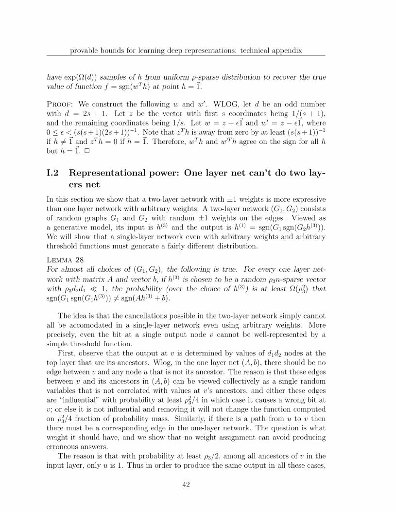
provable bounds for learning deep representations: technical appendix
have exp(Ω(d)) samples of h from uniform ρ-sparse distribution to recover the truevalue of function f = sgn(wTh) at point h = ~1.
Proof: We construct the following w and w′. WLOG, let d be an odd numberwith d = 2s + 1. Let z be the vector with first s coordinates being 1/(s + 1),and the remaining coordinates being 1/s. Let w = z + ε~1 and w′ = z − ε~1, where0 ≤ ε < (s(s+ 1)(2s+ 1))−1. Note that zTh is away from zero by at least (s(s+ 1))−1
if h 6= ~1 and zTh = 0 if h = ~1. Therefore, wTh and w′Th agree on the sign for all hbut h = ~1. 2
I.2 Representational power: One layer net can’t do two lay-ers net
In this section we show that a two-layer network with ±1 weights is more expressivethan one layer network with arbitrary weights. A two-layer network (G1, G2) consistsof random graphs G1 and G2 with random ±1 weights on the edges. Viewed asa generative model, its input is h(3) and the output is h(1) = sgn(G1 sgn(G2h
(3))).We will show that a single-layer network even with arbitrary weights and arbitrarythreshold functions must generate a fairly different distribution.
Lemma 28For almost all choices of (G1, G2), the following is true. For every one layer net-
work with matrix A and vector b, if h(3) is chosen to be a random ρ3n-sparse vectorwith ρ3d2d1 1, the probability (over the choice of h(3)) is at least Ω(ρ2
3) thatsgn(G1 sgn(G1h
(3))) 6= sgn(Ah(3) + b).
The idea is that the cancellations possible in the two-layer network simply cannotall be accomodated in a single-layer network even using arbitrary weights. Moreprecisely, even the bit at a single output node v cannot be well-represented by asimple threshold function.
First, observe that the output at v is determined by values of d1d2 nodes at thetop layer that are its ancestors. Wlog, in the one layer net (A, b), there should be noedge between v and any node u that is not its ancestor. The reason is that these edgesbetween v and its ancestors in (A, b) can be viewed collectively as a single randomvariables that is not correlated with values at v’s ancestors, and either these edgesare “influential” with probability at least ρ2
3/4 in which case it causes a wrong bit atv; or else it is not influential and removing it will not change the function computedon ρ2
3/4 fraction of probability mass. Similarly, if there is a path from u to v thenthere must be a corresponding edge in the one-layer network. The question is whatweight it should have, and we show that no weight assignment can avoid producingerroneous answers.
The reason is that with probability at least ρ3/2, among all ancestors of v in theinput layer, only u is 1. Thus in order to produce the same output in all these cases,
42
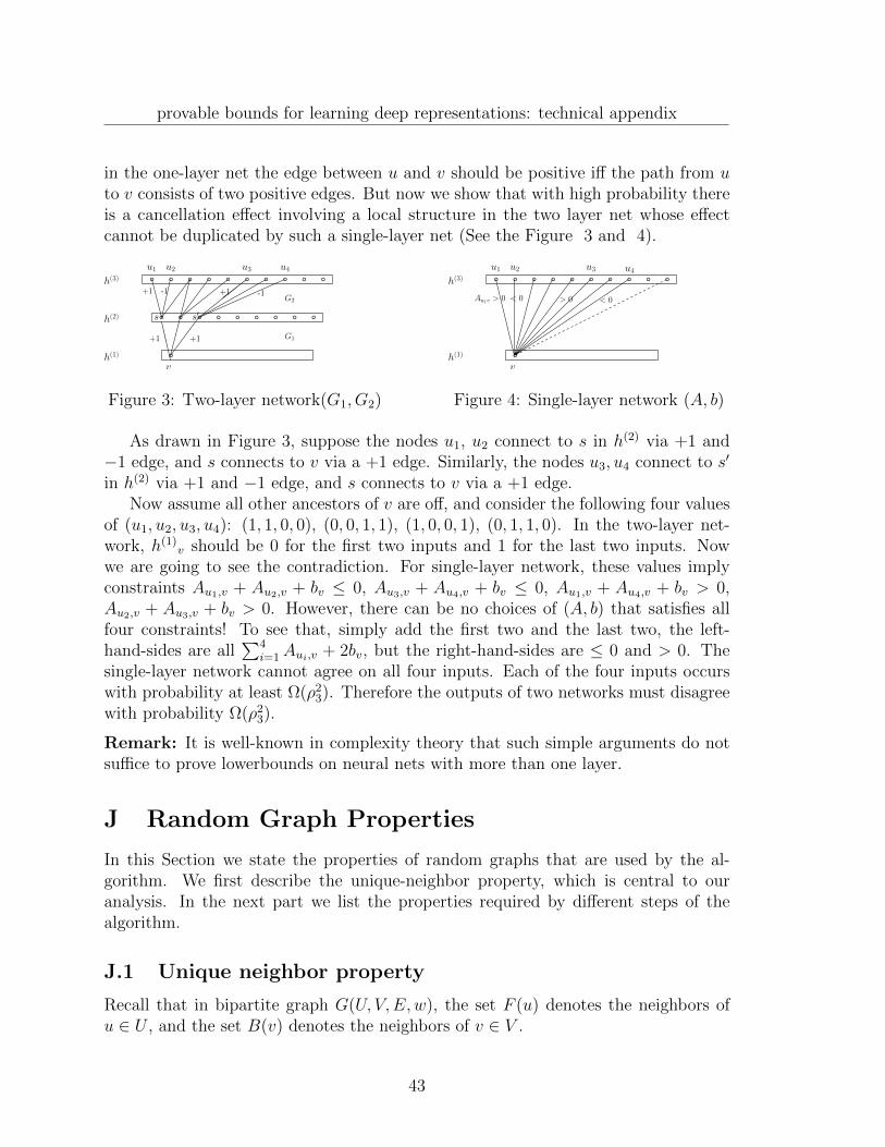
provable bounds for learning deep representations: technical appendix
in the one-layer net the edge between u and v should be positive iff the path from uto v consists of two positive edges. But now we show that with high probability thereis a cancellation effect involving a local structure in the two layer net whose effectcannot be duplicated by such a single-layer net (See the Figure 3 and 4).
h(1)
h(2)
v
+1 -1
+1
u1 u2 u3h(3)
+1
+1
G2
G1
s s′
u4
-1
Figure 3: Two-layer network(G1, G2)
h(1)
v
u1 u2 u3h(3)
Au1v > 0 < 0 > 0
u4
< 0
Figure 4: Single-layer network (A, b)
As drawn in Figure 3, suppose the nodes u1, u2 connect to s in h(2) via +1 and−1 edge, and s connects to v via a +1 edge. Similarly, the nodes u3, u4 connect to s′
in h(2) via +1 and −1 edge, and s connects to v via a +1 edge.Now assume all other ancestors of v are off, and consider the following four values
of (u1, u2, u3, u4): (1, 1, 0, 0), (0, 0, 1, 1), (1, 0, 0, 1), (0, 1, 1, 0). In the two-layer net-work, h(1)
v should be 0 for the first two inputs and 1 for the last two inputs. Nowwe are going to see the contradiction. For single-layer network, these values implyconstraints Au1,v + Au2,v + bv ≤ 0, Au3,v + Au4,v + bv ≤ 0, Au1,v + Au4,v + bv > 0,Au2,v + Au3,v + bv > 0. However, there can be no choices of (A, b) that satisfies allfour constraints! To see that, simply add the first two and the last two, the left-hand-sides are all
∑4i=1Aui,v + 2bv, but the right-hand-sides are ≤ 0 and > 0. The
single-layer network cannot agree on all four inputs. Each of the four inputs occurswith probability at least Ω(ρ2
3). Therefore the outputs of two networks must disagreewith probability Ω(ρ2
3).
Remark: It is well-known in complexity theory that such simple arguments do notsuffice to prove lowerbounds on neural nets with more than one layer.
J Random Graph Properties
In this Section we state the properties of random graphs that are used by the al-gorithm. We first describe the unique-neighbor property, which is central to ouranalysis. In the next part we list the properties required by different steps of thealgorithm.
J.1 Unique neighbor property
Recall that in bipartite graph G(U, V,E,w), the set F (u) denotes the neighbors ofu ∈ U , and the set B(v) denotes the neighbors of v ∈ V .
43
provable bounds for learning deep representations: technical appendix
For any node u ∈ U and any subset S ⊂ U , let UF (u, S) be the sets of uniqueneighbors of u with respect to S,
UF (u, S) , v ∈ V : v ∈ F (u), v 6∈ F (S \ u)
Property 1 In a bipartite graph G(U, V,E,w), a node u ∈ U has (1 − ε)-uniqueneighbor property with respect to S if
∑
v∈UF (u,S)
|w(u, v)| ≥ (1− ε)∑
v∈F (u)
|w(u, v)| (2)
The set S has (1 − ε)-strong unique neighbor property if for every u ∈ U , u has(1− ε)-unique neighbor property with respect to S.
Remark 4 Notice that in our definition, u does not need to be inside S. This is notmuch stronger than the usual definition where u has to be in S: if u is not in S weare simply saying u has unique neighbor property with respect to S ∪ u. Whenall (or most) sets of size |S|+ 1 have the “usual” unique neighbor properties, all (ormost) sets of size |S| have the unique neighbor property according to our definition.
Lemma 29If G(U, V,E) is from distribution Gm,n,p, and for any u ∈ U , the weight vector w(u, ·)(i.i.d. on edges) satisfies that |w(u, ·)|21 ≥ C · ‖w(u, ·)‖2
2 for some C. Then for everysubset S of U with (1 − p)|S| > 1 − ε/2 (note that p|S| = d′|S|/n is the expecteddensity of F (S)), with probability 1 − 2m exp(−ε2C) over the randomness of thegraph, S has the (1− ε)-strong unique neighbor property.
Note: The weights usually comes from one of the following: 1. all weights are 1;2. weights are random in ±1; 3. weights are random in [−1, 1]. In all these casesC is Θ(d′).Proof:
Fix the vertex u, first sample the edges incident to u. Without loss of generalityassume u has neighbors v1, . . . , vk (where k ≈ pn). Now sample the edges incident tothe vi’s. For each vi, with probability (1− p)|S| ≥ 1− ε/2, vi is a unique neighbor ofu. Call this event Goodi (and we also use Goodi as the indicator for this event).
By the construction of the graph we know Goodi’s are independent, hence byHoeffding inequality (see Theorem 45), we have that with probability
1−2 exp(−ε2(∑
v∈F (u) w(u, v))2
∑v∈F (u) w(u, v)2
) = 1−2 exp(−ε2|w(u, ·)|21/‖w(u, ·)‖22) = 1−2 exp(−ε2C),
the following holds∑
v∈F (u)
w(u, v)Goodi ≥ (1− ε)∑
v∈F (u)
w(u, v).
44
provable bounds for learning deep representations: technical appendix
By union bound, every u satisfies this property with probability at least 1 −2m exp(−ε2C). 2
Corollary 30IfG(U, V,E) is chosen from Gm,n,p and all the weights w(u, v) have the same magnitudefor (u, v) ∈ E , then for fixed S with p|S| < ε/2, with probability 1− exp(−Ω(d′)), Shas the (1− ε)-strong unique neighbor property.
J.2 Properties required by each steps
We now list the properties required in our analysis. These properties hold with highprobability for random graphs.
J.2.1 Single layer
The algorithm PairwisGraph requires the following properties Psing
1. For any u in the observed layer, |B(u)| ∈ [0.9d, 1.1d], (if G has negative weights,we also need |B+(u)| ∈ [0.9d/2, 1.1d/2])
2. For any z in the hidden layer, |F (z)| ∈ [0.9d′, 1.1d′], (if G has negative weights,we also need |F+(z)| ∈ [0.45d′, 0.55d′])
The algorithm 3-WiseGraph needs Psing, and additionally Psing+1. For any u, v in the observed layer, |B+(u) ∪B+(v)| ≤ 10.
Lemma 31If graph G is chosen from Gm,n,p with expected degrees d, d′ log n, with high
probability over the choice of the graph, Psing is satisfied. If in addition d2 ≤ n4/5,the property Psing+ is also satisfied with high probability.
J.2.2 Multi-layer
For the multi-layer setting, the algorithm PairwisGraph requires the following expan-sion properties Pmul.
1. For any node u at the layer i, |Fi−1(u)| ∈ [0.9d′i−1, 1.1d′i−1], |Bi(u)| ∈ [0.9di, 1.1di],∣∣F+
i−1(u)∣∣ ∈ [0.45d′i−1, 0.55d′i−1],
∣∣B+i (u)
∣∣ ∈ [0.45di, 0.55di]
2. For any node u at the layer i, |B(t)+ (u)| ≥ 0.8ρi/ρt, and |B(`)(u)| ≤ 2`−i+1ρi/ρ`.
3. For any pair of nodes u, v at layer i,
∣∣∣B(`)+ (u) ∩B(`)
+ (v)∣∣∣ ≤ 2ρi+1/ρ` ·
(log n/di+1 + 1/(ρ`n`) +
∣∣∣B(i+1)+ (u) ∩B(i+1)
+ (v)∣∣∣)
45
provable bounds for learning deep representations: technical appendix
In particular, if u and v have no common positive parent at layer i+1 (∣∣∣B(i+1)
+ (u) ∩B(i+1)+ (v)
∣∣∣ =
0), then ∣∣∣B(`)+ (u) ∩B(`)
+ (v)∣∣∣ ≤ o(ρi+1/ρ`)
The algorithm 3-WiseGraph needs property Pmul+:
1. Properties 1 and 2 in Pmul
2. For any pair of nodes u, v at layer i,∣∣∣B(`)
+ (u) ∩B(`)+ (v)
∣∣∣ ≤ 10ρi+1/ρ`
3. For any three nodes u, v and s at layer i, if they don’t have a common positiveneighbor in layer i+ 1,
∣∣∣B(`)+ (u) ∩B(`)
+ (v) ∩B(`)+ (s)
∣∣∣≤ 2ρi+1/ρ` ·
(log n/di+1 + ρ`/(ρ`n`) + 1/(ρ2
`n2`))≤ o(ρi+1/ρ`)
Lemma 32If the network D(`, ρ`, Gi) have parameters satisfying di log n, and ρ2
i ρi+1,then with high probability over the randomness of the graphs, Gi’s satisfy Pmul.Additionally, if di log n and ρ3
i ρi+1, then Gi’s satisfy Pmul+ with highprobability.
In order to prove Lemma 32 we need the following claim:
Claim 33If the graph G ∼ Gm,n,p with d = pm being the expected back degree, and d log n.For two arbitrary sets T1 and T2, with d|T1| m, d|T2| m, we have with highprobability
|B(T1) ∩B(T2)| ≤ (1 + ε)d|T1 ∩ T2|+ (1 + ε)d2|T1||T2|/m+ 5 log n
This Claim simply follows from simple concentration bounds. Now we are readyto prove Lemma 32.Proof:[Proof of Lemma 32] Property 1 in Pmul follows directly from di log n.
Property 2 in Pmul follows from unique neighbor properties (when we view thebipartite graph from Ni to Ni+1).
For Property 3, we prove the following proposition by induction on t:
Proposition 34For any two nodes u, v at layer 1,
∣∣∣B(t)+ (u) ∩B(t)
+ (v)∣∣∣ ≤ (1+ε)ttρ2
1/(ρ2tnt)+6t(1+ε)tρ3 log n/ρt+(1+ε)tρ2
∣∣∣B(2)+ (u) ∩B(2)(v)
∣∣∣ /ρt
46
provable bounds for learning deep representations: technical appendix
This is true for t = 2 (by Claim 33). Suppose it is true for all the values less thant − 1. By Claim 33, we know with high probability (notice that we only need to dounion bound on n2 pairs)
∣∣∣B(t+1)+ (u) ∩B(t+1)
+ (v)∣∣∣ ≤ (1 + ε)dt/2 · ρ2
∣∣∣B(t)+ (u) ∩B(t)
+ (v)∣∣∣ /ρt
+(1 + ε)d2t/4 · |B(t)
+ (u)||B(t)+ (v)|+ 5 log n
≤ (1 + ε)t+1ρ2
∣∣∣B(2)+ (u) ∩B(2)(v)
∣∣∣ /ρt+1 + 6t(1 + ε)t+1ρ3 log n/ρt+1
+(1 + ε)ttρ21/(ρ
2tnt) + (1 + ε)d2
t/4 · ρ21/(ρ
2tnt+1) + 5 log
≤ (1 + ε)t+1ρ2
∣∣∣B(2)+ (u) ∩B(2)(v)
∣∣∣ /ρt+1 + 6(t+ 1)(1 + ε)t+1ρ3 log n/ρt+1
+2(1 + ε)t+1(t+ 1)ρ21/(ρ
2t+1nt+1),
where the last inequality uses the fact that ρ21/(ρ
2tnt) ≤ d2
t/4 · ρ21/(ρ
2tnt+1). This is
because ntdt/nt+1 = d′t 1.Proposition 34 implies that when ρ2
1 ρ2, and ` is a constant,
∣∣∣B(t)+ (u) ∩B(t)
+ (v)∣∣∣ ≤ 2ρi+1/ρ` ·
(1/di+1 + 1/(ρ`n`) +
∣∣∣B(i+1)+ (u) ∩B(i+1)
+ (v)∣∣∣)
Property 3 in Pmul+ is similar but more complicated. 2
J.2.3 Properties for Graph Reovery
For the algorithm RecoverGraph3Wise to work, the hypergraph generated from therandom graph should have the following properties Precovery+.
1’ For any (v1, v2, v3) ∈ E, if S is the set defined as in the algorithm, then|S\F (B(v1) ∩B(v2) ∩B(v3))| < d′/20.
2’ For any u1, u2 ∈ U , |F (u1) ∪ F (u2)| > 1.5d′.
3’ For any u ∈ U , v ∈ V and v 6∈ F (u), v is correlated with at most d′2/40 pairsin F (u).
4’ For any u ∈ U , at least 0.1 fraction of triples v1, v2, v3 ∈ F (u) does not have acommon neighbor other than u.
5’ For any u ∈ U , its degree is in [0.8d′, 1.2d′]
J.2.4 Properties for Partial Encoder
For the Partial Encoder algorithm to work, we only need the support of h satisfyingthe strong unique-neighbor property.
47
provable bounds for learning deep representations: technical appendix
J.2.5 Properties for Learning the graph
In order to learn the −1 weights, the conditions we need are similar to Pmul andPmul+.
In the case with real weights, we don’t need any assumptions on the graph, becausewe are relying on VC-dimension arguments.
K Auxiliary Lemmas for uniform ρ`n` sparse vec-
tors
In this subsection, we provide lemmas about the uniform ρn-sparse vector of dimen-sion n.
These Lemmas suggest that when looking at intersections with relatively smallsets, uniform ρn sparse vector behaves like i.i.d. Bernoulli variables with probabilityρ. Also, in this section the sparse vector is identified by its support S.
Lemma 35If S is a uniformly random ρn-sparse subset of [n], then for any fix set T with ρ|T | 1and |T | n,
1− ρ|T |/2 ≥ Pr[T ∩ S = ∅] ≥ 1− ρ|T |
Proof: For each t ∈ T , Pr[t ∈ S] = ρ. By union bound, Pr[T ∩ S = ∅] ≥1−∑t∈S Pr[t ∈ S] = 1− ρ|T |.
On the other hand, let ρn = k, we have,
Pr[T ∩ S = ∅] = (1− k
n) · (1− k
n− 1) . . . (1− k
n− |T |) ≤ (1− k
n)|T | ≤ 1− ρ|T |/2
2
Lemma 36If S is a uniformly random ρn-sparse subset of [n], then for any fix set T with ρ|T | 1and |T | n, ρ|T | ≥ Pr[|S ∩ T | = 1] ≥ ρ|T |/2
Proof: For any t ∈ T , we compute Pr[S ∩ T = t]. Conditioned on t ∈ T , S \ tis uniform (ρn− 1)-sparse subset of [n] \ t, thus by the Lemma above,
Pr[S ∩ T = t] = Pr[t ∈ S] · Pr[S ∩ (T \ t) = ∅] ∈ [ρ/2, ρ]
All the events S ∩ T = t for t ∈ T are disjoint, thus ρ|T | ≥ Pr[|S ∩ T | = 1] ≥ρ|T |/2 2
Lemma 37If S is uniform random ρn-sparse subset of [n], then for any fix set T with ρ|T | 1and |T | n,
Pr[|T ∩ S| > ρn/2] < (2ρ|T |)ρn/2
48
provable bounds for learning deep representations: technical appendix
Proof: Let k = ρn. For any subsets M of T of size k, Pr[M ⊂ S] = kn·
kn−1
. . . kn−(k/2)
≤ (2ρ)k/2. Taking a union bound over all M , we have Pr[|T ∩ S| ≥k/2] ≤
( |T |k/2
)(2ρ)k/2 ≤ (2ρ|T |)k/2. 2
Lemma 38If S is a uniformly random ρn-sparse set, then for any two disjoint sets T1 and T2
with ρ|T1| 1, ρ|T2| 1 and |T1|, |T2| n,
ρ2|T1||T2|/5 ≤ Pr[S ∩ T1 6= ∅, S ∩ T2 6= ∅] ≤ 2ρ2|T1||T2|Proof: From Lemma 36 we know Pr[|S ∩ T1| = 1] ∈ [ρ|T1|/2, ρ|T1|].Conditioned on|S ∩ T1| = 1, S \ T1 is a random ρn − 1 sparse vector in n − |T1| dimension. ApplyLemma 36 with ρ′ = (ρn − 1)/(n − |T1|) we have Pr[|S ∩ T2| = 1 | |S ∩ T1| = 1] =Θ(ρ′|T2|).
On the other hand, ρ|T1| is an upperbound on Pr[S ∩ T1 6= ∅], ρ′|T2| is an upper-bound on Pr[S ∩ T2 6= ∅|S ∩ T1 6= ∅], so we get the other direction. 2
Lemma 39If S is a uniformly random ρn-sparse subset of [n], then for two disjoint sets T1, T2
with ρ|T1|, ρ|T2| 1 and |T1|, |T2| n,
ρ|T1|/2 ≤ Pr[S ∩ T1 6= ∅, S ∩ T2 = ∅] ≤ 2ρ|T1|
The proof is very similar to Lemma 38.
Lemma 40If S is a uniform random ρn-sparse subset of [n], then for any three sets T1, T2 and T3
with ρ|T1|, ρ|T2|, ρ|T3| 1 and |T1|, |T2|, |T3| n. Let max|Ti| ≤ A,max1≤i<j≤3 |Ti∩Tj| = B, and |T1 ∩ T2 ∩ T3| = C, then
Pr[(S ∩ Ti 6= ∅) for i = 1, 2, 3] ≤ O(ρ3A3 + ρ2AB + ρC)
Proof: The proof is not hard but tedious. It enumerates all the possible ways Scan intersect with all three Ti’s.
Let K1 = T1 − T2 ∪ T3, K2 = T2 − T1 ∪ T3, K3 = T3 − T1 ∪ T2. Also, letK12 = T1 ∩ T2 − T3 (similarly define K23, K31). Finally let K123 = T1 ∩ T2 ∩ T3.
Let E be the event that S ∩ K1 6= ∅, S ∩ K2 6= ∅, S ∩ K3 6= ∅; E ′ be the eventthat S ∩K123 6= ∅; E12 be the event that S ∩K12 6= ∅, S ∩K3 6= ∅ (similarly defineE23 and E31). The event S ∩ Ti 6= ∅ for all i = 1, 2, 3 is contained in the union ofthese events E ∪ E ′ ∪ E12 ∪ E23 ∪ E31. By previous Lemmas it is easy to boundPr[E] ≤ 2ρ3|T1||T2||T3| ≤ 2ρ3A3, Pr[E ′] ≤ ρC, and Pr[E12] ≤ 2ρ2|K12||K3| ≤ 2ρ2AB.Hence Pr[(S ∩ Ti 6= ∅) for i = 1, 2, 3] ≤ O(ρ3A3 + ρ2AB + ρC) 2
L Omitted Proofs in Section H
In this Section we shall prove Theorem 24 and Theorem 25.
49
provable bounds for learning deep representations: technical appendix
Proving Theorem 24 By the structure of the network we know
E[yuyvys] =∑
i∈B(u),j∈B(v),k∈B(s)
wi,uwj,vwk,s E[hihjhk] (3)
Observe that wi,u and wj,v are different random variables, no matter whether i is equalto j. Thus by 3-order Hoeffding inequality stated in Lemma 47, with high probabilityover the choice of the weights
|E[yuyvys]| ≤√ ∑
i∈B(u),j∈B(v),k∈B(s)
E[hihjhk]2 log3 n (4)
Let V be the main term in the bound:
V ,∑
i∈B(u),j∈B(v),k∈B(s)
E[hihjhk]2.
Define Buv = B(u) ∩ B(v), Bvs = B(v) ∩ B(s), Bsu = B(s) ∩ B(u). Similar toProperty Psing+, for a random graph we know all these sets have size at most 10.
The following claim gives bound on the variance term (so we know E[yuyvys] hassmall absolute value when they don’t share a common neighbor):
Claim 41If h is uniform random ρm-sparse vector, and B(u)∩B(v)∩B(s) = ∅, and |Buv| ≤ 10,|Bvs| ≤ 10 and |Bsu| ≤ 10, then
V =∑
i∈B(u),j∈B(v),k∈B(s)
E[hihjhk]2 ≤ O(ρ6d3 + ρ4d)
Proof:First of all, for any triple (i, j, k) such that i, j, k are distinct, the expectation
E[hihjhk] ≤ ρ3. The total number of such triples is at most O(d3). The contributionto the sum V is O(d3ρ6)
Then we count the triples (i, j, k) with i = j, and i 6= k (i ∈ Buv and k ∈ B(s)).The total number of such triples (i, j, k) is bounded by 10d. In this case, E[hihjhk] ≤ρ2. Thus the total contribution to the V is O(dρ4). The other two symmetric caseshave similar contribution to the V as well.
Hence the total sum is bounded by O(ρ6d3 + ρ4d). 2
When u, v, s share a common neighbor, the following claim shows E[yuyvys] has alarge absolute value.
Claim 42If h is uniform random ρm-sparse vector , and B(u) ∩ B(v) ∩ B(s) = z, and|Buv| ≤ 10, |Bvs| ≤ 10 and |Bsu| ≤ 10, then with high probability over the choice ofthe weights
|E[yuyvys]| ≥ ρ−O(
√(ρ6d3 + ρ4d) log3 n)
50
provable bounds for learning deep representations: technical appendix
Proof: Let Az,z,z = 0, and Ai,j,k = E[hihjhk] when (i, j, k) 6= (z, z, z). Thus
E[yuyvys] =∑
i∈B(u),j∈B(v),k∈B(s)
wi,uwj,vwk,s E[hihjhk]
= wz,uwz,vwz,s E[hz] +∑
i∈B(u),j∈B(v),k∈B(s)
wi,uwj,vwk,sAi,j,k (5)
Similar to the previous case, we know that∑
i∈B(u),j∈B(v),k∈B(s)
A2i,j,k ≤ O(ρ6d3 + ρ4d)
and thus with high probability,
|∑
i∈B(u),j∈B(v),k∈B(s)
wi,uwj,vwk,sAi,j,k| ≤√ ∑
i∈B(u),j∈B(v),k∈B(s)
A2i,j,k log3 n
≤ O(
√(ρ6d3 + ρ4d) log3 n)
By Equation (5), the expectation can be bounded by
E[yuyvys] = wz,uwz,vwz,s E[hz]±O(
√(ρ6d3 + ρ4d) log3 n),
which implies
|E[yuyvys]| ≥ ρ−O(
√(ρ6d3 + ρ4d) log3 n)
2
The Theorem follows directly from these two claims.
Extending Theorem 24 to distribution D1 Using similar ideas, and the boundsfrom Section E, we can prove Theorem 25.
We shall first extend Theorem 25 to the setting when h is generated by the upperlevels of the network (call the distribution D1). In order to do this we need to bound
E[hihjhk] carefully. Following similar ideas as Lemma 12, we have
Proposition 43If h ∼ D1, then
E[hihjhk] is
≤ O(ρ3
1 + ρ2ρ1 + ρ2) if B+(i) ∩B+(j) ∩B+(k) 6= ∅,≤ O(ρ3
1 + ρ2ρ1 + ρ3) if B+(i) ∩B+(j) ∩B+(k) = ∅,
and
E[hihj] is
≤ O(ρ2
1 + ρ2) if B+(i) ∩B+(j) 6= ∅,≤ O(ρ2
1 + ρ3) if B+(i) ∩B+(j) = ∅,
51
provable bounds for learning deep representations: technical appendix
Basically, most pairs/triples still have small expectation. The following Proposi-tion shows there are only a very small number of pairs that are highly correlated.
Proposition 44For a fixed set T of size at most 3d in layer 1, when d5
1 < n, with high probability,the number of pairs i, j ∈ T, i 6= j such that B+(i) ∩B+(j) 6= ∅ is at most 10.
Proof: For any node q in layer 2, let Cq =∣∣(i, j) : i, j ∈ T, (q, i), (q, j) ∈ E+
1
∣∣. Byrandomness of the graph we know E[Cq] ≤ d4/n2. Summing over all nodes in layer2, we have E[
∑q Cq] ≤ d4/n ≤ n−0.2. With high probability,
∑q Cq ≤ 10. (Note that
Cq are independent variables.) 2
With Proposition 43 and 44, we are ready to extend Theorem 24 to the moregeneral distribution.
As before we need to bound the variance. When B(u) ∩ B(v) ∩ B(s) = ∅, webound the variance V =
∑i∈B(u),j∈B(v),k∈B(s) E[hihjhk]
2 as follows:
First of all, there are at most O(d3) triples of (i, j, k) such that i, j, k are distinct.Typically, each one contribute to V with E[hihjhk] ≤ O((ρ3
1 + ρ2ρ1 + ρ3)2). However,there might be at most 10 triples with higher expectation (by Proposition 44), so thefinal bound is O((ρ3
1 + ρ2ρ1 + ρ2)2). The total contribution of these triples is
v1 = O(d3(ρ31 + ρ2ρ1 + ρ3)2) +O((ρ3
1 + ρ2ρ1 + ρ2)2)
There are at most 10d triples of (i, j, k) such that i = j ∈ Buv and i 6= k. Thecontribution of these triples is at most ρ2
1 +ρ2. Thus the total contribution is at most
v2 ≤ 10d(ρ21 + ρ2)2).
Combining all these we know√V ≤ √v1 + v2 ≤ d3/2(ρ3
1 +ρ2ρ1 +ρ3)+(ρ31 +ρ2ρ1 +
ρ2) + 10d1/2(ρ21 + ρ2).
Under the assumption of Theorem 25,√V log3 n ≤ ρ1/3. With high probabil-
ity, when u, v, s do not share a common neighbor, we know |E[yuyvys]| ≤ ρ1/3 ;when u, v, s share a unique neighbor z, we know |E[yuyvys]| ≥ 2ρ1/3. Therefore thealgorithm can distinguish them.
Modifications in Graph Recovery If edge weights are ±1, the same algorithmworks because with high probability there are no more than a constant number oftriples u, v, s in the observed layer that share more than 1 neighbor (this is impliedby Proposition 43).
When edge weights are in [−1, 1], the hypergraph only satisfy the following ap-proximate conditions: if u, v, s share a common parent z and the edges from z tou, v, s all have weight outside [−0.01, 0.01], (u, v, s) is an edge in the hypergraph; ifu, v, s do not share a common parent, then (u, v, s) is not an edge. All other casesare ambiguous. Graph Recovery in this case can again be done by the same algo-rithm, because there are only a small constant fraction of ambiguous edges, and thethresholds in the algorithm tolerates a small constant fraction of error.
52
provable bounds for learning deep representations: technical appendix
Modifications in PartialEncoder Note that in this case graph recovery gives alledges, instead of positive edges, so we cannot directly use those for PartialEncoder.However, the expectation E[yuyvys] is positive and large, even if they share a commonparent z and there are even number of positive edges from z to u, v, s. Using thisinformation it is easy to separate the positive and negative edges, see Algorithm 9.
Algorithm 9. LearnLastLayer
Input: E, the set of edgesOutput: E+, E−, the set of positive and negative edges
for each node x ∈ h(1) doPick u, v in F (x)Let S be the set s : Eh[yuyvys] > 0.for each t : (x, t) ∈ E do
if most triples (t, u′, v′)(u′, v′ ∈ S) have positive Eh[ytyu′yv′ ] thenadd (x, t) to E+
elseadd (x, t) to E−
end ifend for
end for
When weights are +1,−1 we are already done.When the weights are in [−1, 1] we don’t find all the positive edges (1% of the
edges are missing because they have small weights), but this is again OK because thePartialEncoder can tolerate small constant fraction of error.
Modifications in Learning Decoder For learning decoder, since we do not havethresholds at the last layer, we only need to solve a system of linear equations.
M Standard Concentration Bounds
We use the following version of Hoeffding’s inequality.
Theorem 45[Hoe63] X1, . . . , Xn are independent random variables such that Xi ∈ [ai, bi] almostsurely. Let S = X1 + · · ·+Xn. Then
Pr[|S − E[S]| ≥ t] ≤ 2 exp(−2t2∑n
i=1(ai − bi)2)
Using this (and with union bound) it is easy to prove the following bilinear andtrilinear bounds (these are not tight but we don’t mind losing log n factors).
53
provable bounds for learning deep representations: technical appendix
Lemma 46If w, w′ are independent random vectors in −1, 1d, then with high probability
|∑
i,j
wiw′jAi,j| ≤ O
√∑
i,j
A2i,j log2 n
Proof: We are going to bound xTAy, which is equal to
xTAy =d∑
i=1
xi
(∑
j
Ai,jyj
)
With high probability over the choice of y, for any i,∑
j Ai,jyj ≤ O(√∑
j Ai,j2 log n).
When these events happen, we have that
xTAy =d∑
i=1
xi
(∑
j
Ai,jyj
)≤∑
i
xiO(
√∑
j
Ai,j2 log n).
By Hoeffding inequality again, we have that with high probability over the choiceof x,
xTAy ≤∑
i
xiO
√∑
j
Ai,j2 log n
≤ O
√∑
i,j
Ai,j2 log2 n
2
Lemma 47If w, w′, w′′ are independent random vectors in −1, 1d, then with high probability
|∑
i,j,k
wiw′jw′′kAi,j,k| ≤ O
√∑
i,j,k
A2i,j,k log3 n
The proof is very similar to Lemma 46.
54