PROPERTIES OF MINIMIZERS OF AVERAGE-DISTANCE … · properties of minimizers of average-distance...

PROPERTIES OF MINIMIZERS OF AVERAGE-DISTANCE PROBLEM VIADISCRETE APPROXIMATION OF MEASURES

XIN YANG LU AND DEJAN SLEPCEV

ABSTRACT. Given a finite measure µ with compact support, and λ > 0, the average-distance problem, in the penalized formulation, is to minimize

(0.1) Eλµ(Σ) :=

∫Rd

d(x,Σ)dµ(x) + λH1(Σ),

among pathwise connected, closed sets, Σ. Here d(x,Σ) is the distance from a pointto a set and H1 is the 1-Hausdorff measure. In a sense the problem is to find a one-dimensional measure that best approximates µ. It is known that the minimizer Σ is topo-logically a tree whose branches are rectifiable curves. The branches may not be C1, evenfor measures µ with smooth density. Here we show a result on weak second-order reg-ularity of branches. Namely we show that arc-length-parameterized branches have BVderivatives and provide a priori estimates on the BV norm.

The technique we use is to approximate the measure µ, in the weak-∗ topology of mea-sures, by discrete measures. Such approximation is also relevant for numerical compu-tations. We prove the stability of the minimizers in appropriate spaces and also comparethe topologies of the minimizers corresponding to the approximations with the mini-mizer corresponding to µ.

Keywords. nonlocal variational problem, average-distance problem, regularityClassification. 49Q20, 49K10, 49Q10, 35B65

1. INTRODUCTION

The average-distance problem was introduced by Buttazzo, Oudet and Stepanov in[1]. In the penalized formulation the problem takes the form

Problem 1.1. For d ≥ 2, given a finite compactly supported measure µ, and λ > 0, minimize

(1.1) Eλµ(Σ) =

∫Rd

d(x,Σ)dµ(x) + λH1(Σ)

among pathwise connected, closed sets Σ.

We define the set of admissible candidates by

A := {Σ ⊆ Rd : Σ compact, pathwise connected, andH1(Σ) <∞}.

Date: January 8, 2013.1

2 XIN YANG LU AND DEJAN SLEPCEV

For the future reference we denote the part of the energy functional which measures theapproximation error by

Fµ(Σ) :=

∫Rd

d(x,Σ)dµ.

This problem has many applications: a simple one is• µ is the distribution of passengers,• Σ is a transport network.

In this case Fµ(Σ) is the average distance of passengers from the network, and H1(Σ)is the cost to build such network. Minimizing Eλ

µ is determining the network with bestserves the passengers, under cost considerations.

An alternative interpretation is found in cloud data systems:• µ is the distribution of data points,• Σ is a one dimension object which approximates the data.

In this case Fµ(Σ) is the approximation error, while λH1(Σ) is the cost associated to thecomplexity of such representation. Minimizing Eλ

µ is determining the best approxima-tion, accounting for the complexity.

Existence of minimizers, follows from theorems of Blaschke and Gołab, [1]. Geomet-ric properties of minimizers were investigated by Buttazzo, Oudet and Stepanov [1],Buttazzo and Stepanov [2, 3] (mainly in two dimensions) and by Paolini and Stepanov[9] (for higher dimensions). Let us also add that Lemenant [6] provides an excellent re-view of the current knowledge about average-distance problem. It has been proven thatminimizers are topologically trees with rectifiable branches. Furthermore no more thanthree branches can meet at a point. Regarding the regularity of branches the followingresults are available:

• In [1] it has been proven that minimizers are Ahlfors regular in two dimensionaldomains. The result was extended to higher dimensional domains in [9],• In [2] it has been proven that minimizers are union of Lipschitz curves; for the

penalized problem, it is easy to prove that this union if finite (e.g. using Theorem3.4).• In [12] it has been proven that regularity beyond C1,1 cannot be expected in the

general case.• In [10] an explicit counterexample to C1 regularity for minimizers has been con-

structed.We recall that in two dimensional domains, in the constrained formulation

minH1(Σ)≤L

Fµ(Σ),

in [11] it has been proven that given a minimizer Σ, (which is finite union of Lipschitzcurves {γi}Ni=1, as proven in [2]), if (part of) γj satisfies a geometric condition then it is

PROPERTIES OF MINIMIZERS OF AVERAGE-DISTANCE PROBLEM 3

is C1,1. Moreover, in [7] which studies the average-distance problem in two dimensionsprovides "tilt estimates" which are related to our regularity estimates.

This paper aims to extend such regularity results, and prove that minimizers are finiteunions of Lipschitz curves with BV derivatives. More precisely we show that given anarbitrary nonnegative finite measure with compact support, µ, and λ > 0, any solutionΣ ∈ argmin Eλ

µ is finite union of Lipschitz curves {γk}Nk=1 (without loss of generalityassume that all γk are arc-length parameterized), such that for any k = 1, . . . , N it holds

(1.2)∑k

‖γ′k‖TV ≤1

λ|µ(Rd)|,

where ‖ · ‖TV denotes the total variation.In other words we provide an estimate on the total curvature of the curves that make

up Σ, where the curvature, κ = γ′′k is understood as the signed measure. The fact the thetotal mass (times 1/λ) bounds the curvature is not surprising. To motivate it let us as-sume that the minimizer Σ is a single smooth curve and that µ is absolutely continuouswith respect to Lebesgue measure. Let Π be the projection onto Σ (it is known that Πhas unique value almost everywhere). Then the first variation for the Problem 1.1 givesthat for any smooth vector field v : Σ→ Rd supported away from the endpoints of Σ

−∫

Σ

κ · vdH1(Σ) =1

λ

∫Rd

(x− Π(x))

|x− Π(x)|· v((Π(x))dµ(x).

Taking supremum over all v, as above, with |v| ≤ 1 implies (1.2).The difficulties one faces in applying the reasoning above are that Σ is neither regular

nor a curve and that µ is not assumed to be absolutely continuous with respect to theLebesgue measure.

The approach used is based on approximating a measure µ by a sequence discretemeasures {µn}

∗⇀µ, and analyzing the minimizers of Problem 1.1 with µ replaced by µn.

In addition to the estimate on the BV norm we prove a topological relation betweenminimizers of Eλ

µn and minimizers of Eλµ , with λ > 0 arbitrarily given.

This paper is structured as follows:• In Section 2 we recall the known results on the average-distance problem, intro-

duce the discrete approximations and prove a couple of preliminary results.• In Section 3 we prove an upper bound on the number endpoints of minimizers

and analyze the behavior of endpoints in the approximation process. In particu-lar we prove in Theorem 3.4 that if µn are discrete approximations of µ and Σn areminimizers of Eλ

µn which converge to Σ, a minimizer of Eλµ , then each endpoint

of Σ is a limit of endpoints of Σn.• Section 4 is devoted to the topological comparison between minimizers for the

approximate problem and the minimizer corresponding to µ.


• In Section 5 we prove prove that minimizers of the average-distance problem arefinite union of Lipschitz curves withBV derivatives, and prove a priori estimateson BV norms in Theorem 5.1.

2. PRELIMINARY RESULTS

We restrict our attention to probability measures, µ, purely for notational simplicity.Given a probability measure µ and a compact set Σ, we need to find a "projection" of themeasure µ onto Σ. The issue is that for x ∈ Rd, the minimizer of |x − y| over y ∈ Σ isin general not unique. In fact it has been proven by the authors in [8] that the ridge ofΣ (points having nonunique projection on Σ) is anHd−1-rectifiable set. If µ is absolutelycontinuous with respect to the Lebesgue measure, µ� Ld, then the ridge is µ-negligibleand thus the projection Π : x 7→ argminy∈Σ |x− y| is unique µ-a.e. and one can define theprojection of µ onto Σ by σ = Π]µ (the push-forward of the measure).

However if µ is not absolutely continuous with respect to Lebesgue measure thenmore care is needed.

Lemma 2.1. Let µ be a probability measure and Σ a compact set. There exists a probabilitymeasure π on Rd × Σ such that the first marginal of π is µ (that is π(A × Rd) = µ(A) for anyBorel set A) and that for π-a.e. (x, y), |x− y| = minz∈Σ |x− z|.

We define σ, the projection of µ onto Σ, to be the second marginal of π. While π isin general not unique, from the outset we choose one π and the corresponding σ. Allstatements we make hold for any π chosen.

Proof. Let PΣ be the set of Borel probability measures on Σ. Consider the functionalσ 7→ dW (µ, σ) on PΣ, where dW is the Wasserstein distance. Since Σ is compact, PΣ

is sequentially compact with respect to weak-∗ convergence of measures. Given thatdW (µ, · ) is continuous on PΣ with respect to the weak-∗ convergence of measures weconclude that there exists σ ∈ PΣ minimizing the Wasserstein distance to µ. Let π be theoptimal transportation plan (for the quadratic cost) between µ and σ. We claim that πhas the desired properties.

Since, by definition, the first marginal of π is µ we only need to verify that for π-a.e.(x, y), |x − y| = minz∈Σ |x − z|. Assume that this is not the case, that is that there exists(x, y) ∈ suppπ and z ∈ Σ such that |x − y| > |x − z|. Let δ = (|x − y| − |x − z|)/3 andU = B(x, δ)×(B(y, δ)∩Σ). Since (x, y) ∈ supp π, ε := π(U) > 0. Let πnew = π−π|U+εδ(x,z)

and let σnew the the second marginal of πnew. Then σnew ∈ PΣ and dW (µ, σnew) < dW (µ, σ)which contradicts the fact that σ is a minimizer. �

We introduce some notation and terminology:• The measure σ defined after the statement of Lemma 2.1 can have atoms. For

simplicity for y ∈ Σ we write σ(y) to mean σ({y}).


• Sometimes it is important to emphasize which µ and Σ the measure σ corre-sponds to. Then we write σ(µ,Σ, A) for σ(A), where A is a measurable subset ofΣ.• The order of a point y ∈ Σ is defined to be the number of pathwise connected

components of Σ\{y}. As we mentioned earlier if Σ is a minimizer of Eλµ then all

points on Σ are of order 1,2, or 3.• Point y ∈ Σ of order one is called an endpoint. We show in Lemma 3.1 that for

any endpoint σ(µ,Σ, y) ≥ λ. We denote the set of endpoints of Σ by ext(Σ). Apoint of order three is called a triple junction. A point y ∈ Σ is called a corner if itis of order two and σ(µ,Σ, y) > 0.

We note that there is a simple bound on the length of the minimizers of Eλµ . Namely

if Σ is a minimizer of Eλµ then

(2.1) H1(Σ) ≤ 1

λdiam supp(µ).

The reason is that for any z ∈ suppµ the minimality of Σ implies

λH1(Σ) ≤ Eλµ(Σ) ≤ Eλ

µ({z})

=

∫Rd

d(y, {z})dµ(y) =

∫supp(µ)

d(y, {z})dµ(y) ≤ diam supp(µ).

We recall the following facts on the average-distance problem. We refer to [10] forfurther details.

(i) For any probability measure µ on Rd, and λ > 0, the functional Eλµ is lower semi-

continuous w.r.t. dH.(ii) Given Σ ∈ A, and λ > 0, the mapping Σ 7→ Eλ

µ(Σ) is continuous w.r.t. weak-∗convergence of measures.

(iii) If {µn}∗⇀µ in the space of probability measures on Rd, then for any λ > 0, Eλ

µn

Γ-converges to Eλµ w.r.t. Hausdorff convergence of sets of A.

(iv) Consider a sequence {µn}∗⇀µ in the space of probability measures on Rd, and for

any n choose Σn ∈ argmin Eλµn , then upon subsequence Σn

dH→Σ for some Σ ∈argmin Eλ

µ .(v) Given R > 0, consider a sequence {γn} : [0, 1] −→ B(0, R) of Lipschitz curves with

constant-speed parameterization, satisfying supH1(γn) <∞ and sup ‖γn‖BV <∞.Then upon subsequence there exists a Lipschitz curve γ such that:• {γn} → γ in Cα for any α ∈ [0, 1),• {γ′n} → γ′ in Lp for any p ∈ [1,∞),• {γ′′n} → γ′′ in the space of signed finite Borel measures on Rd.


We also need a basic result on the nature of path connectedness of Σ. Given pointsp, q ∈ Σ, the following terminilogy will be used:

• a “curve between p and q” is a continuous (not necessarily injective) mapping γ :[0, 1] −→ Σ with γ(0) = p, γ(1) = q.• a “path between p and q” is the image of a curve γ : [0, 1] −→ Σ with γ(0) = p,γ(1) = q.

Lemma 2.2. Consider X ∈ A with Ld(∂X) = 0. Given distinct points p, q ∈ X there exists aminimal (w.r.t. set inclusion) path connecting them. Moreover such path can be parameterizedby an injective curve.

Proof. Consider X ∈ A and p, q ∈ X as above. Since X is pathwise connected, thereexists a (continuous) mapping γ : [0, 1]→ X such that γ(0) = p and γ(1) = q. Define thefamily

F := {S ⊆ X : p, q ∈ S, S compact path},with the order “⊇”. Obviously F in non empty as it contains γ([0, 1]) in X , which iscompact. It is easy to check that (F ,⊇) satisfies hypothesis of Zorn’s lemma, as everyascending chain {Si}i∈J (where J is a arbitrary set of indexes) has upper bound

⋂i∈J

Si,

which is still an element of F . Thus there exists a maximal element S∗ ∈ F . This S∗ canbe parameterized by an injective curve: indeed given a non injective parameterizationγ : [0, 1] −→ S∗, with γ(0) = p, γ(1) = q, for which there exist 0 < t < s < 1 such thatγ(t) = γ(s) and γ([t, s]) ) γ(t), then γ([0, t]∪ [s, 1]) ∈ F would contradict the maximalityof S∗ unless it has the same image S∗ = γ([0, 1]). In this latter case γ([0, t] ∪ [s, 1])can be used to parameterize S∗, and this argument can be repeated whenever γ is notinjective. �

In view of this result, the expression “injective path” will be used throughout the pa-per to denote a path admitting an injective parameterization, while a “minimal path” be-tween two distinct points always refers to a minimal, compact, injective path betweenthem. Notice that nothing is claimed about uniqueness of such minimal paths. We showbelow that if the minimal path is not unique then the set contains a loop. Since the min-imizers of Eλ

µ cannot contain loops, this implies that for minimizers the minimal pathbetween two points is unique.

Lemma 2.3. Assume X ∈ A with Ld(∂X) = 0 and p, q ∈ X are distinct points. If there existdistinct minimal paths parameterized by

γ1, γ2 : [0, 1] −→ X, γ1(0) = γ2(0) = p, γ1(1) = γ2(1) = q,

then X contains a loop.


Proof. Note that γ1([0, 1]) * γ2([0, 1]) and γ2([0, 1]) * γ1([0, 1]) since otherwise paths areeither not distinct or at least one is not minimal. Denote with Li := γi([0, 1]), i = 1, 2, andthe set L1 ∩ L2 is compact. Using Lemma 2.2 it can be assumed L1, L2 minimal injectivepaths. By hypothesis neither L1 ⊆ L2 nor L2 ⊆ L1 holds, thus L1\L2 and L2\L1 are bothnon empty sets, open in both L1 and L2 (obviously, if x ∈ L1\L2, dH({x}, L2) > 0, thusthere exists ε > 0 such that B(x, ε) ∩ L2 = ∅ and all points of L1 ∩ B(x, ε) do not belongto L2).

Choose an arbitrary x ∈ L1\L2; as L1∩L2 is compact in L1, the difference L1\(L1∩L2)is open in L1. As L1 is the continuous image of [0, 1] through an injective function, andp, q ∈ L1 ∩ L2, x /∈ {p, q}. Denote with U the connected component of L1\L2 containingx. Its boundary ∂U is composed by exactly 2 points y1, y2, as U is connected and γ1 isinjective. Without loss of generality assume γi : [0, 1] −→ Li, i = 1, 2 to be constantspeed parameterization, with γi(0) = p, γi(1) = q. Thus γ1(t) = x for some t ∈ (0, 1), andγ((t1, t2)) = U for some t1 < t < t2. Injectivity implies γ1(t1) = y1 and γ1(t2) = y2. Byconstruction γ1(t1), γ1(t2) ∈ L2, as U is a connected component of L1\L2. Consequentlythere exist s1 < s2 ∈ (0, 1) such that γ2(si) = γ1(ti), i = 1, 2. Both γ1([t1, t2]) and γ2([s1, s2])are paths connecting those 2 points, and γ1((t1, t2))∩γ2((s1, s2)) = ∅ as otherwise wouldcontradict the connectedness of U . Thus γ1([t1, t2]) ∪ γ2([s1, s2]) is a loop. �

In view of Lemmas 2.2 and 2.3, it follows that given two points p, q ∈ Σ there exists aunique minimal path A ⊆ between p and q.

2.1. Discrete approximations. We start by recalling the setup and some results from[10].

Definition 2.4. Given points y1, . . . , yn ∈ Rd, a Steiner graph St(y1, . . . , yn) for the points isa set of minimal length containing y1, . . . , yn.

We note that in general Steiner graph for the given set of points in not unique. Herewe list a few basic properties of Steiner graphs, their proofs and more on Steiner graphscan be found in [4] and [5].

Proposition 2.5. Let G be a Steiner graph.(i) G is a tree with straight edges,

(ii) The order of any point of G does not exceed 3,(iii) If v ∈ G has order 3, then the edges intersecting in v are coplanar, forming 3 angles

measuring 2π/3 each.

The next definition is similar to the notion of curvature:

Definition 2.6. Given a graph with straight edges Σ and a vertex v ∈ Σ with degree 2, denoteby w1, w2 its neighbors. The turning angle at v is

TA(v) := π − ∠w1vw2.


The turning angle for a subset A ⊆ Σ is defined to be the sum of all turning angles at vertices ofdegree 2 which belong to A.

The following facts were established in [10].(i) If µ is a discrete probability measure, then for any λ > 0, any Σ ∈ argmin Eλ

µ is aSteiner graph for a set of points (which in general are not the points in the supportof µ).

(ii) Given a discrete probability measure, µ , λ > 0, Σ ∈ argmin Eλµ , then for any

endpoint v ∈ Σ it holds

(2.2) σ(µ,Σ, v) ≥ λ.

(iii) Given µ discrete probability measure, λ > 0, Σ ∈ argmin Eλµ , then any A ⊆ Σ

measurableTA(A) ≤ π

2λσ(µ,Σ, A).

3. ENDPOINT ESTIMATES

We first establish an upper bound on the number of endpoints by proving a lowerbound on the mass that projects on each endpoint.

Lemma 3.1. Given a finite measure µ, a parameter λ > 0, and Σ ∈ argmin Eλµ , it holds

σ(µ,Σ, v) ≥ λ for any endpoint v ∈ Σ.

For discrete measures µ this is the result (2.2); here we prove it for general measures.

Proof. Choose an arbitrary endpoint v ∈ Σ, in [2] it has been proven that there existsr = r(v) > 0 such that Σ\B(v, r) ∈ A. Clearly

d(x,Σ) ≤ d(x,Σ\B(v, r)) + r, H1(Σ\B(v, r)) ≤ H1(Σ)− r.Integrating the first inequality gives Fµ(Σ\B(v, r))− Fµ(Σ) ≤ rσ(µ,Σ,Σ ∩ B(v, r)). Theminimality of Σ gives

Fµ + λH1(Σ) ≤ Fµ(Σ\B(v, r)) + λH1(Σ\B(v, r))

≤ Fµ + rσ(µ,Σ,Σ ∩B(v, r)) + λ(H1(Σ)− r),

and passing to the limit r → 0+ gives σ(µ,Σ, v) ≥ λ. �

We show that minimizers of the average-distance problem cannot contain loops. Arelated result was shown in [1] for µ absolutely continuous with respect to Lebesguemeasure.

Lemma 3.2. Given a finite measure µ, a parameter λ > 0, and Σ ∈ argmin Eλµ , the set Σ does

not contain a loop.


Proof. Suppose that Σ contains a loop E, and let ϕ : [0, 1] −→ E be a constant speedparameterization, with ϕ(0) = ϕ(1) and injective in (0, 1). Choose an arbitrary (large)N ∈ N, and partition E into N mutually disjoint measurable sets I1, · · · , IN , with Ij :=ϕ([(j − 1)/N, j/N)). Clearly L1(Ij) = H1(E)/N for any j.

Denote with {Ckj }k∈Jj the set of connected components of Σ\Ij with positive length

and not intersecting E - with Jj a suitable set of indexes. Then choosing N > 2/λ for atleast one index j0 it holds

σ(Ij0 ∪ {Ckj0}k∈Jj0 ) < λ/2.

Consider the competitor Σ′ defined in the following way:

(i) remove Ij0 from Σ,(ii) for k ∈ Jj0 , choose pk ∈ Ck

j0∩ Ij0 , and at least one such pk exists as Σ is connected;

noticing that ϕ(j0/N) ∈ Σ\Ij0 , denote with Tk(x) := x+ (ϕ(j0/N)− pk) the transla-tion by the vector ϕ(j0/N) − pk, and replace Ck

j0with Tk(Ck

j0) in Σ\Ij0 . Repeat this

argument for any k ∈ Jj0 , and denote with Σ′ the resulting set. By constructionΣ′ ∈ A.

As σ(Ij) < λ/2, and each Tk is a translation by a vector ϕ(j0/N) − pk, and |ϕ(j0/N) −pk| ≤ H1(E)/N , it follows Fµ(Σ′) ≤ Fµ(Σ) + λ

2H1(E)N

, while by construction H1(Σ′) ≤H1(Σ)−H1(E)/N , contradicting the minimality of Σ. �

Lemma 3.3. Given a discrete measure µ a minimizer X ∈ argmin Eλµ with H1(X) > 0, and a

point p ∈ X , then each connected component of X\{p} must contain an endpoint of X .

Proof. First observe that X\{p} cannot be empty. Consider the family

F := {S ⊆ X : S simple curve with one endpoint at p}

ordered by inclusion.This family cannot be empty: indeed as X 3 p, given another point X 3 q 6= p the

minimal path γ ⊆ X connecting q and p, which is obtained as the intersection of allpaths connecting q and p, is a simple curve. The family F satisfies conditions of Zorn’slemma: indeed for any ascending chain {Si}i∈J , the union

⋃i∈J

Si is an upper bound.

Thus there exists a maximal element S∗, which is still a simple curve, compact (if thisis not the case one can consider the closure S∗, which is still an element of F), withone endpoint in P , and the contains another endpoint: indeed choose a point q ∈ S∗

such that dS∗(p, q) is maximal, with dS∗ denoting the path distance on S∗, and if q hasorder at least 2, then (using Menger n-Beinsatz) there exists another simple curve S ′with endpoint in q, disjoint from S∗ in a neighborhood of q, and S∗ ∪ S ′ contradicts themaximality of S∗. �


The main result of this section deals with the relation of endpoints of minimizerscorresponding to discrete approximation of µ and the endpoints of a minimizer, Σ, cor-responding to µ. Recall that by ext(Σ) we denote the set of endpoints of Σ.

Theorem 3.4. Let µ be a compactly supported probability measure. Given a sequence of proba-bility measures {µn}

∗⇀µ, with uniformly bounded support, for any n choose an element

Σn ∈ argmin Eλµn .

Then upon subsequence {Σn}dH→Σ for some Σ ∈ argmin Eλ

µ .By relabeling the indices we can assume that the subsequence is the whole sequence. Then for

any endpoint z ∈ ext(Σ) there exists a sequence of endpoints zn ∈ exp(Σn) such that zn → z asn→∞. This in particular implies

lim infn→∞

] ext(Σn) ≥ ] ext(Σ).

This estimate is crucial in the next section, when we discuss the topological relationbetween minimizers of Eλ

µ and minimizers of Eλµn , where µn is a discrete approximation

to µ.

Proof. By our assumptions there exists R > 0 such that for all n, suppµn ⊆ B(0, R).Note that then Σn ⊆ B(0, R). Let us also note that by (2.1) the lengths H1(Σn) areuniformly bounded. By Blaschke’s theorem, along a subsequence Σn

dH→Σ as n→∞. Byrelabeling the subsequence we can assume that it is the whole sequence. The lower-semicontinuity of the H1 with respect to Hausdorff metric proved by Gołab and thecontinuity of Fµ(Σ) in both µ (with respect to weak-∗ topology) and Σ (with respect toHasudorff metric) implies that Σ is a minimizer of Eλ

µ . Furthermore for any endpoint zof Σ the convergence Σn to Σ in Hausdorff metric implies that there exists a sequencezn ∈ Σn such that zn → z as n→∞.

If zn are all endpoints then there is nothing to prove. We start the discussion byassuming that zn has a subsequence of points of order 2 (triple junctions are consideredlater). By relabeling we can assume that all of zn ∈ Σn are of order 2. We denote by Σ′nand Σ′′n the two connected components of Σn\{zn}. We also choose sequences {vn}, {xn}both converging to z and such that vn ∈ Σ′n, xn ∈ Σ′′n for any n.

For set X ⊂ Rd let r(X) = supy∈X |y − z|. The following dichotomy applies:(]) lim supn→∞min{r(Σ′n), r(Σ′′n)} = 0(∗) There exists β > 0 and a subsequence {nk}k=1,2,... such that for all k large enough

min{r(Σ′nk), r(Σ′′nk

)} ≥ β.If (]) holds then, since by Lemma 3.3 both Σ′n and Σ′′n contain at least one endpoint,

there exists an endpoint, zn, at distance at most min{r(Σ′), r(Σ”)} to zn. Then zn → z asn→∞ and thus z is still a limit of endpoints as desired.


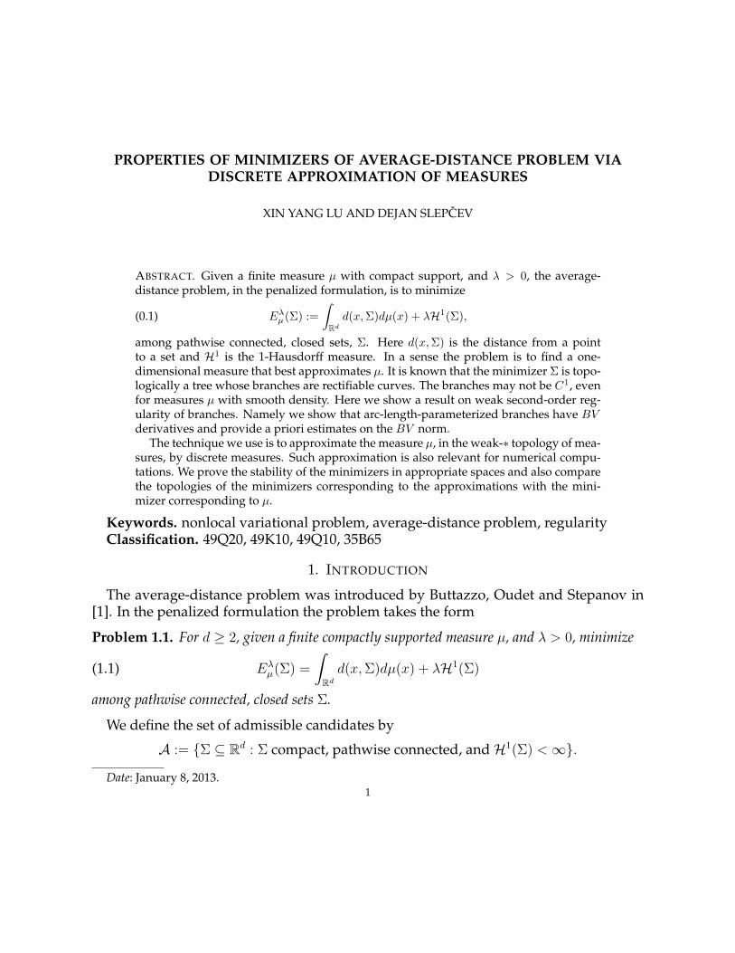
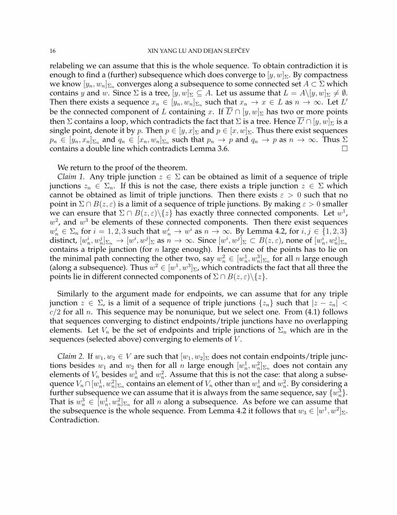
xn

vn

zw

qn

pn

Σn

Σ

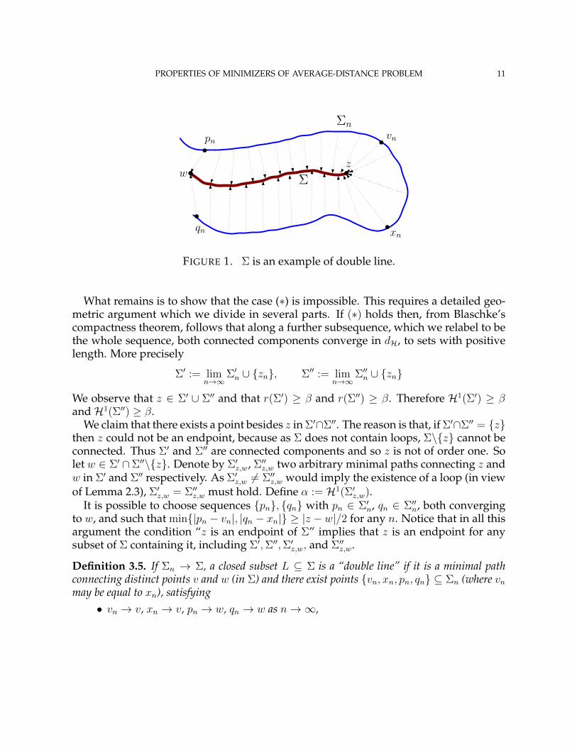
FIGURE 1. Σ is an example of double line.

What remains is to show that the case (∗) is impossible. This requires a detailed geo-metric argument which we divide in several parts. If (∗) holds then, from Blaschke’scompactness theorem, follows that along a further subsequence, which we relabel to bethe whole sequence, both connected components converge in dH, to sets with positivelength. More precisely

Σ′ := limn→∞

Σ′n ∪ {zn}, Σ′′ := limn→∞

Σ′′n ∪ {zn}

We observe that z ∈ Σ′ ∪ Σ′′ and that r(Σ′) ≥ β and r(Σ′′) ≥ β. Therefore H1(Σ′) ≥ βandH1(Σ′′) ≥ β.

We claim that there exists a point besides z in Σ′∩Σ′′. The reason is that, if Σ′∩Σ′′ = {z}then z could not be an endpoint, because as Σ does not contain loops, Σ\{z} cannot beconnected. Thus Σ′ and Σ′′ are connected components and so z is not of order one. Solet w ∈ Σ′ ∩Σ′′\{z}. Denote by Σ′z,w, Σ′′z,w two arbitrary minimal paths connecting z andw in Σ′ and Σ′′ respectively. As Σ′z,w 6= Σ′′z,w would imply the existence of a loop (in viewof Lemma 2.3), Σ′z,w = Σ′′z,w must hold. Define α := H1(Σ′z,w).

It is possible to choose sequences {pn}, {qn} with pn ∈ Σ′n, qn ∈ Σ′′n, both convergingto w, and such that min{|pn − vn|, |qn − xn|} ≥ |z − w|/2 for any n. Notice that in all thisargument the condition “z is an endpoint of Σ” implies that z is an endpoint for anysubset of Σ containing it, including Σ′,Σ′′,Σ′z,w, and Σ′′z,w.

Definition 3.5. If Σn → Σ, a closed subset L ⊆ Σ is a “double line” if it is a minimal pathconnecting distinct points v and w (in Σ) and there exist points {vn, xn, pn, qn} ⊆ Σn (where vnmay be equal to xn), satisfying

• vn → v, xn → v, pn → w, qn → w as n→∞,


• the minimal path between pn and qn contains {vn, xn} for any n.

It can be shown that, since Σ does not contain any loops, that if Σ has a double line,then it has a double line such that v is an endpoint. However we do not need this factin our arguments.

Notice that construction in case (∗) implies the presence of a double line in the limitset Σ.

Lemma 3.6. Given a sequence of discrete probability measures {µn} converging to some prob-ability measure µ w.r.t. weak-∗ topology, and a sequence of minimizers Σn ∈ argmin Eλ

µn

converging to Σ ∈ argmin Eλµ w.r.t. dH, then the set Σ cannot contain double lines.

Proof. The proof is done by contradiction: assume there exists a double line L ⊆ Σ. Theaim is to find a competitor Σn contradicting the optimality of Σn.

From the definition of a double line there exists distinct points v, w ∈ L and distinctpoints {vn, xn, pn, qn} ⊆ Σn for all n, satisfying

vn → v, xn → v, pn → w, qn → w as n→∞.

From the discussion above it is possible to choose these sequences such that thereexist disjoint curves γ′n, γ′′n : [0, 1] −→ Σn connecting pn to vn, and qn to xn respectively,and their respective image L′n, L′′n both converge to L w.r.t. dH. Let Ln := L′n ∪L′′n. It alsoholds that Σn\Ln ∪ L→ Σ w.r.t. dH as n→∞. By lower semicontinuity ofH1:

lim infn→∞

min{H1(L′n),H1(L′′n)} ≥ H1(L) ≥ dL(v, w) =: a > 0,

where dL denotes the path distance on L. It follows that lim infn→∞H1(Ln) ≥ 2H1(L) ≥2a, i.e. for n sufficiently largeH1(Ln) ≥ 1.9H1(L) holds.

Choose ε > 0, and n sufficiently large such that

max{dH(Σn,Σ), dH(Ln, L), dH(Σn\Ln ∪ L,Σ), |pn − w|, |qn − w|, |vn − v|} < ε.

Denote with [x, y] the line segment with endpoints in x and y. Define

An := (Σn\Ln) ∪ [pn, w] ∪ [qn, w] ∪ [vn, v] ∪ [xn, v] ∪ L,

i.e. An is obtained from Σn by first removing Ln and then replacing it with line segments[pn, w], [qn, w] [vn, v], [xn, v] and L. For any sets A,B ⊂ Rd we define

daH(A,B) = supb∈B

infa∈A|a− b|.

Note that dH(A,B) = max{daH(A,B), daH(B,A)}. Then daH(Σn, [pn, w]) ≤ |pn − w| < ε,and similarly daH(Σn, [qn, w]) < ε, daH(Σn, [vn, v]) < ε, daH(Σn, [xn, v]) < ε. Combining


with dH(Σn\Ln ∪ L,Σ) < ε gives daH(An,Σn) < ε. Moreover it holds

H1(An) ≤ H1(Σn)−H1(Ln) + |pn − w|+ |qn − w|+ |vn, v|+ [xn, v] +H1(L)

≤ H1(Σn)−H1(Ln) +H1(L) + 4ε

≤ H1(Σn)− 0.9H1(L) + 3ε

≤ H1(Σn)− 0.9a+ 3ε.

(3.1)

The issue we still face is that An may not belong to A. Namely An may be disconnected(for example if Ln contains triple junctions). Let Cn

0 be the connected component of Ancontaining L. Let Fn := {Cn

j }j∈I be the family of connected components of An, otherthan Cn

0 . Since each connected component must contain an endpoint of Σn, by Lemma3.1, I must be finite. We now translate these components so that they connect to L.Consider an arbitrary Cn

j ∈ Fn. As Ln is the only set present in Σn but not present inAn, there exists a point snj ∈ Ln ∩ Cn

j . Define

Tθ : Rd −→ Rd, Tθ(x) := x+ θ

the translation by a vector θ, and let πL be the projection on L, i.e. for any x the pointπL(x) satisfies |x− πL(x)| = d(x, L) (if there is more than one minimizer, then πL(x) canbe chosen arbitrarily among these). Define

Σn :=(An\

⋃j∈I

Cnj

)∪⋃j∈I

TπL(snj )−snj (Cnj ).

It is pathwise connected and compact by construction. Notice that dH(Ln, L) < ε implies|snj−πL(snj )| < ε. Therefore daH(Σn, An) ≤ ε, which combined with daH(An,Σn) < ε givesdaH(Σn,Σn) ≤ 2ε. From |d(x, Σn)−d(x,Σn)| ≤ daH(Σn,Σn) ≤ 2ε, integrating on Rd yields

(3.2)∣∣∣∣∫ d(x, Σn)dµn −

∫d(x,Σn)dµn

∣∣∣∣ ≤ µn(Rd)dH(Σn,Σn) ≤ 2ε.

The last step involves estimating H1(Σn): by construction Σn is obtained from An byfirst removing

⋃j∈I C

nj , then adding

⋃j∈I TπL(snj )−snj (Cn

j ). Since by definition Cnj ∩Cn

s = ∅if j 6= s and

⋃j∈I

Cnj ⊆ Σn,

H1(⋃j∈I

Cnj

)=∑j∈I

H1(Cnj ) ≤ H1(Σn) <∞.


Analogously, considering that TπL(snj )−snj (Cnj ) is the image of Cn

j through a translation,H1(TπL(snj )−snj (Cn

j )) = H1(Cnj ) for any j, thus

H1

(⋃j∈I

TπL(snj )−snj (Cnj )

)= H1

(⋃j∈I

Cnj

)=∑j∈I

H1(Cnj ) ≤ H1(Σn) <∞.

Using (3.1) this gives

H1(Σn) = H1(An) ≤ H1(Σn)− 0.9a+ 3ε.

Combining with (3.2) we conclude

Eλµn(Σn) ≤ Eλ

µn(Σn) + 2ε− 0.9λa+ 3ελ,

which for ε sufficiently small contradicts the minimality of Σn. �

We return to the proof of Theorem 3.4. It remains to consider the case that an endpointz ∈ ext(Σ) is a limit of points zn ∈ Σn of order 3. We note that arbitrarily close to anypoint of order 3 there exists a point of order 2. Thus z can be obtained as a limit of pointsof order 2, which is the case considered above. �

4. TOPOLOGICAL "LOWER SEMICONTINUITY"

4.1. Topological relation. Given λ > 0 and a compactly supported probability measureµ, consider a sequence of discrete probability measures {µn}

∗⇀µ, and for any n choose a

minimizer Σn ∈ argminEλµn . Then upon subsequence Σn

dH→Σ ∈ argminEλµ . The aim of

the this section is to analyze topological relations between Σn (for n sufficiently large)and Σ.

The main result is:

Theorem 4.1. Given λ > 0 and a compactly supported probability measure µ, consider asequence of discrete probability measures {µn}

∗⇀µ, and for any n choose a minimizer Σn ∈

argmin Eλµn . Then, upon a subsequence, Σn

dH→Σ ∈ argmin Eλµ . Then then for all sufficiently

large n along the subsequence there exists a homeomorphism ϕn : Σ −→ Sn ⊆ Σn, for somesubset Sn ⊆ Σn.

Proof. The convergence of Σn along a subsequence follows from Theorem 3.4. We againassume that the subsequence is the whole sequence. Let V be the set of all endpointsand triple junctions of Σ. By Theorem 3.4, Σ and Σn contain at most 1/λ endpoints.By induction on the number of triple junctions, it is easy to prove that in any tree thenumber of endpoints is greater than the number of triple junctions. Thus the number of


R

ϕ−1n

Σn

Σ

ϕn

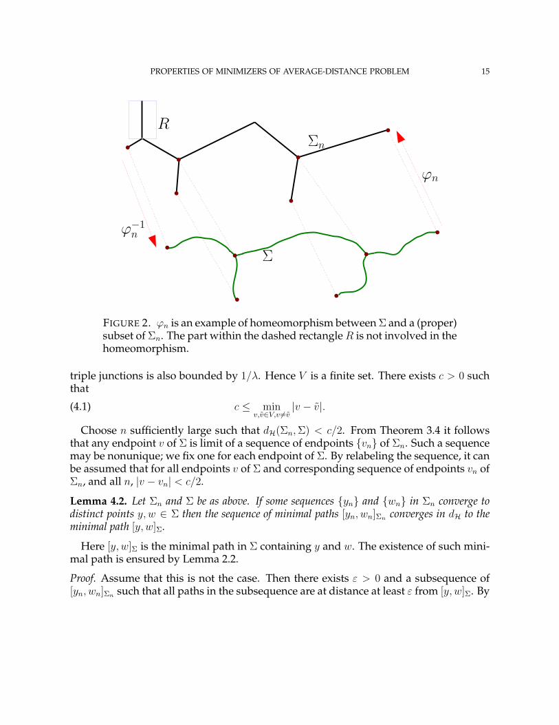
FIGURE 2. ϕn is an example of homeomorphism between Σ and a (proper)subset of Σn. The part within the dashed rectangleR is not involved in thehomeomorphism.

triple junctions is also bounded by 1/λ. Hence V is a finite set. There exists c > 0 suchthat

(4.1) c ≤ minv,v∈V,v 6=v

|v − v|.

Choose n sufficiently large such that dH(Σn,Σ) < c/2. From Theorem 3.4 it followsthat any endpoint v of Σ is limit of a sequence of endpoints {vn} of Σn. Such a sequencemay be nonunique; we fix one for each endpoint of Σ. By relabeling the sequence, it canbe assumed that for all endpoints v of Σ and corresponding sequence of endpoints vn ofΣn, and all n, |v − vn| < c/2.

Lemma 4.2. Let Σn and Σ be as above. If some sequences {yn} and {wn} in Σn converge todistinct points y, w ∈ Σ then the sequence of minimal paths [yn, wn]Σn converges in dH to theminimal path [y, w]Σ.

Here [y, w]Σ is the minimal path in Σ containing y and w. The existence of such mini-mal path is ensured by Lemma 2.2.

Proof. Assume that this is not the case. Then there exists ε > 0 and a subsequence of[yn, wn]Σn such that all paths in the subsequence are at distance at least ε from [y, w]Σ. By


relabeling we can assume that this is the whole sequence. To obtain contradiction it isenough to find a (further) subsequence which does converge to [y, w]Σ. By compactnesswe know [yn, wn]Σn converges along a subsequence to some connected set A ⊂ Σ whichcontains y and w. Since Σ is a tree, [y, w]Σ ⊆ A. Let us assume that L = A\[y, w]Σ 6= ∅.Then there exists a sequence xn ∈ [yn, wn]Σn such that xn → x ∈ L as n → ∞. Let L′

be the connected component of L containing x. If L′ ∩ [y, w]Σ has two or more pointsthen Σ contains a loop, which contradicts the fact that Σ is a tree. Hence L′ ∩ [y, w]Σ is asingle point, denote it by p. Then p ∈ [y, x]Σ and p ∈ [x,w]Σ. Thus there exist sequencespn ∈ [yn, xn]Σn and qn ∈ [xn, wn]Σn such that pn → p and qn → p as n → ∞. Thus Σcontains a double line which contradicts Lemma 3.6. �

We return to the proof of the theorem.Claim 1. Any triple junction z ∈ Σ can be obtained as limit of a sequence of triple

junctions zn ∈ Σn. If this is not the case, there exists a triple junction z ∈ Σ whichcannot be obtained as limit of triple junctions. Then there exists ε > 0 such that nopoint in Σ ∩ B(z, ε) is a limit of a sequence of triple junctions. By making ε > 0 smallerwe can ensure that Σ ∩ B(z, ε)\{z} has exactly three connected components. Let w1,w2, and w3 be elements of these connected components. Then there exist sequenceswin ∈ Σn for i = 1, 2, 3 such that win → wi as n → ∞. By Lemma 4.2, for i, j ∈ {1, 2, 3}distinct, [win, w

jn]Σn → [wi, wj]Σ as n → ∞. Since [wi, wj]Σ ⊂ B(z, ε), none of [win, w

jn]Σn

contains a triple junction (for n large enough). Hence one of the points has to lie onthe minimal path connecting the other two, say w2

n ∈ [w1n, w

3n]Σn for all n large enough

(along a subsequence). Thus w2 ∈ [w1, w3]Σ, which contradicts the fact that all three thepoints lie in different connected components of Σ ∩B(z, ε)\{z}.

Similarly to the argument made for endpoints, we can assume that for any triplejunction z ∈ Σ, is a limit of a sequence of triple junctions {zn} such that |z − zn| <c/2 for all n. This sequence may be nonunique, but we select one. From (4.1) followsthat sequences converging to distinct endpoints/triple junctions have no overlappingelements. Let Vn be the set of endpoints and triple junctions of Σn which are in thesequences (selected above) converging to elements of V .

Claim 2. If w1, w2 ∈ V are such that [w1, w2]Σ does not contain endpoints/triple junc-tions besides w1 and w2 then for all n large enough [w1

n, w2n]Σn does not contain any

elements of Vn besides w1n and w2

n. Assume that this is not the case: that along a subse-quence Vn∩ [w1

n, w2n]Σn contains an element of Vn other than w1

n and w2n. By considering a

further subsequence we can assume that it is always from the same sequence, say {w3n}.

That is w3n ∈ [w1

n, w2n]Σn for all n along a subsequence. As before we can assume that

the subsequence is the whole sequence. From Lemma 4.2 it follows that w3 ∈ [w1, w2]Σ.Contradiction.


We are finally ready to define the desired homeomorphism. Choose a function ϕn :Σ −→ ϕn(Σ) ⊆ Σn such that:

(i) if an endpoint v ∈ Σ is limit of a sequence of endpoints {vn} with vn ∈ Vn thenϕn(v) = vn,

(ii) if a triple junction z ∈ Σ is limit of a sequence of triple junctions {zn}with zn ∈ Vn,then ϕn(z) = zn,

(iii) if w1, w2 ∈ V are such that [w1, w2]Σ does not contain endpoints/triple junctionsbesides w1, w2, then define ϕn|[w1,w2]Σ as an arbitrary homeomorphism between[w1, w2]Σ and [w1

n, w2n]Σn , where w1

n, w2n ∈ Vn and {w1

n} → w1, {w2n} → w2, as n→∞.

The function ϕn : Σ → ϕn(Σ) ⊆ Σn is well defined, for n large enough, by Claim 2.It is injective and continuous by construction. Since Σ is compact and ϕn is a bijection,ϕ−1n is continuous. Thus ϕn is a homeomorphism. �

5. BV ESTIMATES

The aim of this section is to prove a regularity result about minimizers of Problem 1.1.In [1], [2] and [3] is has been proven that any minimizer Σ of Problem 1.1 is a countableunion of Lipschitz curves. Given that, by Theorem 3.4, the total mass arriving at eachendpoint is at least λ there exists at most 1/λ endpoints. Since the number of triplejunctions in a tree is less than the number of endpoints the number of curves, formingthe tree, is bounded by 1/λ. Thus Σ is a finite union of Lipschitz curves.

The main objective of this section is to prove the following regularity result:

Theorem 5.1. Given a compactly supported finite measure µ, and λ > 0, any Σ ∈ argmin Eλµ

is finite union of Lipschitz curves {γk}Nk=1 (without loss of generality assume that all γk arearc-length parameterized), such that∑

k

‖γ′k‖TV ≤1

λ|µ(Rd)|,

where ‖ · ‖TV denotes the total variation.

Note that we do not assume that µ is a probability measure.The proof uses a discrete approximation of µ; thus we start by proving the result for

discrete measures. Given unit vectors v1, and v2, the "angle between” v1 and v2 is definedas the smallest α ≥ 0 such that

|v1 − v2| = 2 sinα

2.

Lemma 5.2. Given an arbitrary discrete measure µ, and λ > 0, any Σ ∈ argmin Eλµ is finite

union of Lipschitz curves {γk}Nk=1 (without loss of generality assume γk constant speed), such


that‖γ′k‖TV ≤

1

λσ(µ,Σ, γk)

where σ is defined after Lemma 2.1.

Proof. Let µ be a probability measure. The result for general measures follows by scal-ing (See Section 2.1 in [10]). Consider an arbitrary minimizer Σ ∈ argmin Eλ

µ . From[10] follows that minimizers are always Steiner graphs with finitely many vertices. AsSteiner graphs are trees, it follows that Σ is finite union of arc-length parameterized Lip-schitz curves {γk}Nk=1, where each of these curves is union of line segments. Moreover,the number of curves, N , is bounded by 1/λ. Choose an arbitrary k ∈ {1, · · · , N}. Tosimplify notations define γ := γk and L := H1(γ). Let s1 < s2 < · · · < sm be the valuesin [0, L] for which γ(si) is a corner.

From definition of total variation and the fact that the curve is piecewise linear

‖γ′‖TV ([0,L]) := sup0=t0<t1<···<tM−1<tM=L

M−1∑i=0

|γ′(ti+1)− γ′(ti)| =m∑j=1

|γ′(sj−)− γ′(sj+)|

where γ′(·−) and γ′(·+) denote the left and the right derivative respectively.From the proof of Lemma 11 in [10] follows that

m∑j=1

|γ′(sj−)− γ′(sj+)| ≤ 1

λσ(µ,Σ, γ).

We should note that Lemma 11 of [10] is stated for probability measures. However it isstraightforward to extend the proof to include arbitrary discrete measures, in particularin the light of the scaling presented in Section 2.1 of [10].

The inequalities above imply the desired estimate on total variation. �

We remark that combining the estimate on the total variation above and the estimate(2.1) onH1(Σ) we obtain an estimate on the BV norm

N∑k=1

‖γk‖BV ≤1

λ(|µ(Rd)|+ diam suppµ).

Proof. (of Theorem 5.1) As in the proof of the lemma we assume that µ is a probabilitymeasure, as the general result follows by scaling. In [1], [2] and [3] (to which we refer forfurther details) it has been proven that minimizers of the average-distance functional areat most countable unions of Lipschitz curves, for the constrained formulation. It easyto notice that each minimizer Σ ∈ argmin Eλ

µ is a minimizer of minH1(X )≤H1(Σ) Fµ(X )

too. In Lemma 3.1 it has been proven that minimizer Σ ∈ argmin Eλµ has at most 1/λ

endpoints, thus Σ is finite union of Lipschitz curves.


For BV regularity, consider an arbitrary minimizer Σ ∈ argmin Eλµ . If we consider

discrete approximations of µ and the corresponding minimizers Σn then, as before, Σn

converge along a subsequence to some Σ ∈ argmin Eλµ . The problem, we need to over-

come, is that Σ may be different from Σ, as the minimizer is not unique in general. Notethat if Σ ⊆ Σ then there is no problem since the regularity of Σ implies the regularity ofΣ.

Thus we modify the measure µ in such a way that Σ is still a minimizer of the energycorresponding to the modified measure, but that ensures that any minimizer of the en-ergy corresponding to the modified measure contains Σ. This is one of the key ideas ofthe paper. In particular let ε > 0 and

µε := µ+ ε1

H1(Σ)H1|Σ.

Note that Σ is the minimal (w.r.t. set inclusion) minimizer of Eλµε for any ε > 0, i.e. every

minimizer Σ′ ∈ argmin Eλµε contains Σ. Indeed, as Σ is already a minimizer of Eλ

µ , givenan arbitrary element Σ′ ∈ A it holds that Eλ

µ(Σ) ≤ Eλµ(Σ′). Hence if Σ′ is a minimizer of

Eλµε then

∫Σd(x,Σ′)dH1

|Σ = 0 and thus Σ ⊆ Σ′.Fix ε > 0, and choose an approximating sequence {µn}

∗⇀µε, where µn is a discrete

measure with µn(Rd) = µε(Rd) = 1 + ε. For any n choose Σn ∈ argmin Eλµn . Upon a

subsequence (which we can assume to be the whole sequence), ΣndH→Σ∗ ∈ argmin Eλ

µε ,which implies Σ ⊆ Σ∗.

We know that Σ∗ is a union of Lipschitz curves {γ∗,i : i = 1, . . . , N} such that end-points of all curves are either endpoints or triple junctions of Σ∗. By Lemma 4.2 and theproof of Theorem 4.1 for each n large enough there exist curves, {γni : i = 1, . . . , N, n ≥n0}, with disjoint interiors in Σn such that for each i, γni → γ∗,i in dH as n → ∞. Notethat Lemma 5.2 gives

(5.1)N∑i=1

‖(γni )′‖TV ≤1 + ε

λ.

Since the H1(Σn) are uniformly bounded∑N

i=1 ‖(γni )′‖BV are also uniformly bounded.The estimates of Lemma 5.2 and fact (v) from the introduction (which relies on the factthat BV is compactly embedded in L1) imply that along a subsequence (γni )′ → γ′∗,i inL1 as n→∞.

Since total variation is lower semicontinuous with respect to L1 convergence we con-clude that for all i = 1, . . . , N

lim infn→∞

‖(γni )′‖TV ≥ ‖γ′∗,i‖TV .


Combining with (5.1), and using the lower-semicontinuity ofH1 with respect to L1 con-vergence of γni , we obtain

N∑i=1

‖(γ∗,i)′‖TV ≤1 + ε

λ.

Since the curves that make up Σ are subsets of the curves that make up Σ∗ we conclude:N∑i=1

‖(γi)′‖TV ≤1 + ε

λ.

Taking ε→ 0 yields the desired result. �

Again by combining the estimate on the total variation above and the estimate (2.1)onH1(Σ) one obtains

N∑k=1

‖γk‖BV ≤1

λ(|µ(Rd)|+ diam suppµ).

Acknowledgments. XYL acknowledges the support by ICTI. DS is grateful to NSF(grants DMS-0908415 and DMS-1211760) and FCT (grant UTA_CMU/MAT/0007/2009).Authors are thankful to the Center for Nonlinear Analysis (NSF grant DMS-0635983) forits support. The research was also supported by NSF PIRE grant OISE-0967140.

REFERENCES

[1] BUTTAZZO, G., OUDET, E., and STEPANOV, E.: Optimal transportation problems with free Dirichletregions , Progress in Nonlinear Diff. Equations and their Applications vol. 51, pp. 41-65, 2002

[2] BUTTAZZO, G. and STEPANOV, E.: Minimization problems for average distance functionals, Calculus ofVariations: Topics from the Mathematical Heritage of Ennio De Giorgi, D. Pallara (ed.), Quaderni diMatematica, Seconda Università di Napoli, Caserta vol. 14, pp. 47-83, 2004

[3] BUTTAZZO, G. and STEPANOV, E.: Optimal transportation networks as free Dirichlet regions for theMonge-Kantorovich problem, Ann. Sc. Norm. Sup. Pisa Cl. Sci. vol. 2, pp. 631-678, 2003

[4] GILBERT, E.N. and POLLACK, H.O.: Steiner minimal trees, SIAM J. Appl. Math., vol 12, pp. 1-29, 1968[5] HWANG, F.K., RICHARDS, D.S. and WINTER, P.: The Steiner tree problem, vol. 53 of Annals of Discrete

Mathematics, North-Holland Publishing Co., Amsterdam, 1992[6] LEMENANT, A.: A presentation of the average distance minimizing problem, POMI, vol. 390, pp. 117-146,

2011[7] LEMENANT, A.: About the regularity of average distance minimizers in R2, Preprint,[8] MANTEGAZZA, C. and MENNUCCI, A.: Hamilton-jacobi equations and distance functions in Riemannian

manifolds , Appl. Math. Optim., vol. 47(1), pp. 1-25, 2003[9] PAOLINI E. and STEPANOV E.: Qualitative properties of maximum and average distance minimizers in Rn,

J. of Math. Sci. (N. Y.), vol. 122(3), pp. 3290-3309, 2004[10] SLEPCEV, D.: Counterexample to regularity in average-distance problem, Preprint

(available at http://www.math.cmu.edu/users/slepcev/adp1.pdf)


[11] SANTAMBROGIO, F. and TILLI, P.: Blow-up of Optimal Sets in the Irrigation Problem, J. Geom. Anal.,vol. 15(2), pp. 343-362, 2005

[12] TILLI, P.: Some explicit examples of minimizers for the irrigation problem, J. Convex Anal., vol. 17, pp.583-595, 2010

DEPARTMENT OF MATHEMATICAL SCIENCES, CARNEGIE MELLON UNIVERSITY, PITTSBURGH, PA,15213,UNITED STATES, EMAILS: [email protected], [email protected]

PROPERTIES OF MINIMIZERS OF AVERAGE-DISTANCE … · properties of minimizers of average-distance...

Documents

Transcript of PROPERTIES OF MINIMIZERS OF AVERAGE-DISTANCE … · properties of minimizers of average-distance...