Project work: Implementation and run-time mesh re nement ... · Project work: Implementation and...
65
CFD with OpenSource software A course at Chalmers University of Technology Taught by H˚ akan Nilsson Project work: Implementation and run-time mesh refinement for the k - ω SST DES turbulence model when applied to airfoils. Developed for OpenFOAM-2.2.x Author: Daniel Lindblad Peer reviewed by: Adam Jareteg Olivier Petit Disclaimer: This is a student project work, done as part of a course where OpenFOAM and some other OpenSource software are introduced to the students. Any reader should be aware that it might not be free of errors. Still, it might be useful for someone who would like learn some details similar to the ones presented in the report and in the accompanying files. The material has gone through a review process. The role of the reviewer is to go through the tutorial and make sure that it works, that it is possible to follow, and to some extent correct the writing. The reviewer has no responsibility for the contents. January 25, 2014
-
Upload
nguyentruc -
Category
Documents
-
view
215 -
download
0
Transcript of Project work: Implementation and run-time mesh re nement ... · Project work: Implementation and...
CFD with OpenSource software
A course at Chalmers University of TechnologyTaught by Hakan Nilsson
Project work:
Implementation and run-time meshrefinement for the k − ω SST DES
turbulence model when applied to airfoils.
Developed for OpenFOAM-2.2.x
Author:Daniel Lindblad
Peer reviewed by:Adam JaretegOlivier Petit
Disclaimer: This is a student project work, done as part of a course where OpenFOAM and someother OpenSource software are introduced to the students. Any reader should be aware that it
might not be free of errors. Still, it might be useful for someone who would like learn some detailssimilar to the ones presented in the report and in the accompanying files. The material has gone
through a review process. The role of the reviewer is to go through the tutorial and make sure thatit works, that it is possible to follow, and to some extent correct the writing. The reviewer has no
responsibility for the contents.
January 25, 2014
Contents
1 Introduction 3
2 Theory 42.1 The k − ω SST DES turbulence model . . . . . . . . . . . . . . . . . . . . . . . . . . 4
2.1.1 Short background . . . . . . . . . . . . . . . . . . . . . . . . . . . . . . . . . 42.1.2 Governing transport equations . . . . . . . . . . . . . . . . . . . . . . . . . . 4
2.2 Boundary conditions . . . . . . . . . . . . . . . . . . . . . . . . . . . . . . . . . . . . 72.3 Applying run-time mesh refinement . . . . . . . . . . . . . . . . . . . . . . . . . . . . 9
3 The OpenFOAM implementation 113.1 k − ω SST SAS model . . . . . . . . . . . . . . . . . . . . . . . . . . . . . . . . . . . 11
3.1.1 kOmegaSSTSAS.H . . . . . . . . . . . . . . . . . . . . . . . . . . . . . . . . . 113.1.2 kOmegaSSTSAS.C . . . . . . . . . . . . . . . . . . . . . . . . . . . . . . . . . 14
3.2 pimpleDyMFoam . . . . . . . . . . . . . . . . . . . . . . . . . . . . . . . . . . . . . . 213.2.1 Comparison between pimpleFoam.C and pimpleDyMFoam.C . . . . . . . . . 223.2.2 Mesh refinement in pimpleDyMFoam . . . . . . . . . . . . . . . . . . . . . . . 243.2.3 Suggested modifications for mesh refinement . . . . . . . . . . . . . . . . . . 31
4 Implementing k − ω SST DES 334.1 k − ω SST DES . . . . . . . . . . . . . . . . . . . . . . . . . . . . . . . . . . . . . . . 33
4.1.1 Copying the kOmegaSSTSAS model . . . . . . . . . . . . . . . . . . . . . . . 334.1.2 Creating the class kOmegaSSTDES . . . . . . . . . . . . . . . . . . . . . . . 334.1.3 Modifying kOmegaSSTDES.H . . . . . . . . . . . . . . . . . . . . . . . . . . 354.1.4 Modifying kOmegaSSTDES.C . . . . . . . . . . . . . . . . . . . . . . . . . . . 37
4.2 k − ω SST DES Refine . . . . . . . . . . . . . . . . . . . . . . . . . . . . . . . . . . . 414.2.1 Creating the class kOmegaSSTDESRefine . . . . . . . . . . . . . . . . . . . . 424.2.2 Modifying kOmegaSSTDESRefine.H . . . . . . . . . . . . . . . . . . . . . . . 434.2.3 Modifying kOmegaSSTDESRefine.C . . . . . . . . . . . . . . . . . . . . . . . 44
5 Simulation with mesh refinement 475.1 Copying files . . . . . . . . . . . . . . . . . . . . . . . . . . . . . . . . . . . . . . . . 475.2 Creating the mesh . . . . . . . . . . . . . . . . . . . . . . . . . . . . . . . . . . . . . 485.3 The 0/ directory . . . . . . . . . . . . . . . . . . . . . . . . . . . . . . . . . . . . . . 49
5.3.1 Velocity . . . . . . . . . . . . . . . . . . . . . . . . . . . . . . . . . . . . . . . 495.3.2 Pressure . . . . . . . . . . . . . . . . . . . . . . . . . . . . . . . . . . . . . . . 505.3.3 Turbulent kinetic energy . . . . . . . . . . . . . . . . . . . . . . . . . . . . . . 505.3.4 Turbulent frequency . . . . . . . . . . . . . . . . . . . . . . . . . . . . . . . . 515.3.5 Turbulent/Sub grid scale viscosity . . . . . . . . . . . . . . . . . . . . . . . . 525.3.6 LDES/LDDES . . . . . . . . . . . . . . . . . . . . . . . . . . . . . . . . . . . 52
5.4 The dictionaries . . . . . . . . . . . . . . . . . . . . . . . . . . . . . . . . . . . . . . . 535.4.1 controlDict . . . . . . . . . . . . . . . . . . . . . . . . . . . . . . . . . . . . . 535.4.2 fvSolution . . . . . . . . . . . . . . . . . . . . . . . . . . . . . . . . . . . . . . 545.4.3 fvSchemes . . . . . . . . . . . . . . . . . . . . . . . . . . . . . . . . . . . . . . 55
1
CONTENTS CONTENTS
5.4.4 LESProperties . . . . . . . . . . . . . . . . . . . . . . . . . . . . . . . . . . . 565.4.5 dynamicMeshDict . . . . . . . . . . . . . . . . . . . . . . . . . . . . . . . . . 56
5.5 Running the case . . . . . . . . . . . . . . . . . . . . . . . . . . . . . . . . . . . . . . 575.5.1 Without refinement . . . . . . . . . . . . . . . . . . . . . . . . . . . . . . . . 575.5.2 Enabling refinement . . . . . . . . . . . . . . . . . . . . . . . . . . . . . . . . 58
6 Conclusions 60
A MATLAB program to generate airfoil geometry 62
B Extension of blockMeshDict for 3D simulation 63
2
Chapter 1
Introduction
This is a report for a project in the course ”CFD with OpenSource software”, given by Hakan Nilssonin the autumn of 2013 at Chalmers University of Technology. The work is developed for OpenFOAM2.2.x.
In this project, the k−ω SST DES turbulence model [1] is going to be implemented and investi-gated when applied to airfoil simulations. In addition to this, run-time mesh refinement features inOpenFOAM 2.2.x. will be investigated and applied to the simulations using the dynamicRefineFvMeshclass and the pimpleDyMFoam solver.
The k−ω SST DES turbulence model is based upon the turbulence model k−ω SST, which is aneddy viscosity model developed for aeronautic flows with pressure induced separation and adversepressure gradient flows [1]. The model is then equipped with what is known as DES features,where DES stands for Detached Eddy Simulations. The main goal of this approach is to reduce theturbulent viscosity in regions where the mesh is fine enough to resolve large turbulent structures,and hence do LES here. Therefore the model can be viewed as a trade off between LES and URANS,with a computational cost in between the two.
In OpenFOAM, two implementations based upon the k− ω SST model are found. The first is afurther developed version of the original k − ω SST model, in which additional changes have beenmade for various purposes. This is a RAS turbulence model, i.e. designed to be used for RANS orURANS simulations in which all of the turbulence is modeled. Next there is an implementation ofthe k − ω SST SAS model presented in [2], where SAS stands for Scale Adaptive Simulation. It isbased upon the original k − ω SST model in which SAS features have been introduced in an extrasource term in the ω equation. Since it is only different from the k−ω SST DES model with respectto one source term, see [1] and [2], it will serve as the base for the DES implementation.
Since DES models are designed to resolve turbulence where the grid is fine enough, this allowsfor the user to control where turbulence is to be resolved and when it is not. One way to do this isto refine the mesh run-time in desired regions until the model starts resolving turbulence in theseregions. This is the second part of the project.
A test case is set to be cambered NACA four digit airfoil in 2 and 3D. The surface shape isgenerated according to the NACA four digit standard, and a Fortran routine found at [3] is used tothen create a blockMesh dictionary. Since three dimensional simulations are very computer intensivewhen finer grids are employed, it is mainly the focus to run the case in 2D during development andvalidation.
3
Chapter 2
Theory
In this chapter the k − ω SST DES turbulence model which will be implemented in OpenFOAM ispresented. The boundary conditions employed will also be presented as well as a short overview ofhow the mesh refinement will be controlled.
2.1 The k − ω SST DES turbulence model
2.1.1 Short background
The k − ω SST-DES model is a DES modification of the RANS model k − ω SST. The standardSST model is a mix between the k− ε and the k−ω model, in which the former is used in the outerpart of the boundary layer as well as outside of it, and the latter in the inner part of the boundarylayer [1]. The transport equation for ε in the k− ε model is however rewritten as an equation for ω,giving a similar equation to the original ω equation but with some additional terms and constants.This does however allow the computer to only solve for one pair of transport equations and theswitching between the two formulations is done by so called blending functions. The advantage ofusing different models in different regions is that the two models have their individual strengthsand weaknesses. The k − ω model is a low Reynolds number model, which means that it does notneed extra damping functions to ensure correct behavior close to walls. On the other hand the ωequation shows great sensitivity to free stream values of ω [1]. These two features are not presentin the k− ε model, i.e. it is not a low Reynolds number model and neither is it sensitive to the freestream values of k or ε.
Apart from this combination of features, the k−ω SST model has been equipped with additionalfeatures over its two base models. The first feature is a shear stress limiter (reducing νt), whichensures that the turbulent shear stress does not become too large in adverse pressure gradient regions,typically found on the top of an airfoil. Also a production limiter is applied on the production termin the k equation in order to prevent build up of turbulence in stagnant regions [1].
The model has finally been equipped with DES features, which aims at reducing the turbulentviscosity in regions where the mesh is sufficiently fine. This means that the model effectively transfersfrom RANS mode to LES mode in these regions, and the turbulent viscosity should be viewed as asub grid scale viscosity instead.
Since the introduction of the k−ω SST model it has undergone some changes in its formulation.The aim of the following section is therefore both to give an understanding of how the model worksas well as to show exactly which model that will be implemented in OpenFOAM.
2.1.2 Governing transport equations
The definition of ω in terms of k and ε reads
ω =ε
β∗k, β∗ = Cµ. (2.1)
4
2.1. THE K − ω SST DES TURBULENCE MODEL CHAPTER 2. THEORY
Here Cµ is the constant present in the expression for the turbulent viscosity in the k − ε model,and it is equal to 0.09. This definition is used to rewrite the transport equation for ε as a transportequation for ω, a derivation that will not be presented here.
The modeled transport equation for the turbulent kinetic energy, k, used in k − ω SST DESmodel reads, see [1], [2]
∂k
∂t+∂(uik)
∂xi= Pk +
∂
∂xi
[(ν +
νtσk
)∂k
∂xi
]− β∗kωFDES . (2.2)
It is the modified production Pk as well as the term FDES that differ this transport equation fromthose found in the base models. The bar over the velocity is indicating that the velocity field isfiltered in the sense that not all turbulent fluctuations are resolved. In URANS regions, this wouldcorrespond to a time filter, and in LES regions a space filter. This is however just a formality, sinceno actual filtering is done in the solver. Next the transport equation for ω reads [1], [2]
∂ω
∂t+∂(uiω)
∂xi= Pω +
∂
∂xi
[(ν +
νtσω
)∂ω
∂xi
]− βω2
+2(1− F1)σω21
ω
∂k
∂xi
∂ω
∂xi. (2.3)
The last cross diffusion term stems from the k − ε model when formulated as a k − ω model andhence should only be active away from the wall. Now, to begin with, the production term in the ωequation is evaluated as [1]
Pω = αS2, (2.4)
where S =√
2sij sij is the invariant measure of the strain rate [1] and
sij =1
2
(∂ui∂xj
+∂uj∂xi
), (2.5)
is the strain rate tensor of the filtered velocity field. Next we have the first blending function, F1,which is evaluated as [1], [2]
F1 = tanh(ξ4), ξ = min
[max
( √k
β∗ωy,
500ν
y2ω
),
4σω2k
CDωy2
]. (2.6)
Its purpose is to switch the SST model between the k−ω and k−ε formulation by changing betweenthe value 1 close to the wall, to 0 in the outer part of the boundary layer as well as outside of it. Itappears in the ω equation (2.3) in the last term, and hence can be seen to activate this term whenit goes to 0, giving the k − ε formulation instead. The model constants α, β, σk and σω are in factalso blended between the two formulations to give model constants applicable for the formulationused in a certain region. This is done according to
φ = F1φ1 + (1− F1)φ2, (2.7)
when φi denotes either αi or βi, or according to
1
ψ= F1
1
ψ1+ (1− F1)
1
ψ2, (2.8)
when ψj denotes either σkj or σωj . The values of the constants are taken from [1]
α1 = 5/9, α2 = 0.44,
β1 = 3/40, β2 = 0.0828,
1
σk1= 0.85, 1
σk2= 1,
1
σω1= 0.5, 1
σω2= 0.856.
5
2.1. THE K − ω SST DES TURBULENCE MODEL CHAPTER 2. THEORY
These constants are in fact derived from the original constants of the k − ε and k − ω models.Furthermore, CDω stems from the cross diffusion term in (2.3) and is defined by, see [1]
CDω = max
(2σω2
1
ω
∂k
∂xi
∂ω
∂xi, 10−10
). (2.9)
The SST model also features a shear stress limiter, which will switch from a eddy viscosity model tothe Johnson King model in regions where the shear stress becomes too large, i.e. adverse pressuregradient flow. It is defined as [1]
νt =a1k
max(a1ω, SF2), (2.10)
where a1 =√β∗ and F2 is another blending function that ensures that the Johnson King model
only can be active in the boundary layer. It is defined as
F2 = tanh(η2), η = max
(2√k
β∗ωy,
500ν
y2ω
). (2.11)
It should be mentioned that throughout, y denotes the distance to the closest wall. The productionof turbulent kinetic energy features a limiter and is defined as [1]
Pk = min(Pk, 10 · β∗kω),
Pk = νt
(∂ui∂xj
+∂uj∂xi
)∂ui∂xj
. (2.12)
It now remains to show how the DES features are incorporated. In the dissipation term of the kequation, the function FDES is included. In the original k − ω SST model the dissipation is notmultiplied by this term, which reads [1]
FDES = max
(Lt
CDES∆, 1
)(2.13)
Where Lt =√k/(β∗ω) is a turbulent length scale, ∆ = max(∆x1,∆x2,∆x3) is the largest side of
a cell at the present point in the grid and CDES = 0.61. When the local grid is fine enough in alldirections, compared to the turbulent length scale, the FDES term grows larger than 1. This willin turn reduce k, which reduces νt, see (2.10), and hence allows the solution to go unsteady. Thusin regions where the mesh is fine enough to resolve turbulence, the model will reduce the amountof modeled turbulent shear stress and allow the region to be treated with LES. There is however aproblem with this formulation when it comes to near wall regions. Since the grid generally is fineclose to walls, it could happen that the solution is triggered to go unsteady here. This is generallya bad result since near wall turbulent structures are very small and require a very fine grid to beresolved properly with LES. These requirements might not be satisfied by the mesh and hence apoorly resolved LES simulation close to the walls might be the result. Therefore the model is alsopresented with DDES (Delayed Detached Eddy Simulations) features, which protects it from goingunsteady near the wall. In this case the FDES term is modified according to
FDDES = max
(Lt
CDES∆(1− FS), 1
)(2.14)
in which FS is a blending function, chosen as either F1 or F2. As can be seen, the blending functionwill ensure that the term is reduced in the boundary layer, since the blending function becomes closeto 1 here.
6
2.2. BOUNDARY CONDITIONS CHAPTER 2. THEORY
2.2 Boundary conditions
Indeed, for any CFD simulation, the boundary treatment is important in order to get accurate andreliable results. As mentioned earlier, the k − ω SST model is a blend of the k − ε and the k − ωwith some additional features. One reason for this is that the k−ω model shows great sensitivity tothe free stream values of ω whereas it behaves much better in the near wall regions than the k − εmodel [1]. In addition to this, advanced wall treatment for ω has also been developed in order tomake it less sensitive to near wall grid resolution, see [1] and [4].
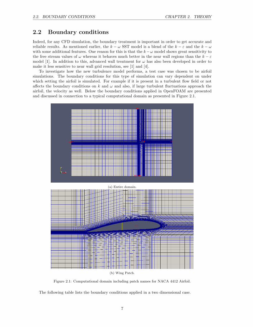
To investigate how the new turbulence model performs, a test case was chosen to be airfoilsimulations. The boundary conditions for this type of simulation can vary dependent on underwhich setting the airfoil is simulated. For example if it is present in a turbulent flow field or notaffects the boundary conditions on k and ω and also, if large turbulent fluctuations approach theairfoil, the velocity as well. Below the boundary conditions applied in OpenFOAM are presentedand discussed in connection to a typical computational domain as presented in Figure 2.1.
(a) Entire domain.
(b) Wing Patch.
Figure 2.1: Computational domain including patch names for NACA 4412 Airfoil.
The following table lists the boundary conditions applied in a two dimensional case.
7
2.2. BOUNDARY CONDITIONS CHAPTER 2. THEORY
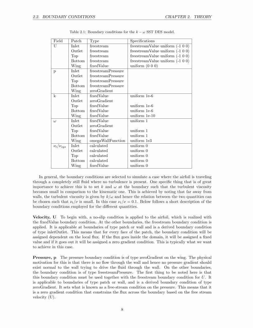
Table 2.1: Boundary conditions for the k − ω SST DES model.
Field Patch Type SpecificationsU Inlet freestream freestreamValue uniform (-1 0 0)
Outlet freestream freestreamValue uniform (-1 0 0)Top freestream freestreamValue uniform (-1 0 0)Bottom freestream freestreamValue uniform (-1 0 0)Wing fixedValue uniform (0 0 0)
p Inlet freestreamPressureOutlet freestreamPressureTop freestreamPressureBottom freestreamPressureWing zeroGradient
k Inlet fixedValue uniform 1e-6Outlet zeroGradientTop fixedValue uniform 1e-6Bottom fixedValue uniform 1e-6Wing fixedValue uniform 1e-10
ω Inlet fixedValue uniform 1Outlet zeroGradientTop fixedValue uniform 1Bottom fixedValue uniform 1Wing omegaWallFunction uniform 1e3
νt/νsgs Inlet calculated uniform 0Outlet calculated uniform 0Top calculated uniform 0Bottom calculated uniform 0Wing fixedValue uniform 0
In general, the boundary conditions are selected to simulate a case where the airfoil is travelingthrough a completely still fluid where no turbulence is present. One specific thing that is of greatimportance to achieve this is to set k and ω at the boundary such that the turbulent viscositybecomes small in comparison to the kinematic one. This is achieved by noting that far away fromwalls, the turbulent viscosity is given by k/ω and hence the relation between the two quantities canbe chosen such that νt/ν is small. In this case νt/ν = 0.1. Below follows a short description of theboundary conditions employed for the different quantities.
Velocity, U To begin with, a no-slip condition is applied to the airfoil, which is realized withthe fixedValue boundary condition. At the other boundaries, the freestream boundary condition isapplied. It is applicable at boundaries of type patch or wall and is a derived boundary conditionof type inletOutlet. This means that for every face of the patch, the boundary condition will beassigned dependent on the local flux. If the flux goes inside the domain, it will be assigned a fixedvalue and if it goes out it will be assigned a zero gradient condition. This is typically what we wantto achieve in this case.
Pressure, p The pressure boundary condition is of type zeroGradient on the wing. The physicalmotivation for this is that there is no flow through the wall and hence no pressure gradient shouldexist normal to the wall trying to drive the fluid through the wall. On the other boundaries,the boundary condition is of type freestreamPressure. The first thing to be noted here is thatthis boundary condition must be used together with the freestream boundary condition for U . Itis applicable to boundaries of type patch or wall, and is a derived boundary condition of typezeroGradient. It sets what is known as a free-stream condition on the pressure. This means that itis a zero gradient condition that constrains the flux across the boundary based on the free streamvelocity (U).
8
2.3. APPLYING RUN-TIME MESH REFINEMENT CHAPTER 2. THEORY
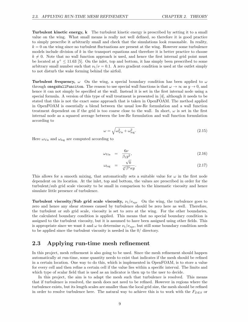
Turbulent kinetic energy, k The turbulent kinetic energy is prescribed by setting it to a smallvalue on the wing. What small means is really not well defined, so therefore it is good practiceto simply prescribe it arbitrarily small and check that the simulations look reasonable. In reality,k = 0 on the wing since no turbulent fluctuations are present at the wing. However some turbulencemodels include division of k in the transport equations and therefore it is better practice to choosek 6= 0. Note that no wall function approach is used, and hence the first internal grid point mustbe located at y+ ≤ 11.63 [5]. On the inlet, top and bottom, it has simply been prescribed to somearbitrary small number such that νt/ν = 0.1. A zero gradient condition is used at the outlet simplyto not disturb the wake forming behind the airfoil.
Turbulent frequency, ω On the wing, a special boundary condition has been applied to ωthrough omegaWallFunciton. The reason to use special wall functions is that ω →∞ as y → 0, andhence it can not simply be specified at the wall. Instead it is set in the first internal node using aspecial formula. A version of this type of wall treatment is presented in [4], although it needs to bestated that this is not the exact same approach that is taken in OpenFOAM. The method appliedin OpenFOAM is essentially a blend between the usual low-Re formulation and a wall functiontreatment dependent on if the grid is too coarse close to the wall. In short, ω is set in the firstinternal node as a squared average between the low-Re formulation and wall function formulationaccording to
ω =√ω2Vis + ω2
log. (2.15)
Here ωVis and ωlog are computed according to
ωVis =6ν
β1y2, (2.16)
ωlog =
√k
4√β∗κy
. (2.17)
This allows for a smooth mixing, that automatically sets a suitable value for ω in the first nodedependent on its location. At the inlet, top and bottom, the values are prescribed in order for theturbulent/sub grid scale viscosity to be small in comparison to the kinematic viscosity and hencesimulate little presence of turbulence.
Turbulent viscosity/Sub grid scale viscosity, νt/νsgs On the wing, the turbulence goes tozero and hence any shear stresses caused by turbulence should be zero here as well. Therefore,the turbulent or sub grid scale, viscosity is set to zero at the wing. For the other boundaries,the calculated boundary condition is applied. This means that no special boundary condition isassigned to the turbulent viscosity, but it is assumed to have been assigned using other fields. Thisis appropriate since we want k and ω to determine νt/νsgs, but still some boundary condition needsto be applied since the turbulent viscosity is needed in the 0/ directory.
2.3 Applying run-time mesh refinement
In this project, mesh refinement is also going to be used. Since the mesh refinement should happenautomatically at run-time, some quantity needs to exist that indicates if the mesh should be refinedin a certain location. One way to do this, which is implemented in OpenFOAM, is to store a valuefor every cell and then refine a certain cell if the value lies within a specific interval. The limits andwhich type of scalar field that is used as an indicator is then up to the user to decide.
In this project, the aim is to adapt the mesh such that turbulence is resolved. This meansthat if turbulence is resolved, the mesh does not need to be refined. However in regions where theturbulence exists, but its length scales are smaller than the local grid size, the mesh should be refinedin order to resolve turbulence here. The natural way to achieve this is to work with the FDES or
9
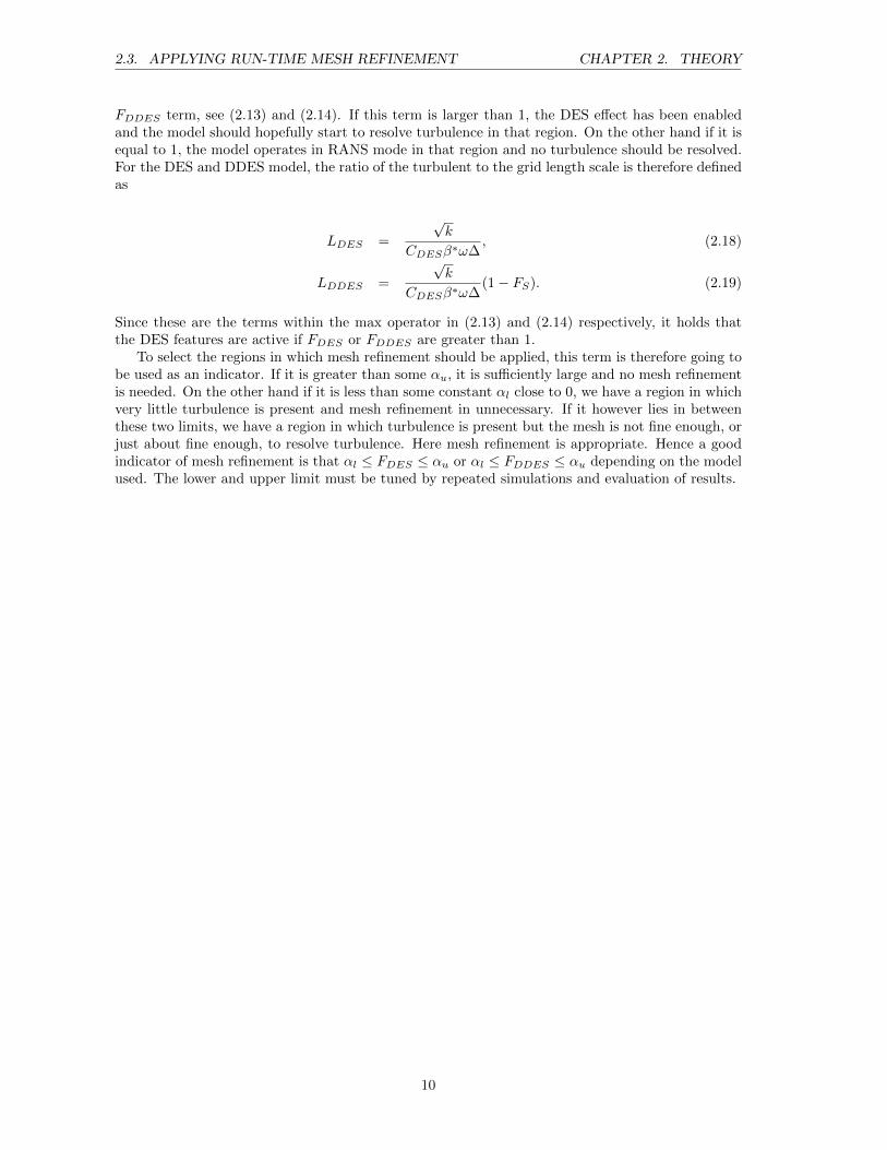
2.3. APPLYING RUN-TIME MESH REFINEMENT CHAPTER 2. THEORY
FDDES term, see (2.13) and (2.14). If this term is larger than 1, the DES effect has been enabledand the model should hopefully start to resolve turbulence in that region. On the other hand if it isequal to 1, the model operates in RANS mode in that region and no turbulence should be resolved.For the DES and DDES model, the ratio of the turbulent to the grid length scale is therefore definedas
LDES =
√k
CDESβ∗ω∆, (2.18)
LDDES =
√k
CDESβ∗ω∆(1− FS). (2.19)
Since these are the terms within the max operator in (2.13) and (2.14) respectively, it holds thatthe DES features are active if FDES or FDDES are greater than 1.
To select the regions in which mesh refinement should be applied, this term is therefore going tobe used as an indicator. If it is greater than some αu, it is sufficiently large and no mesh refinementis needed. On the other hand if it is less than some constant αl close to 0, we have a region in whichvery little turbulence is present and mesh refinement in unnecessary. If it however lies in betweenthese two limits, we have a region in which turbulence is present but the mesh is not fine enough, orjust about fine enough, to resolve turbulence. Here mesh refinement is appropriate. Hence a goodindicator of mesh refinement is that αl ≤ FDES ≤ αu or αl ≤ FDDES ≤ αu depending on the modelused. The lower and upper limit must be tuned by repeated simulations and evaluation of results.
10
Chapter 3
The OpenFOAM implementation
In this chapter the implementation of a LES-class turbulence model, namely the k − ω SST SASmodel, as well as the dynamic mesh features of the pimpleDyMFoam solver are described. The reasonthat the k − ω SST SAS model will be described is that it will later be modified into the k − ωSST DES model as mentioned in the introduction. The discussion does mainly regard high levelprogramming and technical details on a deeper level are left out. The aim is to give a generalunderstanding of the implementation in order to be able to modify the turbulence model as well asusing the dynamic mesh features of the solver.
3.1 k − ω SST SAS model
The declaration and definition files of the k − ω SST SAS turbulence model are found at
$FOAM_SRC/turbulenceModels/incompressible/LES/kOmegaSSTSAS/
3.1.1 kOmegaSSTSAS.H
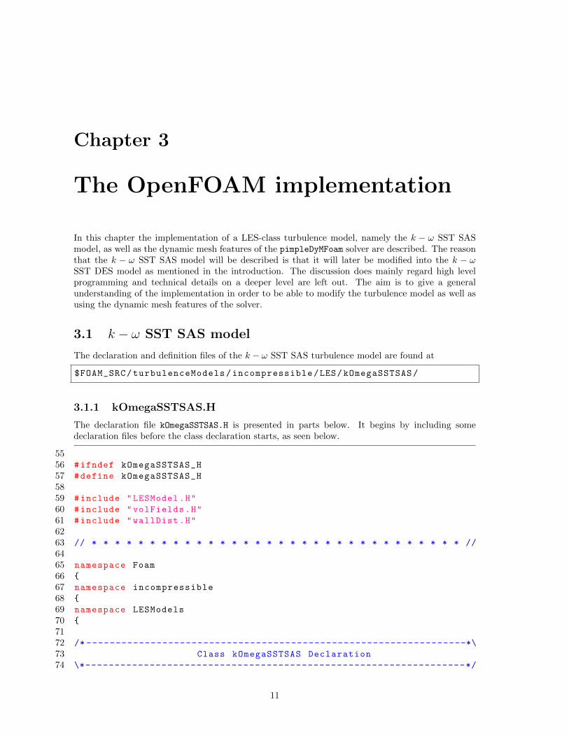
The declaration file kOmegaSSTSAS.H is presented in parts below. It begins by including somedeclaration files before the class declaration starts, as seen below.
5556 #ifndef kOmegaSSTSAS_H
57 #define kOmegaSSTSAS_H
5859 #include "LESModel.H"
60 #include "volFields.H"
61 #include "wallDist.H"
6263 // * * * * * * * * * * * * * * * * * * * * * * * * * * * * * * * * //
6465 namespace Foam
66
67 namespace incompressible
68
69 namespace LESModels
70
7172 /* -----------------------------------------------------------------*\
73 Class kOmegaSSTSAS Declaration
74 \*-----------------------------------------------------------------*/
11
3.1. K − ω SST SAS MODEL CHAPTER 3. THE OPENFOAM IMPLEMENTATION
7576 class kOmegaSSTSAS
77 :
78 public LESModel
79
80 // Private Member Functions
8182 //- Update sub -grid scale fields
83 void updateSubGridScaleFields(const volScalarField& D);
8485 // Disallow default bitwise copy construct and assignment
86 kOmegaSSTSAS(const kOmegaSSTSAS &);
87 kOmegaSSTSAS& operator =( const kOmegaSSTSAS &);
888990 protected:
9192 // Protected data
9394 // Model constants
9596 dimensionedScalar alphaK1_;
97 dimensionedScalar alphaK2_;
9899 dimensionedScalar alphaOmega1_;
100 dimensionedScalar alphaOmega2_;
Listing 3.1: file: kOmegaSSTSAS.H
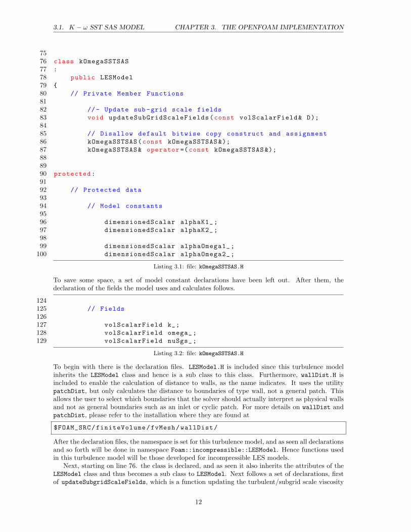
To save some space, a set of model constant declarations have been left out. After them, thedeclaration of the fields the model uses and calculates follows.
124125 // Fields
126127 volScalarField k_;
128 volScalarField omega_;
129 volScalarField nuSgs_;
Listing 3.2: file: kOmegaSSTSAS.H
To begin with there is the declaration files. LESModel.H is included since this turbulence modelinherits the LESModel class and hence is a sub class to this class. Furthermore, wallDist.H isincluded to enable the calculation of distance to walls, as the name indicates. It uses the utilitypatchDist, but only calculates the distance to boundaries of type wall, not a general patch. Thisallows the user to select which boundaries that the solver should actually interpret as physical wallsand not as general boundaries such as an inlet or cyclic patch. For more details on wallDist andpatchDist, please refer to the installation where they are found at
$FOAM_SRC/finiteVolume/fvMesh/wallDist/
After the declaration files, the namespace is set for this turbulence model, and as seen all declarationsand so forth will be done in namespace Foam::incompressible::LESModel. Hence functions usedin this turbulence model will be those developed for incompressible LES models.
Next, starting on line 76. the class is declared, and as seen it also inherits the attributes of theLESModel class and thus becomes a sub class to LESModel. Next follows a set of declarations, firstof updateSubgridScaleFields, which is a function updating the turbulent/subgrid scale viscosity
12
3.1. K − ω SST SAS MODEL CHAPTER 3. THE OPENFOAM IMPLEMENTATION
using call-by-reference. Since it does not say public: or protected: above we also know that thisis a private member function.
After this a set of member constants and member fields are declared. They are set as pro-tected, meaning that they are visible only within this class and classes that inherit from the classkOmegaSSTSAS as well as friend functions to this class. Also when run-time mesh refinement is used,a separate field depicting where mesh refinement should occur is needed as well. For this purposea new volScalarField will have to be added as well. The model constants that the SAS and DESimplementation share have the same values in both models. The only difference is that the modelsuse some specific constants in their respective source terms. It should also be mentioned that thenames used in this implementation differ to some extent from the names found in [2]. When describ-ing how to do the DES implementation, the corresponding names in literature and implementationwill be presented to avoid confusion.
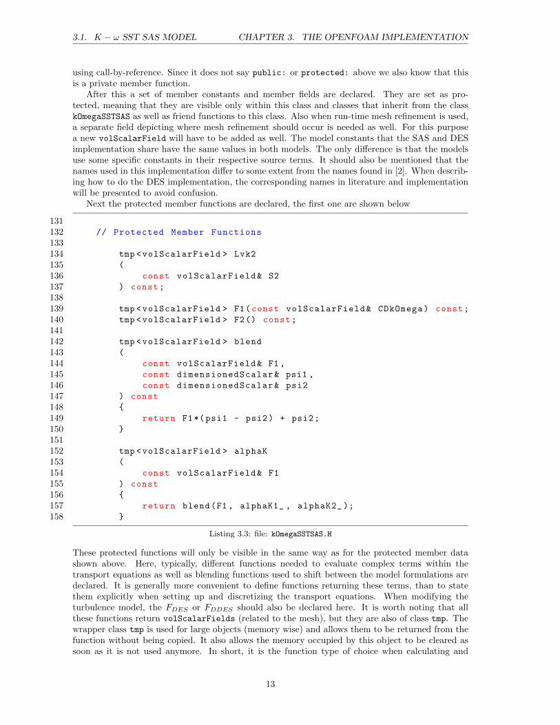
Next the protected member functions are declared, the first one are shown below
131132 // Protected Member Functions
133134 tmp <volScalarField > Lvk2
135 (
136 const volScalarField& S2
137 ) const;
138139 tmp <volScalarField > F1(const volScalarField& CDkOmega) const;
140 tmp <volScalarField > F2() const;
141142 tmp <volScalarField > blend
143 (
144 const volScalarField& F1 ,
145 const dimensionedScalar& psi1 ,
146 const dimensionedScalar& psi2
147 ) const
148
149 return F1*(psi1 - psi2) + psi2;
150
151152 tmp <volScalarField > alphaK
153 (
154 const volScalarField& F1
155 ) const
156
157 return blend(F1, alphaK1_ , alphaK2_ );
158
Listing 3.3: file: kOmegaSSTSAS.H
These protected functions will only be visible in the same way as for the protected member datashown above. Here, typically, different functions needed to evaluate complex terms within thetransport equations as well as blending functions used to shift between the model formulations aredeclared. It is generally more convenient to define functions returning these terms, than to statethem explicitly when setting up and discretizing the transport equations. When modifying theturbulence model, the FDES or FDDES should also be declared here. It is worth noting that allthese functions return volScalarFields (related to the mesh), but they are also of class tmp. Thewrapper class tmp is used for large objects (memory wise) and allows them to be returned from thefunction without being copied. It also allows the memory occupied by this object to be cleared assoon as it is not used anymore. In short, it is the function type of choice when calculating and
13
3.1. K − ω SST SAS MODEL CHAPTER 3. THE OPENFOAM IMPLEMENTATION
returning large fields that will only be used temporarily to compute some term or quantity in thetransport equations. Furthermore, the keyword const is predominantly used throughout memberfunction declarations above. The second const, used after defining which parameters to take in,says that this function may not modify the original objects it takes in. The first ones says that theobject sent in is of type constant.
The function blend is also defined here, not just declared. It is the implementation of (2.7) and(2.8) and is used to blend the model constants. The reason to why only one type of blend functionis needed is that the values of 1/σkj and 1/σωj are used instead of σkj and σωj . An example of howblend is applied is seen in the next member function, where 1/σk is computed using the blendingbetween the k − ω and the k − ε values. As can be seen the model constants do not have the samename in the implementation as in the papers it is based upon.
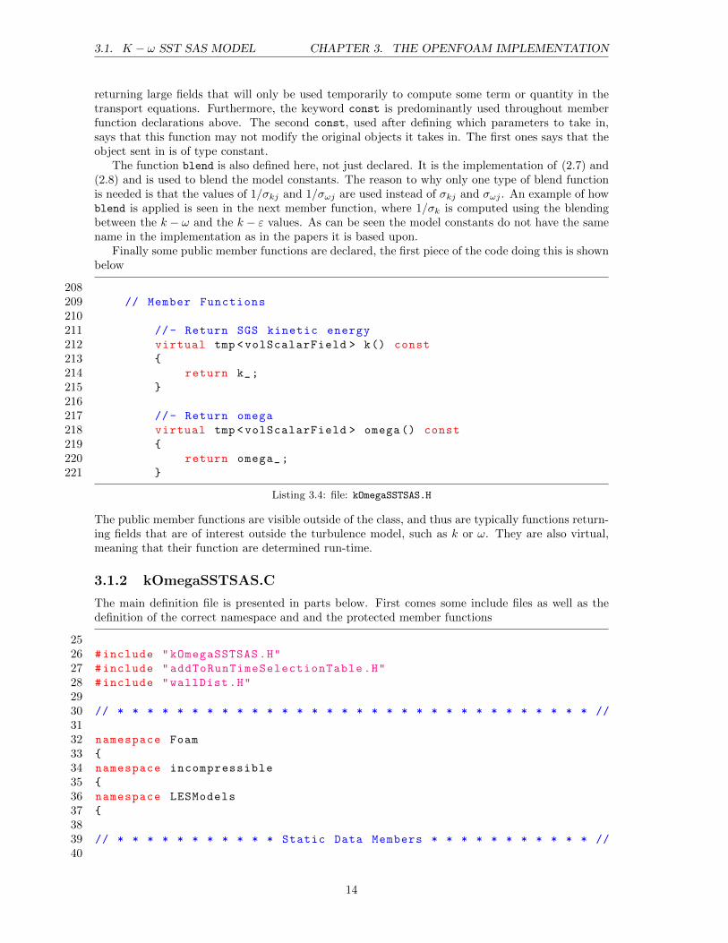
Finally some public member functions are declared, the first piece of the code doing this is shownbelow
208209 // Member Functions
210211 //- Return SGS kinetic energy
212 virtual tmp <volScalarField > k() const
213
214 return k_;
215
216217 //- Return omega
218 virtual tmp <volScalarField > omega() const
219
220 return omega_;
221
Listing 3.4: file: kOmegaSSTSAS.H
The public member functions are visible outside of the class, and thus are typically functions return-ing fields that are of interest outside the turbulence model, such as k or ω. They are also virtual,meaning that their function are determined run-time.
3.1.2 kOmegaSSTSAS.C
The main definition file is presented in parts below. First comes some include files as well as thedefinition of the correct namespace and and the protected member functions
2526 #include "kOmegaSSTSAS.H"
27 #include "addToRunTimeSelectionTable.H"
28 #include "wallDist.H"
2930 // * * * * * * * * * * * * * * * * * * * * * * * * * * * * * * * * //
3132 namespace Foam
33
34 namespace incompressible
35
36 namespace LESModels
37
3839 // * * * * * * * * * * * Static Data Members * * * * * * * * * * * //
40
14
3.1. K − ω SST SAS MODEL CHAPTER 3. THE OPENFOAM IMPLEMENTATION
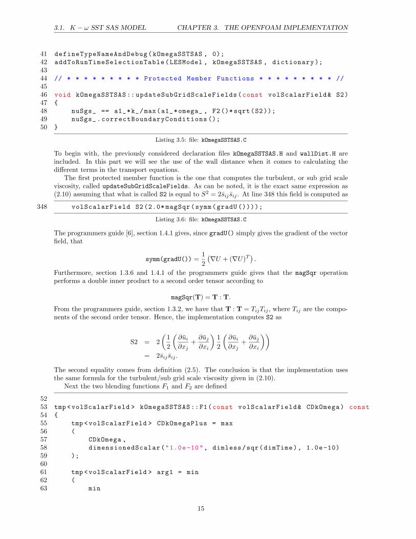
41 defineTypeNameAndDebug(kOmegaSSTSAS , 0);
42 addToRunTimeSelectionTable(LESModel , kOmegaSSTSAS , dictionary );
4344 // * * * * * * * * * Protected Member Functions * * * * * * * * * //
4546 void kOmegaSSTSAS :: updateSubGridScaleFields(const volScalarField& S2)
47
48 nuSgs_ == a1_*k_/max(a1_*omega_ , F2()* sqrt(S2));
49 nuSgs_.correctBoundaryConditions ();
50
Listing 3.5: file: kOmegaSSTSAS.C
To begin with, the previously considered declaration files kOmegaSSTSAS.H and wallDist.H areincluded. In this part we will see the use of the wall distance when it comes to calculating thedifferent terms in the transport equations.
The first protected member function is the one that computes the turbulent, or sub grid scaleviscosity, called updateSubGridScaleFields. As can be noted, it is the exact same expression as(2.10) assuming that what is called S2 is equal to S2 = 2sij sij . At line 348 this field is computed as
348 volScalarField S2 (2.0* magSqr(symm(gradU ())));
Listing 3.6: file: kOmegaSSTSAS.C
The programmers guide [6], section 1.4.1 gives, since gradU() simply gives the gradient of the vectorfield, that
symm(gradU()) =1
2
(∇U + (∇U)T
).
Furthermore, section 1.3.6 and 1.4.1 of the programmers guide gives that the magSqr operationperforms a double inner product to a second order tensor according to
magSqr(T) = T : T.
From the programmers guide, section 1.3.2, we have that T : T = TijTij , where Tij are the compo-nents of the second order tensor. Hence, the implementation computes S2 as
S2 = 2
(1
2
(∂ui∂xj
+∂uj∂xi
)1
2
(∂ui∂xj
+∂uj∂xi
))= 2sij sij .
The second equality comes from definition (2.5). The conclusion is that the implementation usesthe same formula for the turbulent/sub grid scale viscosity given in (2.10).
Next the two blending functions F1 and F2 are defined
5253 tmp <volScalarField > kOmegaSSTSAS ::F1(const volScalarField& CDkOmega) const
54
55 tmp <volScalarField > CDkOmegaPlus = max
56 (
57 CDkOmega ,
58 dimensionedScalar("1.0e-10", dimless/sqr(dimTime), 1.0e-10)
59 );
6061 tmp <volScalarField > arg1 = min
62 (
63 min
15
3.1. K − ω SST SAS MODEL CHAPTER 3. THE OPENFOAM IMPLEMENTATION
64 (
65 max
66 (
67 (scalar (1)/ betaStar_ )*sqrt(k_)/( omega_*y_),
68 scalar (500)* nu()/( sqr(y_)* omega_)
69 ),
70 (4* alphaOmega2_ )*k_/( CDkOmegaPlus*sqr(y_))
71 ),
72 scalar (10)
73 );
7475 return tanh(pow4(arg1 ));
76
777879 tmp <volScalarField > kOmegaSSTSAS ::F2() const
80
81 tmp <volScalarField > arg2 = min
82 (
83 max
84 (
85 (scalar (2)/ betaStar_ )*sqrt(k_)/( omega_*y_),
86 scalar (500)* nu()/( sqr(y_)* omega_)
87 ),
88 scalar (100)
89 );
9091 return tanh(sqr(arg2 ));
92
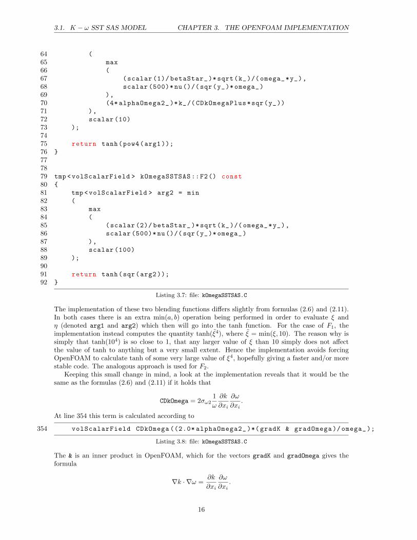
Listing 3.7: file: kOmegaSSTSAS.C
The implementation of these two blending functions differs slightly from formulas (2.6) and (2.11).In both cases there is an extra min(a, b) operation being performed in order to evaluate ξ andη (denoted arg1 and arg2) which then will go into the tanh function. For the case of F1, theimplementation instead computes the quantity tanh(ξ4), where ξ = min(ξ, 10). The reason why issimply that tanh(104) is so close to 1, that any larger value of ξ than 10 simply does not affectthe value of tanh to anything but a very small extent. Hence the implementation avoids forcingOpenFOAM to calculate tanh of some very large value of ξ4, hopefully giving a faster and/or morestable code. The analogous approach is used for F2.
Keeping this small change in mind, a look at the implementation reveals that it would be thesame as the formulas (2.6) and (2.11) if it holds that
CDkOmega = 2σω21
ω
∂k
∂xi
∂ω
∂xi.
At line 354 this term is calculated according to
354 volScalarField CDkOmega ((2.0* alphaOmega2_ )*( gradK & gradOmega )/ omega_ );
Listing 3.8: file: kOmegaSSTSAS.C
The & is an inner product in OpenFOAM, which for the vectors gradK and gradOmega gives theformula
∇k · ∇ω =∂k
∂xi
∂ω
∂xi.
16
3.1. K − ω SST SAS MODEL CHAPTER 3. THE OPENFOAM IMPLEMENTATION
Hence the implementation uses the desired formula for the cross diffusion term as given in (2.9).The rest of the implemented protected member functions are specific to the SAS model. When
adding the new FDES or FDDES term later on, it will be convenient to include it as a function likeF1. This will make it easy to modify and view its implementation as well as switching between theDES and DDES formulation. Later on a volScalarField can then be created using this function,prior to setting up and solving the discrete system of equations.
Next comes the construction of the object kOmegaSSTSAS
116117 // * * * * * * * * * * * * * Constructors * * * * * * * * * * * * //
118119 kOmegaSSTSAS :: kOmegaSSTSAS
120 (
121 const volVectorField& U,
122 const surfaceScalarField& phi ,
123 transportModel& transport ,
124 const word& turbulenceModelName ,
125 const word& modelName
126 )
127 :
128 LESModel(modelName , U, phi , transport , turbulenceModelName),
129130 alphaK1_
131 (
132 dimensioned <scalar >:: lookupOrAddToDict
133 (
134 "alphaK1",
135 coeffDict_ ,
136 0.85034
137 )
138 ),
139 alphaK2_
140 (
141 dimensioned <scalar >:: lookupOrAddToDict
142 (
143 "alphaK2",
144 coeffDict_ ,
145 1.0
146 )
147 ),
Listing 3.9: file: kOmegaSSTSAS.C
To save some space, not all definitions of protected member constants have been included. They arefollowed by the fields used by the turbulence model as follows.
286287 k_
288 (
289 IOobject
290 (
291 "k",
292 runTime_.timeName(),
293 mesh_ ,
294 IOobject ::MUST_READ ,
295 IOobject :: AUTO_WRITE
17
3.1. K − ω SST SAS MODEL CHAPTER 3. THE OPENFOAM IMPLEMENTATION
296 ),
297 mesh_
298 ),
299300 omega_
301 (
302 IOobject
303 (
304 "omega",
305 runTime_.timeName(),
306 mesh_ ,
307 IOobject ::MUST_READ ,
308 IOobject :: AUTO_WRITE
309 ),
310 mesh_
311 ),
312313 nuSgs_
314 (
315 IOobject
316 (
317 "nuSgs",
318 runTime_.timeName(),
319 mesh_ ,
320 IOobject ::MUST_READ ,
321 IOobject :: AUTO_WRITE
322 ),
323 mesh_
324 )
325
326 omegaMin_.readIfPresent (*this);
327328 bound(k_, kMin_ );
329 bound(omega_ , omegaMin_ );
330331 updateSubGridScaleFields (2.0* magSqr(symm(fvc::grad(U))));
332333 printCoeffs ();
334
Listing 3.10: file: kOmegaSSTSAS.C
After the appropriate parameters have been taken in to construct the object kOmegaSSTSAS, the con-struction begins by directly calling the constructor of the LESModel class. After this all model con-stants are read from a sub dictionary in the LESProperties dictionary called kOmegaSSTSASCoeffs,or defined if not present. Also all the relevant fields, such as k and ω are read. Since the DESmodel includes a new model constant, it is important to include it here as well. Also, in the case ofrun-time mesh refinement, a new field is needed which will be computed by the turbulence model.Thus it must also be read here in order to be computed. The maybe most important thing in thebody of the constructor is the call for the calculation of the turbulent viscosity through the functionupdateSubGridScaleFields.
The final part of the turbulence model includes solving for the turbulent quantities k and ω to-gether with the calculation of νt/νsgs. This is done in the virtual void function correct, whichis a public member function of the class kOmegaSSTSAS as can be seen in the declaration filekOmegaSSTSAS.H. Hence, since it is a virtual function, it will override the function correct in
18
3.1. K − ω SST SAS MODEL CHAPTER 3. THE OPENFOAM IMPLEMENTATION
the LESModel class, which the kOmegaSSTSAS class inherited. This allows OpenFOAM to selectwhich turbulence model that is used run-time, since the function calculating the turbulent viscosityis overridden by the chosen turbulence model. It starts by solving the equation for k
336337 // * * * * * * * * * * * * Member Functions * * * * * * * * * * * //
338339 void kOmegaSSTSAS :: correct(const tmp <volTensorField >& gradU)
340
341 LESModel :: correct(gradU );
342343 if (mesh_.changing ())
344
345 y_.correct ();
346
347348 volScalarField S2 (2.0* magSqr(symm(gradU ())));
349 gradU.clear ();
350351 volVectorField gradK(fvc::grad(k_));
352 volVectorField gradOmega(fvc::grad(omega_ ));
353 volScalarField L(sqrt(k_)/( pow025(Cmu_)* omega_ ));
354 volScalarField CDkOmega ((2.0* alphaOmega2_ )*( gradK & gradOmega )/ omega_ );
355 volScalarField F1(this ->F1(CDkOmega ));
356 volScalarField G(GName(), nuSgs_*S2);
357358 // Turbulent kinetic energy equation
359
360 fvScalarMatrix kEqn
361 (
362 fvm::ddt(k_)
363 + fvm::div(phi(), k_)
364 - fvm:: laplacian(DkEff(F1), k_)
365 ==
366 min(G, c1_*betaStar_*k_*omega_)
367 - fvm::Sp(betaStar_*omega_ , k_)
368 );
369370 kEqn.relax ();
371 kEqn.solve ();
372
373 bound(k_, kMin_ );
374375 tmp <volScalarField > grad_omega_k = max
376 (
377 magSqr(gradOmega )/sqr(omega_),
378 magSqr(gradK )/sqr(k_)
379 );
Listing 3.11: file: kOmegaSSTSAS.C
What can first be noted is that support for a changing mesh is included, in which case the walldistance will be corrected by letting the function correct() operate on the field. After this a setof fields necessary to set up the discrete system of equations are calculated. Since the names ofthe different operations are very logical in OpenFOAM, it is not necessary to explain all of these
19
3.1. K − ω SST SAS MODEL CHAPTER 3. THE OPENFOAM IMPLEMENTATION
fields. The fields S2 and CDkOmega have already been considered, and the only one that raises somequestions is the field called G. This is the production term Pk without the limiter applied to it, sinceaccording to the implementation we have
G = νtS2
= νt2sij sij
= 2νtsij(sij + Ωij
)= νt
(∂ui∂xj
+uj∂xi
)[1
2
(∂ui∂xj
+∂uj∂xi
)+
1
2
(∂ui∂xj− ∂uj∂xi
)]= νt
(∂ui∂xj
+uj∂xi
)∂ui∂xj
= Pk.
Here it was used that the product of the anti symmetric tensor Ωij and the symmetric tensor sij iszero since Ωij = −Ωji.
When implementing the DES model it is the dissipation in the k equation that will be modifiedby multiplying it with an extra term, namely FDES or FDDES . This field must also be calculatedin advance using the function describing it.
Turning to the creation of the discrete system of equations, the transport equation for k is setup in accordance with (2.2) apart from the fact that no DES term is included. The production termcan be seen to include the limiter, as written in (2.12) since c1 = 10. Further the dissipation termcomes in by using the operation fvm::Sp(betaStar *omega , k ). Indeed the dissipation termcould simply have been added by writing betaStar *omega *k , in which case it would have beenimplemented explicitly. The thing is though that the entire dissipation term always is negative dueto the minus sign, and the fact that k, ω and β∗ are positive. To improve convergence and stabilityit is better to treat negative sources implicitly, which is achieved using the syntax Sp(). The answerto why is because when a source term is treated explicitly, it is included in the load vector b in thediscretisized system of equations Ak = b, where k is a vector including the nodal values of k. Henceit can prior to convergence cause the elements in k to go negative, which is bad when consideringthat k ≥ 0 by definition. However, when it is treated implicitly, it is instead included in the diagonalof A instead. Since it was negative on the right hand side, it will instead give a positive contributionon the left hand side, making the matrix A more diagonally dominant.
After the k equation has been solved, the ω equation is set up and solved according to
380381 // Turbulent frequency equation
382
383 fvScalarMatrix omegaEqn
384 (
385 fvm::ddt(omega_)
386 + fvm::div(phi(), omega_)
387 - fvm:: laplacian(DomegaEff(F1), omega_)
388 ==
389 gamma(F1)*S2
390 - fvm::Sp(beta(F1)*omega_ , omega_)
391 - fvm::SuSp // cross diffusion term
392 (
393 (F1 - scalar (1))* CDkOmega/omega_ ,
394 omega_
395 )
396 + FSAS_
397 *max
398 (
20
3.2. PIMPLEDYMFOAM CHAPTER 3. THE OPENFOAM IMPLEMENTATION
399 dimensionedScalar("zero",dimensionSet (0, 0, -2, 0, 0), 0.0),
400 zetaTilda2_*kappa_*S2*sqr(L/Lvk2(S2))
401 - 2.0/ alphaPhi_*k_*grad_omega_k
402 )
403 );
404405 omegaEqn.relax ();
406 omegaEqn.solve ();
407
408 bound(omega_ , omegaMin_ );
409410 updateSubGridScaleFields(S2);
411
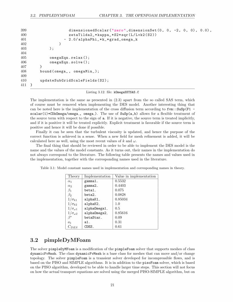
Listing 3.12: file: kOmegaSSTSAS.C
The implementation is the same as presented in (2.3) apart from the so called SAS term, whichof course must be removed when implementing the DES model. Another interesting thing thatcan be noted here is the implementation of the cross diffusion term according to fvm::SuSp(F1 -
scalar(1)*CDkOmega/omega , omega ). The use of SuSp(a,b) allows for a flexible treatment ofthe source term with respect to the sign of a. If it is negative, the source term is treated implicitly,and if it is positive it will be treated explicitly. Explicit treatment is favorable if the source term ispositive and hence it will be done if possible.
Finally it can be seen that the turbulent viscosity is updated, and hence the purpose of thecorrect function is achieved in a sense. When a new field for mesh refinement is added, it will becalculated here as well, using the most recent values of k and ω.
The final thing that should be reviewed in order to be able to implement the DES model is thename and the values of the model constants. As it turns out, their names in the implementation donot always correspond to the literature. The following table presents the names and values used inthe implementation, together with the corresponding names used in the literature.
Table 3.1: Model constant names used in implementation and corresponding names in theory.
Theory Implementation Value in implementationα1 gamma1 0.5532α2 gamma2 0.4403β1 beta1 0.075β2 beta2 0.08281/σk1 alphaK1 0.850341/σk2 alphaK2 1.01/σω1 alphaOmega1 0.51/σω2 alphaOmega2 0.85616β∗ betaStar 0.09a1 a1 0.31CDES CDES 0.61
3.2 pimpleDyMFoam
The solver pimpleDyMFoam is a modification of the pimpleFoam solver that supports meshes of classdynamicFvMesh. The class dynamicFvMesh is a base class for meshes that can move and/or changetopology. The solver pimpleFoam is a transient solver developed for incompressible flows, and isbased on the PISO and SIMPLE algorithms. It is in addition to the pisoFoam solver, which is basedon the PISO algorithm, developed to be able to handle larger time steps. This section will not focuson how the actual transport equations are solved using the merged PISO-SIMPLE algorithm, but on
21
3.2. PIMPLEDYMFOAM CHAPTER 3. THE OPENFOAM IMPLEMENTATION
how the dynamic meshes are treated within the solver. There are a number of different sub classesto the class dynamicFvMesh, based upon what the mesh should be able to do. Since pimpleDyMFoam
primarily is developed for moving meshes, special attention will also be paid towards how this solverwill treat a refined mesh and if there are missing features left to be implemented for this purpose.The pimpleDyMFoam solver is located at
$FOAM_APP/applications/solvers/incompressible/pimpleFoam /\
pimpleDyMFoam/
Furthermore, for reference, the pimpleFoam solver are located at
$FOAM_APP/applications/solvers/incompressible/pimpleFoam/
3.2.1 Comparison between pimpleFoam.C and pimpleDyMFoam.C
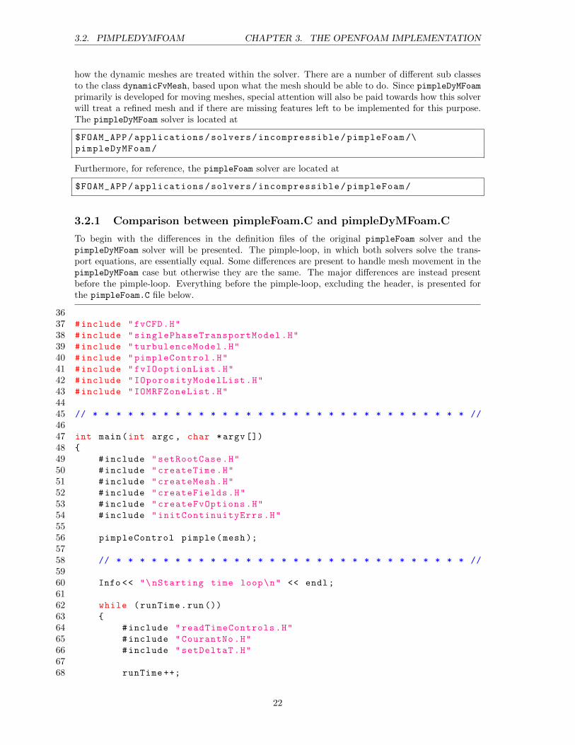
To begin with the differences in the definition files of the original pimpleFoam solver and thepimpleDyMFoam solver will be presented. The pimple-loop, in which both solvers solve the trans-port equations, are essentially equal. Some differences are present to handle mesh movement in thepimpleDyMFoam case but otherwise they are the same. The major differences are instead presentbefore the pimple-loop. Everything before the pimple-loop, excluding the header, is presented forthe pimpleFoam.C file below.
3637 #include "fvCFD.H"
38 #include "singlePhaseTransportModel.H"
39 #include "turbulenceModel.H"
40 #include "pimpleControl.H"
41 #include "fvIOoptionList.H"
42 #include "IOporosityModelList.H"
43 #include "IOMRFZoneList.H"
4445 // * * * * * * * * * * * * * * * * * * * * * * * * * * * * * * * * //
4647 int main(int argc , char *argv [])
48
49 #include "setRootCase.H"
50 #include "createTime.H"
51 #include "createMesh.H"
52 #include "createFields.H"
53 #include "createFvOptions.H"
54 #include "initContinuityErrs.H"
5556 pimpleControl pimple(mesh);
5758 // * * * * * * * * * * * * * * * * * * * * * * * * * * * * * * //
5960 Info << "\nStarting time loop\n" << endl;
6162 while (runTime.run())
63
64 #include "readTimeControls.H"
65 #include "CourantNo.H"
66 #include "setDeltaT.H"
6768 runTime ++;
22
3.2. PIMPLEDYMFOAM CHAPTER 3. THE OPENFOAM IMPLEMENTATION
6970 Info << "Time = " << runTime.timeName () << nl << endl;
Listing 3.13: file: pimpleFoam.C
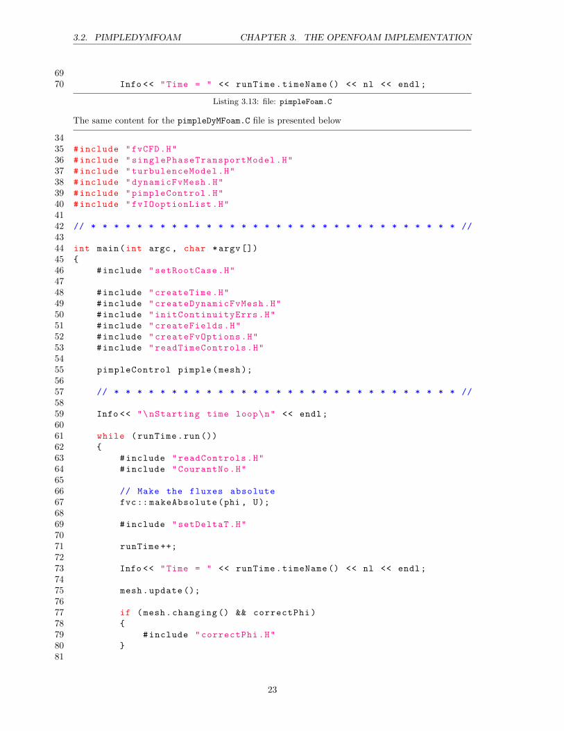
The same content for the pimpleDyMFoam.C file is presented below
3435 #include "fvCFD.H"
36 #include "singlePhaseTransportModel.H"
37 #include "turbulenceModel.H"
38 #include "dynamicFvMesh.H"
39 #include "pimpleControl.H"
40 #include "fvIOoptionList.H"
4142 // * * * * * * * * * * * * * * * * * * * * * * * * * * * * * * * * //
4344 int main(int argc , char *argv [])
45
46 #include "setRootCase.H"
4748 #include "createTime.H"
49 #include "createDynamicFvMesh.H"
50 #include "initContinuityErrs.H"
51 #include "createFields.H"
52 #include "createFvOptions.H"
53 #include "readTimeControls.H"
5455 pimpleControl pimple(mesh);
5657 // * * * * * * * * * * * * * * * * * * * * * * * * * * * * * * //
5859 Info << "\nStarting time loop\n" << endl;
6061 while (runTime.run())
62
63 #include "readControls.H"
64 #include "CourantNo.H"
6566 // Make the fluxes absolute
67 fvc:: makeAbsolute(phi , U);
6869 #include "setDeltaT.H"
7071 runTime ++;
7273 Info << "Time = " << runTime.timeName () << nl << endl;
7475 mesh.update ();
7677 if (mesh.changing () && correctPhi)
78
79 #include "correctPhi.H"
80
81
23
3.2. PIMPLEDYMFOAM CHAPTER 3. THE OPENFOAM IMPLEMENTATION
82 // Make the fluxes relative to the mesh motion
83 fvc:: makeRelative(phi , U);
8485 if (mesh.changing () && checkMeshCourantNo)
86
87 #include "meshCourantNo.H"
88
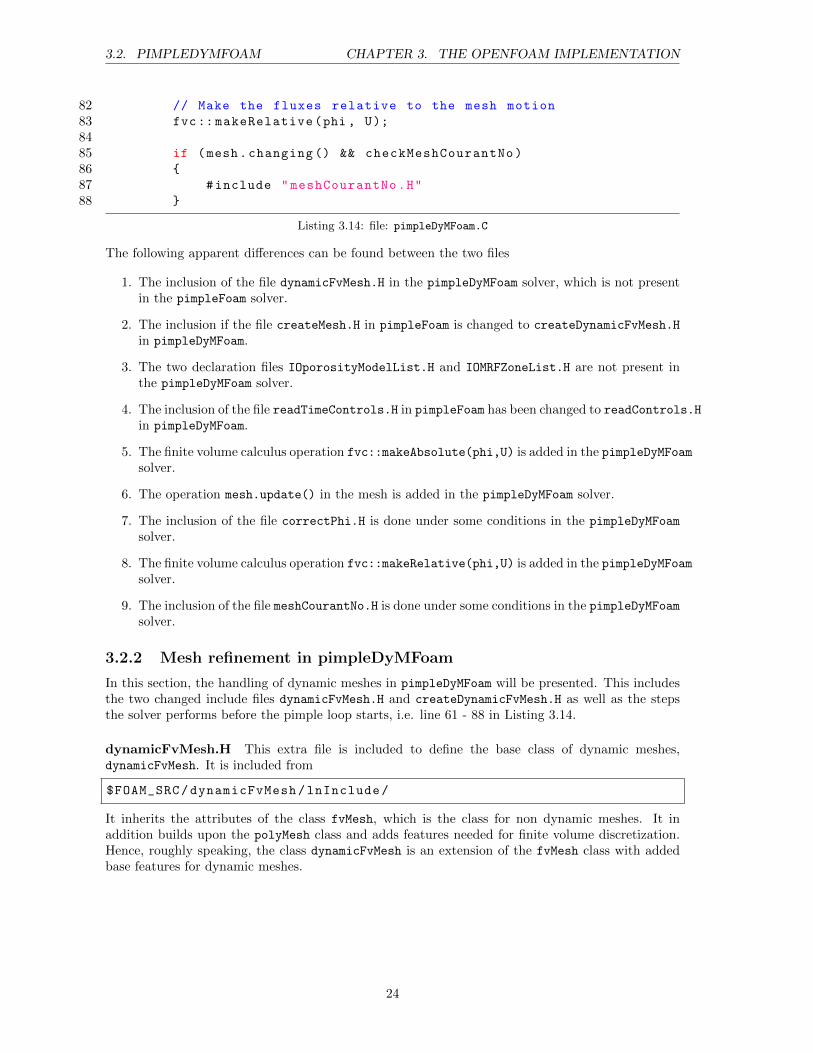
Listing 3.14: file: pimpleDyMFoam.C
The following apparent differences can be found between the two files
1. The inclusion of the file dynamicFvMesh.H in the pimpleDyMFoam solver, which is not presentin the pimpleFoam solver.
2. The inclusion if the file createMesh.H in pimpleFoam is changed to createDynamicFvMesh.H
in pimpleDyMFoam.
3. The two declaration files IOporosityModelList.H and IOMRFZoneList.H are not present inthe pimpleDyMFoam solver.
4. The inclusion of the file readTimeControls.H in pimpleFoam has been changed to readControls.Hin pimpleDyMFoam.
5. The finite volume calculus operation fvc::makeAbsolute(phi,U) is added in the pimpleDyMFoamsolver.
6. The operation mesh.update() in the mesh is added in the pimpleDyMFoam solver.
7. The inclusion of the file correctPhi.H is done under some conditions in the pimpleDyMFoam
solver.
8. The finite volume calculus operation fvc::makeRelative(phi,U) is added in the pimpleDyMFoamsolver.
9. The inclusion of the file meshCourantNo.H is done under some conditions in the pimpleDyMFoamsolver.
3.2.2 Mesh refinement in pimpleDyMFoam
In this section, the handling of dynamic meshes in pimpleDyMFoam will be presented. This includesthe two changed include files dynamicFvMesh.H and createDynamicFvMesh.H as well as the stepsthe solver performs before the pimple loop starts, i.e. line 61 - 88 in Listing 3.14.
dynamicFvMesh.H This extra file is included to define the base class of dynamic meshes,dynamicFvMesh. It is included from
$FOAM_SRC/dynamicFvMesh/lnInclude/
It inherits the attributes of the class fvMesh, which is the class for non dynamic meshes. It inaddition builds upon the polyMesh class and adds features needed for finite volume discretization.Hence, roughly speaking, the class dynamicFvMesh is an extension of the fvMesh class with addedbase features for dynamic meshes.
24
3.2. PIMPLEDYMFOAM CHAPTER 3. THE OPENFOAM IMPLEMENTATION
createDynamicFvMesh.H This file is used as a substitute to the createFvMesh.H file. It is alsoincluded from
$FOAM_SRC/dynamicFvMesh/lnInclude/
What it does is that it uses a function in the file dynamicFvMeshNew.C, located in the same directory,to create a mesh of the class specified in the dynamicMeshDict dictionary, located in the constantdirectory of the case. In the case of mesh refinement, this class will be called dynamicRefineFvMesh,for which refinement specific functions are defined.
readControls.H This file is included instead of the file readTimeControls.H and is located inthe same directory as the solver. It is an extension of this file and reads
1 #include "readTimeControls.H"
23 const dictionary& pimpleDict = pimple.dict ();
45 const bool correctPhi =
6 pimpleDict.lookupOrDefault("correctPhi", false );
78 const bool checkMeshCourantNo =
9 pimpleDict.lookupOrDefault("checkMeshCourantNo", false );
1011 const bool ddtPhiCorr =
12 pimpleDict.lookupOrDefault("ddtPhiCorr", true);
Listing 3.15: file: readControls.H
The file readTimeControls.H is located at
$FOAM_SRC/finiteVolume/cfdTools/general/include/
It is used to look up time parameters in the controlDict dictionary, located in the system directoryof the case. The first one is the boolean variable adjustTimeStep, which is set to false by default.The second one is the scalar maxCo which is used to specify the maximum Courant number and isset to 1 by default. The last one is the scalar maxDeltaT, used to specify the largest allowed timestep in the simulation, and it is set to a large value by default.
For the purpose of dynamic meshes, the readControls.H file also includes three new booleanvariables, namely correctPhi, checkMeshCourantNo and ddtPhiCorr. These variables are set inthe fvSolution dictionary, within the section specifying the PIMPLE controls. The specific use ofthese variables will be discussed when they are used later in the code.
CourantNo.H This file is located at
$FOAM_SRC/finiteVolume/cfdTools/incompressible/
It is used to calculate and print out the mean and max Courant number based on the previously usedtime step. In case the time step is taken as constant, i.e. adjustTimeStep = false, the Courantnumber calculation only serves to inform the user of which Courant number the time step and meshgives. The Courant number is furthermore computed in OpenFOAM according to
Co =1
2
∑f |φf |∆V
∆t.
Here, φf = Af (nf · uf ), is the velocity flux normal to surface f of the mesh control volume withvolume ∆V . For a hexahedral mesh with straight edges, this formula will give the following formulafor the Courant number
25
3.2. PIMPLEDYMFOAM CHAPTER 3. THE OPENFOAM IMPLEMENTATION
Co =
(|ux|∆x
+|uy|∆y
+|uz|∆z
)∆t.
This is a common form to express the Courant number, which according to the Courant-Friedrichs-Lewy condition generally should be less than 1 to obtain stable solutions to time marching problems.
fvc::makeAbsolute(phi, U) This function is defined in the file fvcMeshPhi.C that is located at
$FOAM_SRC/finiteVolume/lnInclude/
This operation adds the flux caused by the movement of the mesh to the flux across the mesh controlvolume boundaries. This gives the absolute flux relative to a fixed and non moving boundary, insteadof the flux relative to the movement of the mesh control volume boundaries. This operation willalso only be performed in the case where the mesh is moving, and hence for mesh refinement it willnot be used.
setDeltaT.H This file is also found in
$FOAM_SRC/finiteVolume/lnInclude/
This routine sets the value for ∆t to be used in the next time integration. It does this to satisfy theconditions that the maximum Courant number as well as time step, if specified in the controlDict,are not exceeded. It does this using the Courant number calculated recently, which is based on thecurrent velocities and previous time step. Also note that in the case of a moving mesh, the fact thatthe fluxes have been made absolute already does not affect this routine since the Courant number wasevaluated prior to the makeAbsolute routine was called. Denoting the maximum Courant numberand time step set in the controlDict by maxCo and maxDeltaT, the calculated Courant numberCoNum, and the previous time step ∆t, the current time step, ∆t, is according to the implementationcalculated as
∆F =maxCo
CoNum,
∆F = min(min(∆F, 1 + 0.1∆F ), 1.2),
∆t = min(∆F∆t, maxDeltaT).
Hence, the new value ∆t is set based on the old value ∆t multiplied with a scaling factor ∆F . Thesecond equation serves to relax this scaling factor in order to avoid too large increases in time stepsand thereby unstable solutions. If the relaxation does not become active, the algorithm calculates ∆tas the largest possible time step allowed, either by the Courant number condition or the maximumtime step condition. Finally this routines prints out the new time step.
mesh.update() The function update() operates on the mesh depending on which subclass todynamicFvMesh that it belongs to. In case of mesh refinement, this class is called dynamicRefineFvMesh,and the corresponding implementation of update() is found in the file dynamicRefineFvMesh.C lo-cated at
$FOAM_SRC/dynamicFvMesh/dynamicRefineFvMesh/
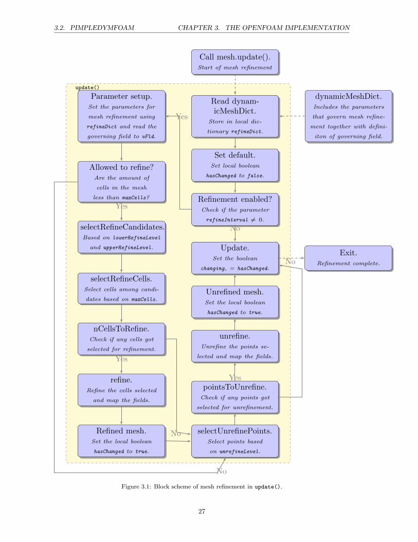
The function update() itself starts at line 1073 and in Figure 3.1 a simplified block scheme of thefunction is presented.
26
3.2. PIMPLEDYMFOAM CHAPTER 3. THE OPENFOAM IMPLEMENTATION
update()
Call mesh.update().Start of mesh refinement
Read dynam-icMeshDict.
Store in local dic-
tionary refineDict.
dynamicMeshDict.Includes the parameters
that govern mesh refine-
ment together with defini-
iton of governing field.
Set default.Set local boolean
hasChanged to false.
Refinement enabled?Check if the parameter
refineInterval 6= 0.
Parameter setup.Set the parameters for
mesh refinement using
refineDict and read the
governing field to vFld.
Allowed to refine?Are the amount of
cells in the mesh
less than maxCells?
selectRefineCandidates.Based on lowerRefineLevel
and upperRefineLevel.
selectRefineCells.Select cells among candi-
dates based on maxCells.
nCellsToRefine.Check if any cells got
selected for refinement.
refine.Refine the cells selected
and map the fields.
Refined mesh.Set the local boolean
hasChanged to true.
selectUnrefinePoints.Select points based
on unrefineLevel.
pointsToUnrefine.Check if any points got
selected for unrefinement.
unrefine.Unrefine the points se-
lected and map the fields.
Unrefined mesh.Set the local boolean
hasChanged to true.
Update.Set the boolean
changing = hasChanged.
Exit.Refinement complete.
Yes
Yes
Yes
No
Yes
No
No
No
Figure 3.1: Block scheme of mesh refinement in update().
27
3.2. PIMPLEDYMFOAM CHAPTER 3. THE OPENFOAM IMPLEMENTATION
To begin with, it reads the dictionary dynamicMeshDict (Read dynamicMeshDict), located inthe constant directory of the case. This dictionary specifies all the parameters that will govern themesh refinement together with the name of the field that the refinement will be based on. Thedictionary is stored in the local dictionary called refineDict.
The function uses a local boolean variable called hasChanged, which will be true if the mesh hasbeen refined or unrefined. To begin with, no modifications to the mesh has been done and hence itis set to false by default (Set default).
After this the function will check if refinement is enabled or not (Refinement enabled?). Thismeans that the parameter refineInterval in refineDict is checked. If this parameter is set to0, the function will not enable mesh refinement, but instead go to Update. This enables the userto run pimpleDyMFoam without refinement, which can be useful if a converged solution is desiredbefore enabling mesh refinement. If the parameter refineInterval is greater than 0, the functionwill enable mesh refinement/unrefinement with time step intervals specified by the parameter. Inthis case it will move on (Parameter setup).
The next step is simply to extract all parameters from the refineDict and create local variables(Parameter setup). In addition to this, the field that govern mesh refinement is read as well andput into the local field vFld. The field governs mesh refinement in the sense that it’s values in everycell are used to determine if that cell should be refined/unrefined or not as we will see soon.
To avoid the mesh refinement to create too many cells, which could cause the memory or compu-tational time to explode, there is a parameter maxCells specifying the maximum amount of cells themesh may include. The function will therefore check the current amount of cells against maxCells
before refining the mesh and creating more cells (Allowed to refine?). If the amount of cells aregreater than nCells, the function will proceed to the unrefinement (selectUnrefine).
In case there is room for refinement, the function will proceed to select candidate cells forrefinement (selectRefineCandidates). A cell will become a candidate if the value of vFld in celli lies in between the defined limits, i.e.
lowerRefineLevel < vFldi < upperRefineLevel.
This checking is done in the local function error, which computes the error of each cell i, defined as
erri = min(vFldi − lowerRefineLevel, upperRefineLevel− vFldi).
If erri ≥ 0 for a given cell, then that cell will be marked as a candidate for refinement. It is nothard to see that this calculation gives the criteria that the field value should lie within the specifiedlimits. For a qualified cell, the value erri represent the closest distance to either of the limitslowerRefineLevel or upperRefineLevel. This information is not used later on, but comments inthe code suggest that it is intended to be used in later versions to do a better selection of cells torefine. For now however, a cell is either a candidate or not.
When the candidates for refinement have been selected, it is time to proceed and select the cellsthat will actually be refined among these candidates (selectRefineCells). There are two cases
Table 3.2: Parameters that can be set in the dynamicMeshDict.
Parameter Description Allowed valuesrefineInterval Amount of time steps between refinement 0 ≤maxRefinement Maximum cellLevel for a cell that is refined 0 ≤maxCells Maximum amount of cells in mesh allowed 0 <field Name of field that govern refinement/unrefinement ”field name”lowerRefineLevel Lower limit of field value in a cell to allow refinement 0 <upperRefineLevel Upper limit of field value in a cell to allow refinement 0 <unrefineLevel Upper limit value of field value in a cell to allow unrefinement ≤ 0uBufferLayers Amount of buffer layers for unrefinement < 0correctFluxes List of fluxes to be remapped on newly created faces List of namesdumpLevel Unknown boolean variable true/false
28
3.2. PIMPLEDYMFOAM CHAPTER 3. THE OPENFOAM IMPLEMENTATION
that can emerge at this stage. In the first case, the number of cells after refinement of all thecandidate cells will not exceed maxCells. In the second case, the amount of cells after refinement ofall candidates cells would exceed maxCells, which is not allowed. To estimate the amount of cellsafter refinement, the function assumes that every refined cell is split into 8 new ones. This meansthat for every refined cell, the total amount of cells will increase by 7. Hence, the total amount ofcells that can be refined, nTotToRefine, can be estimated as
nTotToRefine =maxCells - nTotCells
7,
where nTotCells is used to denote the total amount of cells prior to refinement. Based on thisestimation, the code then decides which of the two cases described above that exist. If the amountof candidates are less than nTotToRefine, we have the first case and vice versa if the amount ofcandidates are more. In the first case, the code allows, or marks, all candidates for refinement. Inthe second case it will simply select cells for refinement until the total amount becomes larger thannTotToRefine. Hence no intelligent selection is performed in this implementation, but as far as theauthor understands it, the foundation for better selection has been laid.
At this stage the function has a set of cells that will be refined and that satisfies all the listedcriteria above. Before moving on to the refinement routine, the function will also do a trivial checkto see if any cells got selected for refinement at all (nCellsToRefine). It could be the case that nocell was selected since the value of the field vFld did not match for any cell. If this is the case thefunction will move on to the unrefinement procedure.
In the case where cells got selected, the cells will be refined and the fields will be mappedonto the new mesh. This all happens in the routine called refine, which starts at line 205 indynamicRefineFvMesh.C. The details of how the mapping is performed and how the mesh is splithave not been investigated in any detail. The code however claims that the fields are mapped andthat a new approximate flux is calculated at the newly created faces. This correction/mapping willonly be done if the fluxes have been listed under correctFluxes in the dynamicMeshDict. Pleasenote that many time integration algorithms, such as backward Euler or Crank Nicholson, use oldvalues, not only those of the current time step, to integrate to the next time step. This means thatcorrectFluxes needs to include these as well. How this is done will be shown in the tutorial later.If the fluxes are not recreated the function will still work and solver run, but the results will beredundant.
After refinement and mapping has been performed, the function will set the local booleanhasChanged to true (Refined mesh). It will then move on to the unrefinement.
The next thing that happens is that the function will select points to unrefine (selectUnrefinePoints).Of course, a cell in itself can not be unrefined, but rather a common corner of a set of cells canbe removed to create a larger cell. The selection of points to remove is made among those corre-sponding to cells that have not been refined. In fact, the function also allows for the possibility toprotect neighboring cells to cells that have been refined from being unrefined. This is possible tocontrol through the parameter nBufferLayers in the dynamicMeshDict. This allows the user tospecify how many layers of cells from those that have been refined that should be protected fromunrefinement. The restoring points will now be selected for unrefinement based on the criteria thatthe (interpolated) value of the field vFld at point i satisfies
pFldi < unrefineLevel.
The interpolation is done by taking the average value of the field vFld in the neighboring cells.Before moving on to the mesh unrefinement, the function also checks if any points got selected
for unrefinement (pointsToUnrefine).If it turned out that some points qualified for unrefinement, the mesh will be unrefined using
the routine unrefine. As before, the fields are also mapped and the fluxes are recreated approxi-mately on the new faces. Also as before, the fluxes will only be recreated if they are listed undercorrectFluxes in the dynamicMeshDict.
Since the mesh has changed, the local boolean hasChanged will be set to true (Unrefined mesh).This is done since it may happen that the mesh only was unrefined.
29
3.2. PIMPLEDYMFOAM CHAPTER 3. THE OPENFOAM IMPLEMENTATION
The function concludes in the step that have been named Update here. In this step a functioncalled changing is called with the boolean hasChanged as parameter. This function belongs tothe class polyMesh, which all dynamicFvMesh classes are subclasses of. This function changes theboolean changing in the polyMesh class to the value of the parameter supplied to the function.This boolean can thus be used, as will be seen later, to see if the mesh was changed this time stepor not.
correctPhi.H This routine is located in the same directory as the solver, i.e. it is written specif-ically for this solver. As seen from Listing 3.14, it is only going to be active if the two booleansmesh.changing() and correctPhi are true. The second one we have already seen, it is set inthe fvSolution dictionary and read by readControls.H. Hence, the user chooses whenever thisroutine will take effect or not, since the boolean correctPhi is set to false by default. The firstboolean is returned from the member function changing(), whose definition can be found in thefile polyMesh.H included from
$FOAM_SRC/OpenFOAM/lnInclude/
This file declares the class polyMesh, which is inherited by the class fvMesh, which in addition isinherited by the dynamicFvMesh class and its sub classes. The definition of the public memberfunction changing() furthermore reads
468469 //- Is mesh changing (topology changing and/or moving)
470 bool changing () const
471
472 return changing_;
473
Listing 3.16: file: polyMesh.H
Hence, this function returns the boolean changing , which was set to true if the mesh is refined, asnoted previously.
In the file correctPhi.H, the pressure corrector equation of the PIMPLE algorithm is solved forthe amount of times prescribed by the variable nNonOrthogonalCorrectors, set in the fvSolution
dictionary. The part of the code that does this reads
5354 while (pimple.correctNonOrthogonal ())
55
56 fvScalarMatrix pcorrEqn
57 (
58 fvm:: laplacian(rAU , pcorr) == fvc::div(phi)
59 );
6061 pcorrEqn.setReference(pRefCell , pRefValue );
62 pcorrEqn.solve ();
6364 if (pimple.finalNonOrthogonalIter ())
65
66 phi -= pcorrEqn.flux ();
67
68
Listing 3.17: file: correctPhi.H
The purpose of this is to obtain a so called pressure corrector that will be used to correct the fluxesover the mesh cells to obey continuity. The reason to why this is included prior to actually entering
30
3.2. PIMPLEDYMFOAM CHAPTER 3. THE OPENFOAM IMPLEMENTATION
the PIMPLE loop further down the code is to compensate for the fact that the mesh may havechanged. In a case where the mesh changes, the different fields need to be mapped from the oldto the new mesh. This will naturally introduce some interpolation error, which for the case of facefluxes, can cause continuity to not be obeyed anymore on the new mesh. Hence, this part of thecode offers the possibility to correct the fluxes to obey continuity before solving for the next timestep. Speaking generally, when solving numerically for the next time step, the current time stepcomes in as a source term in the linear system of equations that is solved for. Therefore, since anerror has been introduced in the mapping between the meshes, this error will continue to affect thesolution in the next time step. Note that this argument is valid for any field that is solved for, i.e.not only the velocity field.
fvc::makeRelative(phi, U) This routine performs the opposite operation of fvc::makeAbsolute(phi,U). It’s defined in the file fvcMeshPhi.C found in
$FOAM_SRC/finiteVolume/lnInclude/
This function hence subtracts the flux of the mesh at every cell face, leaving the flux at the cellfaces that is relative to the moving mesh. Since this routine only is used in cases where the mesh ismoving, it is not used when mesh refinement is.
meshCourantNo.H The file meshCourantNo.H is included from
$FOAM_SRC/dynamicFvMesh/lnInclude/
As can be noted from Listing 3.14, this routine is used in the case where the mesh has changed(mesh.changing()) and if the boolean checkMeshCourantNo has been set to true. The secondboolean we saw was set in readControls.H, where it was read from the fvSolution dictionary.The routine in meshCourantNo.H performs the exact same operations as the routine found inCourantNo.H considered previously but for the flux caused by the mesh. In other words, the fluxover the cell faces caused by the mesh motion is used instead of the relative flux of the fluid overthe cell faces. This means that the mesh Courant number is based on the velocity of the meshrather than the fluid. It’s use has not been further investigated, since the mesh is not moving in therefinement case and thus this routine should not be used.
3.2.3 Suggested modifications for mesh refinement
The pimpleDyMFoam solver is mainly developed to handle moving meshes but can also handle meshrefinement. Since it is originally written for moving meshes, there are some features that are missingand that in some way should be implemented in the future to obtain a better solver.
Smoother for turbulent quantities As noted when considering the include file correctPhi.H,the fluxes are corrected in order to satisfy continuity over the computational cells. This addressesthe problem introduced by mapping the velocity/flux field but not the fact that turbulent quantitiessuch as k, ε or ω have been mapped as well. As discussed before, the solution at the current timestep affects the solution of the next time step and hence if the current solution have obtained a largeerror in the mapping procedure, this error will live on to the next time step. It is therefore suggestedthat a ”smoothing” procedure is introduced after the velocity field has been corrected but beforethe PIMPLE loop start. This would constitute of a set of iterations in the solution of the turbulentequations in order to converge the solution of the turbulent quantities on the new mesh.
Adjusting ∆t for the new mesh In cases where the Courant number is used to limit the valueof ∆t, it was noted above that this is done prior to updating the mesh. This means that the valueof ∆t is based on the Courant number obtained on the mesh prior to mesh refinement. If the meshwould be refined, come cells are split into smaller cells. In the current case, ∆t, as well as thevelocities ux, uy and uz are fixed. According to the definition of the Courant number, this would
31

3.2. PIMPLEDYMFOAM CHAPTER 3. THE OPENFOAM IMPLEMENTATION
mean that if for example ∆x, ∆y and ∆z are divided by two, the Courant number for those cellswould become twice as large. Hence, the way the solver operates right now will cause the actualCourant number to becomes larger in refined cells, which may cause instabilities. The solution wouldbe to incorporate a recalculation of the Courant number after mesh refinement, as well updating ∆tbased on this. These routines should naturally only be active in the case of mesh refinement and beincluded after the velocity field/fluxes have been corrected. Note also that the update of the timethrough runTime++ would have to be moved as well.
32
Chapter 4
Implementing k − ω SST DES
The first section of this chapter describes step by step how the turbulence model k−ω SST DES canbe obtained by modifying the existing k − ω SST SAS model. The next section then describes howto further modify the turbulence model to produce a volScalarField that can control the meshrefinement.
4.1 k − ω SST DES
In this section a new source term in the k equation will be added, which which is a modification ofthe dissipation. Terms unique to the SAS model will also be taken away to avoid unnecessary termor constants being computed.
One thing that is important in order to achieve the correct turbulence model is to make sure thatthe different terms in the transport equations that are reused actually are implemented as describedin the paper. This is due to that turbulence models often get modified over the years even thoughthe actual name stays the same. This was done in a previous section, and this analysis will be thebasis for the step by step guide below in how to implement the k − ω SST DES turbulence model.
4.1.1 Copying the kOmegaSSTSAS model
To begin with, the SAS model will be copied into the user directory. Start by opening a new terminalwindow and type
OF22x
to initialize the OpenFOAM 2.2.x environment. Next change directory to
cd $WM_PROJECT_DIR
Now copy the kOmegaSSTSAS turbulence model into the user directory according to
cp -r --parents src/turbulenceModels/incompressible/LES/\
kOmegaSSTSAS/ $WM_PROJECT_USER_DIR
Finally change directory to where the turbulence model has been copied in the user directory ac-cording to
cd $WM_PROJECT_USER_DIR/src/turbulenceModels/incompressible/LES/
4.1.2 Creating the class kOmegaSSTDES
To create a new class, start by changing name of the directory according to
33
4.1. K − ω SST DES CHAPTER 4. IMPLEMENTING K − ω SST DES
mv kOmegaSSTSAS/ kOmegaSSTDES/
Now continue by removing the .dep file inside the turbulence model directory and change name ofthe .C and .H file to an appropriate name
rm kOmegaSSTDES/kOmegaSSTSAS.dep
mv kOmegaSSTDES/kOmegaSSTSAS.C kOmegaSSTDES/kOmegaSSTDES.C
mv kOmegaSSTDES/kOmegaSSTSAS.H kOmegaSSTDES/kOmegaSSTDES.H
Now we need a Make directory where the make files will reside, it should lie in the same directoryas the turbulence model directory. Create it and then go into it according to
mkdir Make/
cd Make/
Now we will create the necessary files files and options. Starting with files, it may be createdas
gedit files
In the new empty file, we must add our new turbulence model to tell the compiler creating thedynamic turbulence model library where the new turbulence model should be included. Do this byincluding the lines
kOmegaSSTDES/kOmegaSSTDES.C
LIB = $(FOAM_USER_LIBBIN )/ libmyIncompressibleLESModels
The content of files is similar to the one found in the installation. The difference is that thelibrary should be put in $(FOAM USER LIBBIN) instead and the name should be changed from beinglibIncompressibleLESModels to something else.
Next the options file is created according to
gedit options
In the new file that opens, add the following lines
EXE_INC = \
-I$(LIB_SRC )/ turbulenceModels \
-I$(LIB_SRC )/ turbulenceModels/LES/LESdeltas/lnInclude \
-I$(LIB_SRC )/ turbulenceModels/LES/LESfilters/lnInclude \
-I$(LIB_SRC )/ transportModels \
-I$(LIB_SRC )/ finiteVolume/lnInclude \
-I$(LIB_SRC )/ meshTools/lnInclude \
-I$(LIB_SRC )/ turbulenceModels/incompressible/LES/lnInclude
LIB_LIBS =
These lines are also found in the original options file in the installation except for the last includeline. This one is needed since the turbulence model does not lie in the original directory anymore,but still needs files from there.
Now change directory to where the declaration and definition files are located
cd ../ kOmegaSSTDES/
To change the name of the class, we must substitute the line ”kOmegaSSTSAS” to ”kOmegaSST-DES” in both the declaration file and the definition file. This is done according to
34
4.1. K − ω SST DES CHAPTER 4. IMPLEMENTING K − ω SST DES
sed -i s/kOmegaSSTSAS/kOmegaSSTDES/g kOmegaSSTDES.H
sed -i s/kOmegaSSTSAS/kOmegaSSTDES/g kOmegaSSTDES.C
A good practice is to also look through the files and make sure that the name of the class haschanged. Finish by first cleaning up the turbulence model library and then compile the turbulencemodel in order to see that everything works so far
cd ..
wclean
wmake libso
4.1.3 Modifying kOmegaSSTDES.H
We will start by modifying the file kOmegaSSTDES.H, so begin by changing directory and open it
cd $WM_PROJECT_USER_DIR/src/turbulenceModels/incompressible/LES/\
kOmegaSSTDES/
gedit kOmegaSSTDES.H
The reader may of course choose another editor instead of gedit. We will start by adding a newheader to our new file, so that it is clear which turbulence model we actually use, do this by changingthe lines
Description
kOmegaSSTDES LES turbulence model for incompressible flows
based on:
"Evaluation of the SST -SAS model: channel flow , asymmetric diffuser
and axi -symmetric hill".
European Conference on Computational Fluid Dynamics ECCOMAS CFD 2006.
Lars Davidson
The first term of the Qsas expression is corrected following:
DESider A European Effort on Hybrid RANS -LES Modelling:
Results of the European -Union Funded Project , 2004 - 2007
(Notes on Numerical Fluid Mechanics and Multidisciplinary Design ).
Chapter 2, section 8 Formulation of the Scale -Adaptive Simulation (SAS)
Model during the DESIDER Project. Published in Springer -Verlag Berlin
Heidelberg 2009.
F. R. Menter and Y. Egorov.
Listing 4.1: file: kOmegaSSTDES.H
to the following new description, including a small disclaimer
Description
k-Omega -SST -DES LES turbulence model for incompressible flows
based on:
"Ten Years of Industrial Experience with the SST Turbulence Model".
Turbulence Heat and Mass Transfer 4.
F. R. Menter , M. Kuntz , R. Langtry.
35
4.1. K − ω SST DES CHAPTER 4. IMPLEMENTING K − ω SST DES
A note on the implementation with respect to the paper:
- The transport equations implemented are divided by rho , as opposed to the
presentation of them in the paper , since the flow is incompressible
- There is a choice to use the model in DES (Detached Eddy Simulation) mode
or DDES (Delayed Detached Eddy Simulations) mode. The latter protects the
boundary layer from being resolved with LES and is used by default. The
other part is commented away.
- Model constants are not allways named the same as in the paper , see comments
in declaration of constants below.
-------------------------------------------------------------------------------
DISCLAIMER:
This is a student project work in the course CFD with OpenSource software
taught by Hakan Nilsson , Chalmers University of Technology , Gothenburg , Sweden.
-------------------------------------------------------------------------------
Listing 4.2: file: kOmegaSSTDES.H
Now lets comment away unnecessary model constants that are unique to the SAS model. Start bycommenting away the following lines
dimensionedScalar Cs_;
dimensionedScalar alphaPhi_;
dimensionedScalar zetaTilda2_;
dimensionedScalar FSAS_;
Listing 4.3: file: kOmegaSSTDES.H
to obtain
// dimensionedScalar Cs_;
// dimensionedScalar alphaPhi_;
// dimensionedScalar zetaTilda2_;
// dimensionedScalar FSAS_;
Listing 4.4: file: kOmegaSSTDES.H
After this, comment away the last two SAS model constants and also add the new constant CDESas a dimensionedScalar. Do this by modifying the lines
dimensionedScalar Cmu_;
dimensionedScalar kappa_;
Listing 4.5: file: kOmegaSSTDES.H
to
// dimensionedScalar Cmu_;
// dimensionedScalar kappa_;
dimensionedScalar CDES_; // C_DES
Listing 4.6: file: kOmegaSSTDES.H
36
4.1. K − ω SST DES CHAPTER 4. IMPLEMENTING K − ω SST DES
Now the new model includes the correct model constants in the class declaration. If the reader wantsto, it can also add a comment after each model constant, like it has been done for CDES , with thename of the constant in the paper. For a reference to these names please see Table 3.1.
The next thing to do is to comment away the protected member function called Lvk2. This is afunction exclusive to the SAS model which computes the Von Karman length scale used to identifyunsteadiness and trigger LES mode in the SAS model. After commenting, the code should read
/*
tmp <volScalarField > Lvk2
(
const volScalarField& S2
) const;
*/
Listing 4.7: file: kOmegaSSTDES.H
As noted earlier when studying the SAS implementation, it is convenient to use a function thatcreates the FDES or FDDES term. To give the user a choice, both terms will be added, but one ofthem will be commented away and hence not become active when compiling the dynamic library.As Menter implies that the DDES implementation with the boundary layer protector is the safestapproach, it will be the one applied in this case [1]. Therefore add the following lines after thedeclaration of the blend function
// Choose DES or DDES by commenting the non desired option
// tmp <volScalarField > FDES() const;
tmp <volScalarField > FDDES(const volScalarField& FS) const;
Listing 4.8: file: kOmegaSSTDES.H
If the reader would like to use DES model instead, it is merely a matter of switching the commentingor simply adding only the term preferred. As seen, the function is returning a volScalarField oftype tmp, which is the preferred alternative when defining function that will be evaluated for everycell in the mesh and thus return large amount of data. As can be seen as well, the FDDES termtakes in the argument FS, which as stated in the theory can be chosen as either F1 or F2.
After this step the necessary changes to the kOmegaSSTDES.H file are done, next is the filekOmegaSSTDES.C.
4.1.4 Modifying kOmegaSSTDES.C
As seen previously, the definition file starts with defining the protected member functions. The firstthing that therefore needs to be done is to remove the definition of the Von Karman length scale,Lvk2. Hence comment away its definition to obtain
/*
tmp <volScalarField > kOmegaSSTDES ::Lvk2
(
const volScalarField& S2
) const
return max
(
kappa_*sqrt(S2)
37
4.1. K − ω SST DES CHAPTER 4. IMPLEMENTING K − ω SST DES
/(
mag(fvc:: laplacian(U()))
+ dimensionedScalar
(
"ROOTVSMALL",
dimensionSet (0, -1 , -1, 0, 0, 0, 0),
ROOTVSMALL
)
),
Cs_*delta()
);
*/
Listing 4.9: file: kOmegaSSTDES.C
With this done, its time to define the FDES and FDDES terms. In this implementation, the DDESterm is used and hence the other term should be commented away. This is achieved by adding thefollowing lines directly after the Lvk2 just commented away
// Choose DES or DDES by commenting the non desired option
// F_DES term definition
/*
tmp <volScalarField > kOmegaSSTDES ::FDES() const
return max
(
sqrt(k_)/( CDES_*betaStar_*omega_*delta()),
scalar (1)
);
*/
// F_DDES term definition , FS = F1 or F2 may be chosen as the
// boundary layer protector
tmp <volScalarField > kOmegaSSTDES :: FDDES(const volScalarField& FS) const
return max
(
sqrt(k_)/( CDES_*betaStar_*omega_*delta ())*( scalar (1) - FS),
scalar (1)
);
Listing 4.10: file: kOmegaSSTDES.C
Next in the code comes the constructor of the class kOmegaSSTDES, and here we need to include ournew model constant CDES as well as remove constants no longer in use. The constants that shouldbe removed are Cs , alphaPhi , zetaTilda2 , FSAS , Cmu and kappa since they are all exclusiveto the SAS model. Make sure to comment away them all, which for Cs simply gives
/*
Cs_
(
dimensioned <scalar >:: lookupOrAddToDict
38
4.1. K − ω SST DES CHAPTER 4. IMPLEMENTING K − ω SST DES
(
"Cs",
coeffDict_ ,
0.262
)
),
*/
Listing 4.11: file: kOmegaSSTDES.C
After all SAS model constants have been commented away, the CDES constant must be defined aswell. Therefore, after the commented constant kappa , add the following lines
CDES_
(
dimensioned <scalar >:: lookupOrAddToDict
(
"CDES",
coeffDict_ ,
0.61
)
),
Listing 4.12: file: kOmegaSSTDES.C
With this accomplished, its time to add the DES functionality in the function correct, which is theone that solves the transport equations and updates the turbulent/sub grid scale viscosity. As theSAS features are also to be removed, these terms will be commented away. To begin with, the fieldsnot used in the model should not be calculated prior to setting up and solving the discrete systemof equations. Therefore comment away the calculation of the field denoted L according to
// volScalarField L(sqrt(k_)/( pow025(Cmu_)* omega_ ));
Listing 4.13: file: kOmegaSSTDES.C
Next its time to calculate the field FDES or FDDES using the previously defined functions. Thisis done by adding the following lines after the production term G has been calculated and prior tosolving for k according to
// volScalarField FDES(this ->FDES ());
volScalarField FDDES(this ->FDDES(F1));
Listing 4.14: file: kOmegaSSTDES.C
Once again, note that it is the DDES features that are implemented here. Also note that it iscrucial that the FDDES is computed after the F1 field, since it relies on it as a parameter. Nextthe transport equation for k is going to be modified so that the dissipation term includes the DESmodification. This is done by adding the newly computed field FDES or FDDES into the first slot ofthe Sp( , ) function creating the source term. The final result should look like
// Turbulent kinetic energy equation
fvScalarMatrix kEqn
(
fvm::ddt(k_)
+ fvm::div(phi(), k_)
39
4.1. K − ω SST DES CHAPTER 4. IMPLEMENTING K − ω SST DES
- fvm:: laplacian(DkEff(F1), k_)
==
min(G, c1_*betaStar_*k_*omega_)
- fvm::Sp(betaStar_*FDDES*omega_ , k_) // F_DDES modification
// - fvm::Sp(betaStar_*FDES*omega_ , k_) // F_DES modification
);
Listing 4.15: file: kOmegaSSTDES.C
Note that it does not work to include the FDES/FDDES term in the second slot, i.e. multiplying itwith k .
After the k equation has been solved, a field unique to the SAS implementation is being calculatedwhich is needed in a source term in the ω equation that is not used in the DES model. This field iscalled grad omega k and should be commented away according to
/*
tmp <volScalarField > grad_omega_k = max
(
magSqr(gradOmega )/sqr(omega_),
magSqr(gradK )/sqr(k_)
);
*/
Listing 4.16: file: kOmegaSSTDES.C
The next thing that needs to be done is to remove the source term in the ω equation that is uniqueto the SAS model. It is the last entity of the equation and should be commented away to get thefollowing
// Turbulent frequency equation
fvScalarMatrix omegaEqn
(
fvm::ddt(omega_)
+ fvm::div(phi(), omega_)
- fvm:: laplacian(DomegaEff(F1), omega_)
==
gamma(F1)*S2
- fvm::Sp(beta(F1)*omega_ , omega_)
- fvm::SuSp // cross diffusion term
(
(F1 - scalar (1))* CDkOmega/omega_ ,
omega_
)
/*
+ FSAS_
*max
(
dimensionedScalar ("zero",dimensionSet (0, 0, -2, 0, 0), 0.0),
zetaTilda2_*kappa_*S2*sqr(L/Lvk2(S2))
- 2.0/ alphaPhi_*k_*grad_omega_k
)
*/
);
40
4.2. K − ω SST DES REFINE CHAPTER 4. IMPLEMENTING K − ω SST DES
Listing 4.17: file: kOmegaSSTDES.C
Finally, the read() function should be modified in order to exclude SAS model constants and includethe new DES model constant. The read() function is present at the end of the file and should bemodified according to
bool kOmegaSSTDES ::read()
if (LESModel ::read ())
alphaK1_.readIfPresent(coeffDict ());
alphaK2_.readIfPresent(coeffDict ());
alphaOmega1_.readIfPresent(coeffDict ());
alphaOmega2_.readIfPresent(coeffDict ());
gamma1_.readIfPresent(coeffDict ());
gamma2_.readIfPresent(coeffDict ());
beta1_.readIfPresent(coeffDict ());
beta2_.readIfPresent(coeffDict ());
betaStar_.readIfPresent(coeffDict ());
a1_.readIfPresent(coeffDict ());
c1_.readIfPresent(coeffDict ());
// Cs_.readIfPresent(coeffDict ());
// alphaPhi_.readIfPresent(coeffDict ());
// zetaTilda2_.readIfPresent(coeffDict ());
// FSAS_.readIfPresent(coeffDict ());
CDES_.readIfPresent(coeffDict ());
omegaMin_.readIfPresent (*this);
return true;
else
return false;
Listing 4.18: file: kOmegaSSTDES.C
This concludes the modification of the turbulence model. The final thing to be done is to removethe kOmegaSSTDES.dep file and then recompile (wclean and then wmake libso). Therefore save andclose the editor and then move into the directory where the Make and kOmegaSSTDES directories aresituated. Then simply type
wclean
wmake libso
This should build a new dynamic library including the new turbulence model. It will then be possibleto link to this library and run simulations using the new turbulence model.
4.2 k − ω SST DES Refine
This section shows how to modify the k − ω SST DES turbulence model implemented above towork with the dynamic mesh refinement features of OpenFOAM. As previously discussed, the mesh
41
4.2. K − ω SST DES REFINE CHAPTER 4. IMPLEMENTING K − ω SST DES
refinement needs a field to determine where the mesh should be refined and not. This field shouldbe located in the time directory and hence must be computed, either by defining a function in theturbulence model or in the solver. This field will be a part of the FDES term of the turbulencemodel and hence the creation and output of this field is what is going to be added to the turbulencemodel.
Before doing this, it should be stressed that the method shown here most certainly is not theonly way to achieve this. The way it will be done is pretty straight forward, and follows the way theturbulent/sub grid scale viscosity is being computed and sent back. It was determined to not usethe new field to further compute the FDES term, even though it is a part of it. Instead this part ofthe FDES term will be recomputed and returned, only to be used to govern mesh refinement. Thereare two reasons for this. The first is that the term includes the mesh size ∆, which only is definedin the node of a cell. Hence, at the boundary, there is no definition of what ∆ should be and hencean appropriate boundary condition can be hard to derive. Since the term will reside in the timedirectory, some boundary conditions should be imposed and thus the solution would run the risk ofbeing affected by these if this term was actually used to evaluate FDES/FDDES . Secondly, it wasfound more convenient to leave the previous implementation intact and just add new features.
4.2.1 Creating the class kOmegaSSTDESRefine
This entire guide assumes that the k−ω SST DES turbulence model already has been implementedaccording to above. Start by opening a new terminal window and type
OF22x
to initialize the OpenFOAM environment. Next change directory to where the user turbulencemodels are implemented
cd $WM_PROJECT_USER_DIR/src/turbulenceModels/incompressible/LES/
Copy the kOmegaSSTDES turbulence model directory into a new directory called kOmegaSST-DESRefine according to
cp -r kOmegaSSTDES/ kOmegaSSTDESRefine/
Change directory to the new turbulence model, remove the old kOmegaSSTDES.dep file and changename of the two remaining files according to
cd kOmegaSSTDESRefine/
rm kOmegaSSTDES.dep
mv kOmegaSSTDES.C kOmegaSSTDESRefine.C
mv kOmegaSSTDES.H kOmegaSSTDESRefine.H
Then substitute the line kOmegaSSTDES for kOmegaSSTDESRefine in both the files, which will changethe name of the class.
sed -i s/kOmegaSSTDES/kOmegaSSTDESRefine/g kOmegaSSTDESRefine.H
sed -i s/kOmegaSSTDES/kOmegaSSTDESRefine/g kOmegaSSTDESRefine.C
Finally the model will be added to the files file, in order to tell the compiler that a new turbulencemodel should be added to the dynamic library. Open it using for example gedit
cd ..
gedit Make/files
and add the following line after the previous turbulence model
kOmegaSSTDESRefine/kOmegaSSTDESRefine.C
Finally recompile the dynamic library and make sure that everything works
42
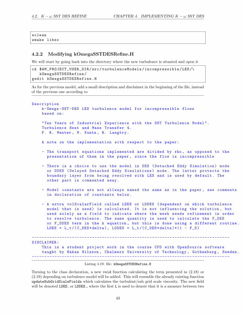
4.2. K − ω SST DES REFINE CHAPTER 4. IMPLEMENTING K − ω SST DES
wclean
wmake libso
4.2.2 Modifying kOmegaSSTDESRefine.H
We will start by going back into the directory where the new turbulence is situated and open it
cd $WM_PROJECT_USER_DIR/src/turbulenceModels/incompressible/LES/\
kOmegaSSTDESRefine/
gedit kOmegaSSTDESRefine.H
As for the previous model, add a small description and disclaimer in the beginning of the file, insteadof the previous one according to
Description
k-Omega -SST -DES LES turbulence model for incompressible flows
based on:
"Ten Years of Industrial Experience with the SST Turbulence Model".
Turbulence Heat and Mass Transfer 4.
F. R. Menter , M. Kuntz , R. Langtry.
A note on the implementation with respect to the paper:
- The transport equations implemented are divided by rho , as opposed to the
presentation of them in the paper , since the flow is incompressible
- There is a choice to use the model in DES (Detached Eddy Simulation) mode
or DDES (Delayed Detached Eddy Simulations) mode. The latter protects the
boundary layer from being resolved with LES and is used by default. The
other part is commented away.
- Model constants are not allways named the same as in the paper , see comments
in declaration of constants below.
- A extra volScalarField called LDES or LDDES (dependent on which turbulence
model that is used) is calculated. It is not influencing the solution , but
used solely as a field to indicate where the mesh needs refinement in order
to resolve turbulence. The same quantity is used to calculate the F_DES
or F_DDES term in the k equation , but this is done using a different routine.
LDES = L_t/( C_DES*delta), LDDES = L_t/( C_DES*delta )*(1 - F_S)
-------------------------------------------------------------------------------
DISCLAIMER:
This is a student project work in the course CFD with OpenSource software
taught by Hakan Nilsson , Chalmers University of Technology , Gothenburg , Sweden.
-------------------------------------------------------------------------------
Listing 4.19: file: kOmegaSSTDESRefine.H
Turning to the class declaration, a new void function calculating the term presented in (2.18) or(2.19) depending on turbulence model will be added. This will resemble the already existing functionupdateSubGridScaleFields which calculates the turbulent/sub grid scale viscosity. The new fieldwill be denoted LDES or LDDES , where the first L is used to denote that it is a measure between two
43
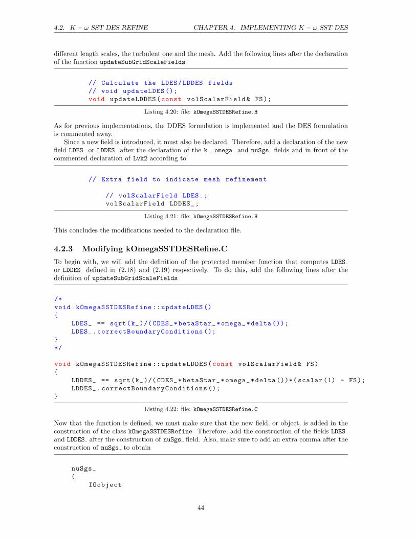
4.2. K − ω SST DES REFINE CHAPTER 4. IMPLEMENTING K − ω SST DES
different length scales, the turbulent one and the mesh. Add the following lines after the declarationof the function updateSubGridScaleFields
// Calculate the LDES/LDDES fields
// void updateLDES ();
void updateLDDES(const volScalarField& FS);
Listing 4.20: file: kOmegaSSTDESRefine.H
As for previous implementations, the DDES formulation is implemented and the DES formulationis commented away.
Since a new field is introduced, it must also be declared. Therefore, add a declaration of the newfield LDES or LDDES after the declaration of the k , omega and nuSgs fields and in front of thecommented declaration of Lvk2 according to
// Extra field to indicate mesh refinement
// volScalarField LDES_;
volScalarField LDDES_;
Listing 4.21: file: kOmegaSSTDESRefine.H
This concludes the modifications needed to the declaration file.
4.2.3 Modifying kOmegaSSTDESRefine.C
To begin with, we will add the definition of the protected member function that computes LDES
or LDDES defined in (2.18) and (2.19) respectively. To do this, add the following lines after thedefinition of updateSubGridScaleFields
/*
void kOmegaSSTDESRefine :: updateLDES ()
LDES_ == sqrt(k_)/( CDES_*betaStar_*omega_*delta ());
LDES_.correctBoundaryConditions ();
*/
void kOmegaSSTDESRefine :: updateLDDES(const volScalarField& FS)
LDDES_ == sqrt(k_)/( CDES_*betaStar_*omega_*delta ())*( scalar (1) - FS);
LDDES_.correctBoundaryConditions ();
Listing 4.22: file: kOmegaSSTDESRefine.C
Now that the function is defined, we must make sure that the new field, or object, is added in theconstruction of the class kOmegaSSTDESRefine. Therefore, add the construction of the fields LDES
and LDDES after the construction of nuSgs field. Also, make sure to add an extra comma after theconstruction of nuSgs to obtain
nuSgs_
(
IOobject
44
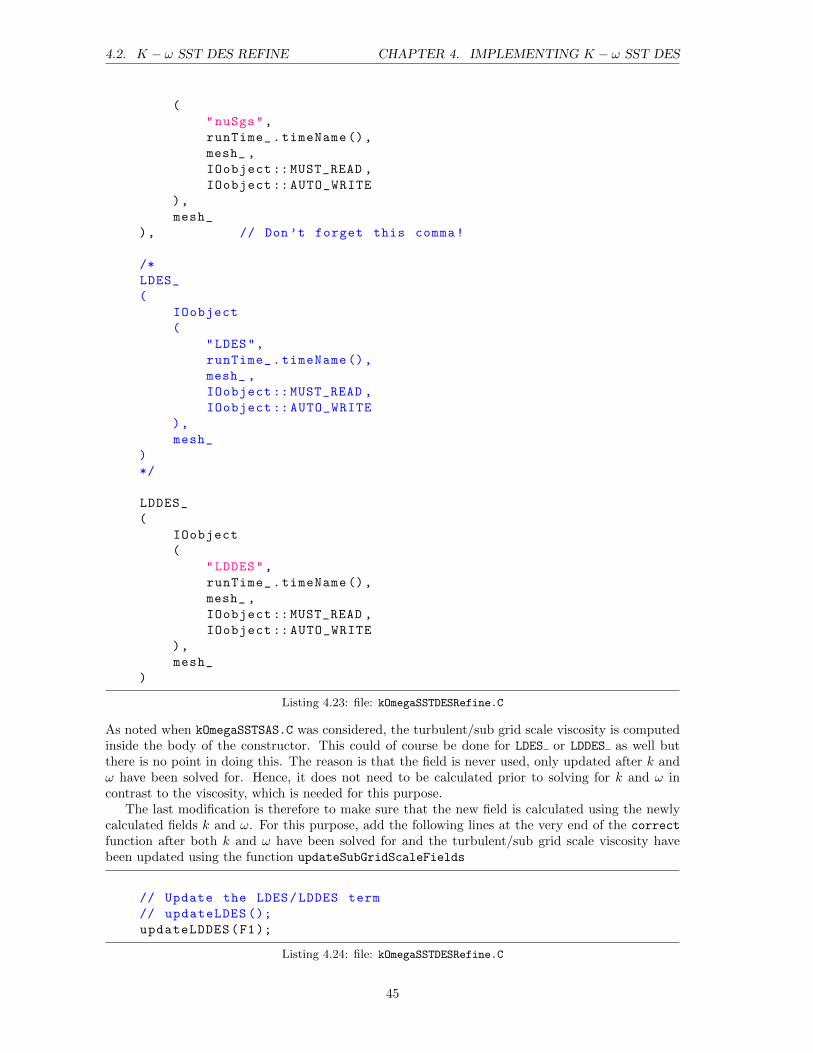
4.2. K − ω SST DES REFINE CHAPTER 4. IMPLEMENTING K − ω SST DES
(
"nuSgs",
runTime_.timeName(),
mesh_ ,
IOobject ::MUST_READ ,
IOobject :: AUTO_WRITE
),
mesh_
), // Don’t forget this comma!
/*
LDES_
(
IOobject
(
"LDES",
runTime_.timeName(),
mesh_ ,
IOobject ::MUST_READ ,
IOobject :: AUTO_WRITE
),
mesh_
)
*/
LDDES_
(
IOobject
(
"LDDES",
runTime_.timeName(),
mesh_ ,
IOobject ::MUST_READ ,
IOobject :: AUTO_WRITE
),
mesh_
)
Listing 4.23: file: kOmegaSSTDESRefine.C
As noted when kOmegaSSTSAS.C was considered, the turbulent/sub grid scale viscosity is computedinside the body of the constructor. This could of course be done for LDES or LDDES as well butthere is no point in doing this. The reason is that the field is never used, only updated after k andω have been solved for. Hence, it does not need to be calculated prior to solving for k and ω incontrast to the viscosity, which is needed for this purpose.
The last modification is therefore to make sure that the new field is calculated using the newlycalculated fields k and ω. For this purpose, add the following lines at the very end of the correct
function after both k and ω have been solved for and the turbulent/sub grid scale viscosity havebeen updated using the function updateSubGridScaleFields
// Update the LDES/LDDES term
// updateLDES ();
updateLDDES(F1);
Listing 4.24: file: kOmegaSSTDESRefine.C
45

4.2. K − ω SST DES REFINE CHAPTER 4. IMPLEMENTING K − ω SST DES
This concludes the creation of the kOmegaSSTDESRefine model. After saving and closing, removethe kOmegaSSTDESRefine.dep file and then go to the directory containing the turbulence modelsand the Make directory and type
wclean
wmake libso
This will rebuild the dynamic library containing the user defined turbulence models to includethe new turbulence model kOmegaSSTDESRefine. Since this model will need a new field in the 0/directory of a case that uses it, please refer to the tutorial section for a guide on how to add this aswell.
46
Chapter 5
Simulation with mesh refinement
This chapter describes how to set up a case to run airfoil simulations with mesh refinement. Itrequires that the reader has implemented the k−ω SST DES turbulence model for mesh refinement(kOmegaSSTDESRefine) according to the previous chapter. The case will be set up so that thesolution can run in either 2 or 3D and with only the pimpleDyMFoam solver. For this purpose, a 2Dmesh of a NACA 4412 airfoil, that is prepared for 3D simulations, have been supplied. At the end,the results of the simulation, both with respect to how the new turbulence model performs and tohow the mesh refinement works, will be presented and briefly discussed.
5.1 Copying files
To begin with, a new OpenFOAM case will be created. Begin by creating a new case by copying anexisting LES tutorial according to
run
cp -r $FOAM_TUTORIALS/incompressible/pisoFoam/les/pitzDaily .
mv pitzDaily Airfoil4412Refine
cd Airfoil4412Refine
Before modifying anything, we will also need a dynamicMeshDict for the pimpleDyMFoam solver.The interDyMFoam solver in OpenFOAM utilizes mesh refinement and hence a dictionary from oneof the interDyMFoam tutorials will be copied into the constant directory.
cp $FOAM_TUTORIALS/multiphase/interDyMFoam/ras/damBreakWithObstacle /\
constant/dynamicMeshDict constant/
Proceed by removing the old blockMeshDict and the boundary file according to
rm constant/polyMesh/blockMeshDict
rm constant/polyMesh/boundary
In the supplied files to this work, a file called blockMeshDict 4412 2D3D has been supplied. Copythis blockMeshDict into the constant/polyMesh/ directory. When this is done, rename it as wellby typing
mv constant/polyMesh/blockMeshDict_4412_2D3D \
constant/polyMesh/blockMeshDict
This blockMeshDict will by default give a 2D mesh (one cell in third direction) when runningblockMesh. However, the front and back patches of the mesh are not of type empty, but instead oftype cyclic. Hence, cyclic boundary conditions will also be prescribed on all flow fields, but if onlyone cell is present in the third direction the simulation will effectively be 2D. The reason for this is
47
5.2. CREATING THE MESH CHAPTER 5. SIMULATION WITH MESH REFINEMENT
to allow the user to choose either to tun the case 2D and save simulation time, or full 3D to allow formore realistic turbulence to be resolved. To obtain a 3D mesh, the 2D mesh needs to be extruded.This can be accomplished with the utility extrudeMesh in OpenFOAM, which needs a dictionary.This dictionary is acquired by typing
cp $FOAM_APP/utilities/mesh/generation/extrude/extrudeMesh /\
extrudeMeshDict system/
This concludes the copying of all necessary files for the case. These will now be modified in theupcoming sections.
5.2 Creating the mesh
In this section, the mesh will be created and if desired, also extruded to 3D. Start by lettingblockMesh creating the 2D mesh by typing
blockMesh
To be able to extrude the mesh to 3D, we will have to modify the extrudeMeshDict according toour mesh. Open the file with a preferred editor and make the following changes.
1. Comment away constructFrom patch and uncomment constructFrom mesh to obtain
constructFrom mesh;
// constructFrom patch;
// constructFrom surface;
2. Change the source case of the mesh that will be extruded to the current case to obtain
sourceCase "../ Airfoil4412Refine";
3. Tell the extrudeMesh utility that it is the front patch that should be extruded. This will effec-tively just add a set of layers in the third direction, giving a 3D mesh. It is the sourcePatchesand exposedPatchName that should be changed to front and back respectively to obtain
sourcePatches (front );
// If construct from patch: patch to use for back (can be same as sourcePatch)
exposedPatchName back;
4. The mesh will be extruded linearly in the third direction, therefore uncomment the linearNormaloption for extrudeModel, and comment the other options (wedge). The changes should looklike
//- Linear extrusion in point -normal direction
extrudeModel linearNormal;
//- Wedge extrusion. If nLayers is 1 assumes symmetry around plane.
// extrudeModel wedge;
5. The amount of layers added on the front is specified by nLayers. The new mesh will thereforecontain nLayers + 1 cells in the third direction after extrusion. Specify this parameter toobtain the desired amount of cells, the author chose 10, according to
nLayers 10;
48
5.3. THE 0/ DIRECTORY CHAPTER 5. SIMULATION WITH MESH REFINEMENT
6. Set the expansion ratio for the new layers added to 1.0 according to
expansionRatio 1.0;
7. There are a lot of different ways extrudeMesh can operate on the mesh, requiring a lot ofdifferent coefficients to be specified for different cases. This extrusion only needs the coefficientspecified within linearNormalCoeffs. Therefore, comment away all other ”...Coeffs” subdictionaries and make sure that linearNormalCoeffs is uncommented according to
linearNormalCoeffs
thickness 0.1;
Here, the thickness of the added layer was changed to 0.1 as well. The thickness refers to thetotal thickness of all the new layers added, and hence the thickness of one new layer is in thecase of no expansion ration thickness/nLayers. The original mesh have a thickness of 0.01,which will hence be obtained for the added cells here as well.
When this is done, a 3D mesh can be obtained by typing
extrudeMesh
5.3 The 0/ directory
After the mesh has been created, it’s time to specify proper boundary and initial conditions forthe velocity, pressure and turbulent quantities. As the mesh is created, the wing is oriented withit’s leading edge in the positive x direction and it’s low pressure side in the positive y direction asshown in Figure 2.1. The boundary conditions in Table 2.1 together with cyclic boundary conditionsconnecting the front and back patch will be implemented. Note that cyclic boundary conditions mustbe specified in the blockMeshDict as well, i.e. it must be specified that these patches are going tobe connected through cyclic boundary conditions.
To begin with we will change the name of some of the patches in the existing files to fit our mesh.Therefore type the following when standing inside the case directory.
sed -i s/lowerWall/bottom/g 0/U
sed -i s/upperWall/top/g 0/U
sed -i s/lowerWall/bottom/g 0/p
sed -i s/upperWall/top/g 0/p
sed -i s/lowerWall/bottom/g 0/k
sed -i s/upperWall/top/g 0/k
sed -i s/lowerWall/bottom/g 0/ nuSgs
sed -i s/upperWall/top/g 0/ nuSgs
sed -i s/lowerWall/bottom/g 0/ nuTilda
sed -i s/upperWall/top/g 0/ nuTilda
5.3.1 Velocity
The velocity is specified in the file 0/U. The velocity will be set to 1 m/s using the freestreamboundary conditions. Begin by changing the initial value of the velocity to the following
internalField uniform (-1 0 0);
The inlet, outlet, top and bottom patch should all have the same boundary conditions, according to
49
5.3. THE 0/ DIRECTORY CHAPTER 5. SIMULATION WITH MESH REFINEMENT
inlet
type freestream;
freestreamValue uniform (-1 0 0);
After this, it is time to add the wing patch, at which a no slip boundary condition will be applied.Therefore, add the following lines after the last of the previous four boundary conditions.
wing
type fixedValue;
value uniform (0 0 0);
Finally, it is time to add the front and back patch, for which cyclic boundary conditions will beapplied. This is done by first removing the patch called frontAndBack and adding the followinglines
front
type cyclic;
back
type cyclic;
Finish by saving and closing the velocity file.
5.3.2 Pressure
The pressure is specified in the file 0/p. The pressure will be initialized to zero everywhere, andno modification is therefore needed to the initial conditions. Continue by changing the boundaryconditions at the inlet, outlet, top and bottom to freestreamPressure, according to
inlet
type freestreamPressure;
The boundary condition for the wing is set to zero gradient by adding this patch
wing
type zeroGradient;
Finally the boundary cyclic boundary conditions needs to be added. Do this by removing thefrontAndBack boundary condition and add the same lines as for the velocity. Finish by saving andclosing the file.
5.3.3 Turbulent kinetic energy
The turbulent kinetic energy conditions are specified in 0/k. Begin by changing the initial conditionto a very small number according to
50
5.3. THE 0/ DIRECTORY CHAPTER 5. SIMULATION WITH MESH REFINEMENT
internalField uniform 1e-06;
Proceed by setting the initial condition at the inlet, top and bottom according to
inlet
type fixedValue;
value uniform 1e-06;
The outlet should be of type zeroGradient, which means that it should be changed to
outlet
type zeroGradient;
At the wing the turbulence is in theory zero, but for numerical stability we will avoid this and justset it to something very small. Therefore add the following lines to specify the wing
wing
type fixedValue;
value uniform 1e-10; // Avoid zero
Proceed by removing the frontAndBack patch boundary conditions and add the same lines as forthe previous quantities to achieve cyclic boundary conditions over the front and back patch. Saveand close the file.
5.3.4 Turbulent frequency
There is no file for the turbulent frequency, instead we will change the name of the file 0/nuTilda.Begin by changing it’s name
mv 0/ nuTilda 0/ omega
The first modification that will be done to the file is to change the name of the object to omega,giving the following
object omega;
Proceed by changing the unit of the field to 1/s and the initial value of the field to 1 according to
dimensions [0 0 -1 0 0 0 0];
internalField uniform 1;
After this the boundary condition at the inlet, top and bottom should be changed to look like
inlet
type fixedValue;
value uniform 1;
The outlet should be zeroGradient. Therefore, change this boundary condition to the same as forthe turbulent kinetic energy. After this, the wing will be treated with a special wall function for theturbulent frequency. To use this add the following lines for the wing patch
51
5.3. THE 0/ DIRECTORY CHAPTER 5. SIMULATION WITH MESH REFINEMENT
wing
type omegaWallFunction;
Cmu 0.09;
kappa 0.41;
E 9.8;
beta1 0.075;
value uniform 1000;
Finally, remove the boundary condition for frontAndBack and add the cyclic boundary conditionsin accordance with before. Save and close the file.
5.3.5 Turbulent/Sub grid scale viscosity
The turbulent/sub grid scale viscosity conditions is specified in the file 0/nuSgs. Begin by settingthe initial value to 1e-6, corresponding to k/ω.
internalField uniform 1e-6;
Continue by changing the boundary conditions at the inlet, outlet, top and bottom to calculatedaccording to
inlet
type calculated;
value uniform 0;
At the wing, no turbulence is present, therefore add the following lines to prescribe the boundarycondition at the wing
wing
type fixedValue;
value uniform 0;
As always, finish by removing the frontAndBack patch boundary conditions and add those to achievecyclic conditions. After this save and close the file.
5.3.6 LDES/LDDES
A field governing mesh refinement is also needed. It is called LDES or LDDES dependent on if theDES or DDES model is used as described earlier. In this case, it is assumed that the DDES modelis used and hence the field LDDES will be added. To achieve this copy the nuSgs file, then changethe name and dimension of the object according to
cp 0/nuSgs 0/ LDDES
sed -i s/nuSgs/LDDES/g 0/ LDDES
sed -i s/"0 2 -1"/"0 0 0"/g 0/ LDDES
After opening the file change the boundary condition at the inlet, outlet, top and bottom tozeroGradient to achieve
52
5.4. THE DICTIONARIES CHAPTER 5. SIMULATION WITH MESH REFINEMENT
inlet
type zeroGradient;
The zeroGradient condition is used because at a patch, there is no definition of the cell size ∆.Hence, it is better to simply assume that it varies little in the normal direction to the patch instead.Also, this field is not used by the turbulence model as discussed earlier, so it’s value at a boundaryis not important in that sense. At the wing, we however know that this field asymptotically must goto zero, due to that the turbulent kinetic energy does. Hence, it is safe to keep the same boundaryconditions as for the turbulent/sub grid scale viscosity.
5.4 The dictionaries
The next step is to set up the necessary dictionaries. The dictionaries that will modified arecontrolDict, fvSolution, fvSchemes, LESProperties and dynamicMeshDict.
5.4.1 controlDict
We start by changing the name of the solver according to
sed -i s/pisoFoam/pimpleDyMFoam/g system/controlDict
The end time must also be modified. Before enabling mesh refinement, the flow must developproperly since we are dealing with a transient simulation. The wing is 1 m long the the flow ispassing it at 1 m/s, so the end time will be chosen to 3 s in order to let the flow pass the wingseveral times. The change is done according to
sed -i s/0.1/3/g system/controlDict
Further, change the ∆t value to 1 · 10−3
sed -i s/1e -05/1e-03/g system/controlDict
The write control should be set to adjustable, since the ∆t value will be governed by the Courantnumber, hence do the following change
sed -i s/timeStep/adjustableRunTime/g system/controlDict
The time intervals for which the solver will write out the results will be set next. The reader can ofcourse choose this as they wish, for now it will be set to 0.2 s according to
sed -i s/100/0.2/g system/controlDict
Let’s also change the purgeWrite option to only keep the latest solutions written and overwriteolder. Here, this number will be changed to 5
sed -i s/" purgeWrite 0"/" purgeWrite 5"/g system/controlDict
To save some space on the disc, especially in case of a 3D simulation in which the amount cellsquickly become very large, write compression will be enabled
sed -i s/off/compressed/g system/controlDict
After this, open the file in an editor and add the following lines before the functions
53

5.4. THE DICTIONARIES CHAPTER 5. SIMULATION WITH MESH REFINEMENT
adjustTimeStep yes;
maxCo 0.4;
libs (" libmyIncompressibleLESModels.so");
This will enable run-time ∆t adjustment based on the Courant number, and also include the k − ωSST DES turbulence model. Furthermore, since the specified functions in the controlDict will notbe used, they can be commented away as well. Finish by saving and closing the file.
5.4.2 fvSolution
Since the copied case uses the pisoFoam solver and solves for other turbulent quantities this dictio-nary needs some changes as well. Start by changing the name of the solver
sed -i s/PISO/PIMPLE/g system/fvSolution
Also change the name of the turbulent quantity used according to
sed -i s/nuTilda/omega/g system/fvSolution
After this, open the file in an editor. To begin with, change the PIMPLE sub dictionary to includethe following
nOuterCorrectors 1;
nCorrectors 2;
nNonOrthogonalCorrectors 2;
pRefCell 0;
pRefValue 0;
correctPhi yes;
These numbers can not completely be justified by the author. However, some general ideas to whythese settings are applied can be given. First, setting the amount of outer correctors to 1 means thatthe solver will effectively operate in PISO mode, since the amount of times the whole PISO loop willbe done are only 1. This seems reasonable considering that the Courant number is chosen small.Most tutorials available on PISO and PIMPLE use two correctors specified on the second line, andhence it was simply kept this way. The third line is included for two reasons. First, since the meshis very skewed, adding non orthogonal correctors will help with the ”non orthogonal” cells present.Without it, continuity will run the risk of not being properly satisfied, which of course affect theentire solution negatively. Also, it will be used to correct for continuity after mesh refinement hasbeen used, as discussed earlier.
After the specification of the solver used for U, add the following
UFinal
solver PBiCG;
preconditioner DILU;
tolerance 1e-05;
relTol 0;
I.e. simply copy the specifications for the U solver and change the keyword to UFinal instead. Dothe same procedure for the quantities k, B and omega as well.
After this, we must define the type of solver that will be used for the pressure corrector equationentered in correctPhi.H in cases the mesh was refined. This is due to that a separate pressurecorrector equation that solves for the quantity pcorr is used. It may be defined by copying thedefinition of the solver for p and renaming it pcorr to achieve
54
5.4. THE DICTIONARIES CHAPTER 5. SIMULATION WITH MESH REFINEMENT
pcorr
solver PCG;
preconditioner DIC;
tolerance 1e-06;
relTol 0.05;
When this has been done, the type of solver used for pressure will also be used since the currentsolver settings will fail to converge. Therefore, change all the pressure solver settings (p, pFinaland pcorr) to the following settings instead
solver PCG;
preconditioner
preconditioner GAMG;
tolerance 1e-5;
relTol 0;
smoother DICGaussSeidel;
nPreeSweeps 0;
nPostSweeps 2;
nFinestSweeps 2;
cacheAgglomeration false;
nCellsInCoarsestLevel 10;
agglomerator faceAreaPair;
mergeLevels 1;
tolerance 1e-05;
relTol 0;
maxIter 100;
The author however chose to keep the relTol to 0.05 for the solution if p, a choice that howevercan not be justified.
5.4.3 fvSchemes
Some small changes to the schemes used, as well as addition of a few more necessary definitions ofschemes that are missing will be done. Begin by simply changing the name of the turbulent quantityused according to
sed -i s/nuTilda/omega/g system/fvSchemes
Furthermore, the Crank Nicholson time integration scheme will be applied, hence perform the fol-lowing change as well
sed -i s/backward /" CrankNicolson 0.5"/g system/fvSchemes
Next, open the file and add the following Laplacian scheme used in the pressure corrector equationthat will be entered when nNonOrthogonalCorrectors is different from zero
laplacian(rAU ,p) Gauss linear corrected;
laplacian(rAU ,pcorr) Gauss linear corrected;
Finally, add the following line in the sub dictionary called fluxRequired
pcorr ;
Save and close the file.
55
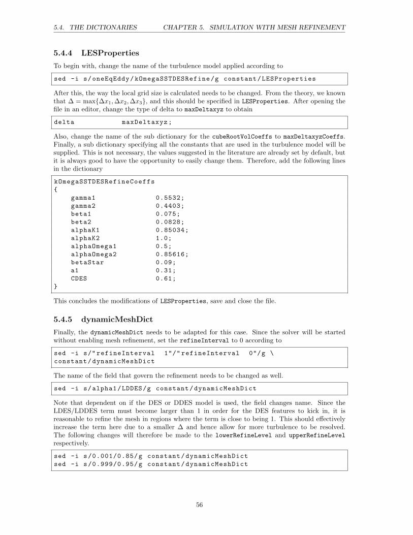
5.4. THE DICTIONARIES CHAPTER 5. SIMULATION WITH MESH REFINEMENT
5.4.4 LESProperties
To begin with, change the name of the turbulence model applied according to
sed -i s/oneEqEddy/kOmegaSSTDESRefine/g constant/LESProperties
After this, the way the local grid size is calculated needs to be changed. From the theory, we knownthat ∆ = max∆x1,∆x2,∆x3, and this should be specified in LESProperties. After opening thefile in an editor, change the type of delta to maxDeltaxyz to obtain
delta maxDeltaxyz;
Also, change the name of the sub dictionary for the cubeRootVolCoeffs to maxDeltaxyzCoeffs.Finally, a sub dictionary specifying all the constants that are used in the turbulence model will besupplied. This is not necessary, the values suggested in the literature are already set by default, butit is always good to have the opportunity to easily change them. Therefore, add the following linesin the dictionary
kOmegaSSTDESRefineCoeffs
gamma1 0.5532;
gamma2 0.4403;
beta1 0.075;
beta2 0.0828;
alphaK1 0.85034;
alphaK2 1.0;
alphaOmega1 0.5;
alphaOmega2 0.85616;
betaStar 0.09;
a1 0.31;
CDES 0.61;
This concludes the modifications of LESProperties, save and close the file.
5.4.5 dynamicMeshDict
Finally, the dynamicMeshDict needs to be adapted for this case. Since the solver will be startedwithout enabling mesh refinement, set the refineInterval to 0 according to
sed -i s/" refineInterval 1"/" refineInterval 0"/g \
constant/dynamicMeshDict
The name of the field that govern the refinement needs to be changed as well.
sed -i s/alpha1/LDDES/g constant/dynamicMeshDict
Note that dependent on if the DES or DDES model is used, the field changes name. Since theLDES/LDDES term must become larger than 1 in order for the DES features to kick in, it isreasonable to refine the mesh in regions where the term is close to being 1. This should effectivelyincrease the term here due to a smaller ∆ and hence allow for more turbulence to be resolved.The following changes will therefore be made to the lowerRefineLevel and upperRefineLevel
respectively.
sed -i s/0.001/0.85/g constant/dynamicMeshDict
sed -i s/0.999/0.95/g constant/dynamicMeshDict
56
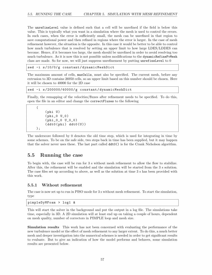
5.5. RUNNING THE CASE CHAPTER 5. SIMULATION WITH MESH REFINEMENT
The unrefineLevel value is defined such that a cell will be unrefined if the field is below thisvalue. This is typically what you want in a simulation where the mesh is used to control the errors.In such cases, when the error is sufficiently small, the mesh can be unrefined in that region tosave computational power and then refined in regions where the error is larger. In the case of meshrefinement however, the situation is the opposite. In this case it would be better to be able to controlhow much turbulence that is resolved by setting an upper limit to how large LDES/LDDES canbecome. Hence, if it becomes too large, the mesh should be unrefined in order to avoid resolving toomuch turbulence. As it is now this is not possible unless modifications to the dynamicRefineFvMeshclass are made. So for now, we will just suppress unrefinement by putting unrefineLevel to 0
sed -i s/10/0/g constant/dynamicMeshDict
The maximum amount of cells, maxCells, must also be specified. The current mesh, before anyextrusion to 3D contains 26950 cells, so an upper limit based on this number should be chosen. Hereit will be chosen to 40000 for the 2D case
sed -i s/200000/40000/g constant/dynamicMeshDict
Finally, the remapping of the velocities/fluxes after refinement needs to be specified. To do this,open the file in an editor and change the correctFluxes to the following
(
(phi U)
(phi_0 U_0)
(phi_0_0 U_0_0)
(ddt0(phi) ddt0(U))
);
The underscore followed by 0 denotes the old time step, which is used for integrating in time bysome schemes. To be on the safe side, two steps back in time has been supplied, but it may happenthat the solver never uses these. The last part called ddt0() is for the Crank Nicholson algorithm.
5.5 Running the case
To begin with, the case will be run for 3 s without mesh refinement to allow the flow to stabilize.After this, the refinement will be enabled and the simulation will be started from the 3 s solution.The case files set up according to above, as well as the solution at time 3 s has been provided withthis work.
5.5.1 Without refinement
The case is now set up to run in PISO mode for 3 s without mesh refinement. To start the simulation,type
pimpleDyMFoam > log1 &
This will start the solver in the background and put the output in a log file. The simulations taketime, especially in 3D. A 2D simulation will at least end up on taking a couple of hours, dependenton mesh quality, number of correctors in PIMPLE loop and mesh size.
Simulation results This work has not been concerned with evaluating the performance of thenew turbulence model or the effect of mesh refinement to any larger extent. To do this, a much bettermesh and deeper investigation into the numerical schemes is needed in order to get significant resultsto evaluate. But to give an indication of how the model performs and behaves, some simulationresults are presented below.
57

5.5. RUNNING THE CASE CHAPTER 5. SIMULATION WITH MESH REFINEMENT
(a) Velocity. (b) Pressure.
Figure 5.1: Velocity and pressure for NACA 4412 Airfoil, ReL = 1 · 105.
(a) Turbulent kinetic energy, k. (b) LDDES .
Figure 5.2: Turbulent kinetic energy and LDDES field for NACA 4412 Airfoil, ReL = 1 · 105.
5.5.2 Enabling refinement
After the flow has stabilized, its time to enable mesh refinement. Do this by changing the parameterrefineInterval from 0 to 10 according to
sed -i s/" refineInterval 0"/" refineInterval 10"/g \
constant/dynamicMeshDict
Also change the start and end time of the simulation according to
sed -i s/" startFrom startTime "/" startFrom latestTime "/g \
system/controlDict
sed -i s/" endTime 3"/" endTime 4"/g \
system/controlDict
After this is done, start the solver again by typing
pimpleDyMFoam > log2 &
Simulation Results The results after mesh refinement are shown below
58
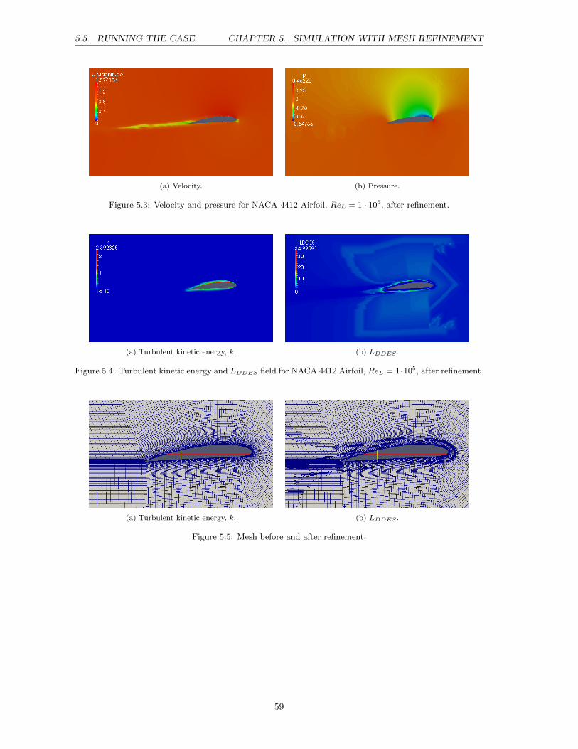
5.5. RUNNING THE CASE CHAPTER 5. SIMULATION WITH MESH REFINEMENT
(a) Velocity. (b) Pressure.
Figure 5.3: Velocity and pressure for NACA 4412 Airfoil, ReL = 1 · 105, after refinement.
(a) Turbulent kinetic energy, k. (b) LDDES .
Figure 5.4: Turbulent kinetic energy and LDDES field for NACA 4412 Airfoil, ReL = 1·105, after refinement.
(a) Turbulent kinetic energy, k. (b) LDDES .
Figure 5.5: Mesh before and after refinement.
59
Chapter 6
Conclusions
This work has involved a variety of topics within the scope of CFD and OpenFOAM, both withrespect to theory, performing simulations and implementation of code.
To begin with the DES formulation of the k − ω SST model was presented with the aim ofdescribing how it works. The conclusion was that the model is designed to resolve turbulence if themesh allows in what is known as the LES mode and otherwise model all the turbulence using theoriginal URANS model. Also from the theory it was noted that OpenFOAM includes the special wallfunctions used for the turbulent frequency which made it possible to easily assign proper boundaryconditions to ω. The simulation was further set to be an airfoil traveling through a still fluid. Thissetting is not realistic in real life applications in which unsteadiness in the air is likely to be present,but allowed for a convenient and fairly easy case to set up. The aim of this project was also not toevaluate the model.
The description of the OpenFOAM implementation regarded a turbulence model, mesh refine-ment and a dynamic mesh solver. The turbulence model implementations in OpenFOAM are alittle bit tricky to understand at first. However, after some training it is fairly easy to understandboth how to modify them as well as to see what equations are actually set up and solved. This is agreat advantage with OpenFOAM, since it allows the user to have full control over the turbulencemodeling in contrast to closed code software. The implementation of the mesh refinement routinein OpenFOAM appears to be very well implemented and works well even though it appears to notbe completely finished. The main drawback that was found was that the cells selected for meshrefinement, in cases where not all candidate cells could be refined, are not selected based on howlarge the governing field is in the cells. I.e., no intelligent selection appears to be performed to refinecells that are ”in greater need” for refinement. As noted for the solver, it is not originally designedfor refining meshes, but rather for moving meshes. It does however work for reining meshes butcould use some modifications to be better suited.
The implementation of the new turbulence model proved to be convenient. Only the DDESmodel was enabled but the change between DES and DDES is easily made. In general, with onlylimited programming knowledge, it is possible to change the way a turbulence model works, whichof course is a great feature.
The simulations proved that the turbulence model performs as intended, but did not try to doany validation work. It was found that the mesh quality is critical when it comes to to obtaininggood results for DES simulations. A fair amount of work had to be put into obtaining meshes thatproduced good results. In particular, three key aspects of the mesh was found critical. First of allthere is the skewness of the mesh. It was found that a very skewed mesh introduced oscillations inthe flow field, which could only partly be avoided with more non-orthogonal correctors in the solver.Second there is the mesh uniformity. Since the mesh size directly control the source term in the kequation, a smoothly changing mesh size is critical. If the mesh changes a lot in size over a smalldistance, so does the source term, and this does not favor a smooth transition between URANS andLES mode. Last there is the resolution near walls. The DDES model includes a limiter to avoidfine near-wall mesh resolution from triggering LES here. However,this protector is not perfect and
60

CHAPTER 6. CONCLUSIONS
it could still happen that the model starts to resolve turbulence here if the mesh is sufficiently fine.In cases with the DES model, this effect is expected to be even more severe. Therefore, near wallmesh resolution is critical in using the DES model properly and as intended. Finally, as noted, theproper choice of solvers for different quantities, in particular pressure, was found important for fastconvergence.
61
Appendix A
MATLAB program to generateairfoil geometry
The Fortran routine that is used to generate the blockMeshDict can take in an arbitrary airfoilgeometry in a file called Airfoil.data. A MATLAB program was therefore written that generatesan Airfoil.data file based on the NACA four digit standard for cambered airfoils. The programwill generate a cross section shape of the airfoil as a set of discrete points constituting the surface.To give better resolution, the points lie closet together towards the leading edge, where the curvaturegenerally is larger.
The program also plots the final airfoil shape together with the NACA number to allow the userto inspect the shape prior to creating the blockMeshDict. There is also an option to plot the airfoilshape at various angles of attack to see how it looks.
The following parameters are possible to adjust in the program
Table A.1: Parameters that can be adjusted when generating airfoil
Parameter Descriptionm Maximum camberp Location of maximum camber as fraction of lengtht Maximum thicknessc Chord length (length of airfoil)
These parameters describe the shape of the airfoil. A description of how this is done is easilyfound on the internet and will not be presented here.
A list of the MATLAB files provided are listed in the next table
Table A.2: MATLAB files necessary to generate airfoil shape.
File DescriptionNACAxxxx.m Main program. Sets parameters and plot resultsy c calc.m Calculate the asymmetric camber line of the airfoil (mean line)y t calc.m Calculate the thickness of the airfoildy c dx calc.m Calculates the gradient, or normal, to the camber lineprofile calc.m Calculates the final profile
62
Appendix B
Extension of blockMeshDict for 3Dsimulation
The blockMeshDict generated by the Fortran routine is for a 2D geometry, i.e. the front andback of the geometry is empty. The author also found that the orientation of the vertices defin-ing the patches of the boundary was done in the counter clockwise, instead of clockwise direction.Therefore, the part of the blockMeshDict defining the boundary was first rewritten to allow for 2Dsimulations with correctly defined boundaries. It was also rewritten further to allow for 2D simula-tions using cyclic boundary conditions to connect the front and back of the domain. The changesto the boundary definition can be found in the files AddToBlockMeshDictClockOrient.data andAddToBlockMeshDictClockOrientCyclic.data respectively. To use these changes, first generate ablockMeshDict using the Fortran routine, and then substitute the part of it named patches(...);
for the content of the file.
63
Bibliography
[1] Menter, F. R. Kuntz, M. Langtry, R. (2003) Ten Years of Industrial Experience with the SSTTurbulence model. Turbulence, Heat and Mass Transfer 4, p. 624 - 632.
[2] Davidsson, L.(2006) Evaluation of the SST-SAS Model: Channel Flow, Asymmetric Diffuserand Axi-Symmetric Hill. In European Conference on Computational Fluid Dynamics ECCOMASCFD 2006 ; September 5-8, 2006, Egmond aan Zee.
[3] Trimarchi, D. https://www.rocq.inria.fr/MACS/spip.php?rubrique69 (2013-10-05)
[4] Menter, F. R. Carregal Ferreira, J. Esch, T. Konno, B. (2003) The SST Turbulence Model withImproved Wall Treatment for Heat Transfer Predictions in Gas Turbines. In Proceedings of theInternational Gas Turbine Congress 2003 Tokyo; November 3-7, 2003, Tokyo.
[5] Versteeg, H. K. Malalasekera, W. (2007) Computational Fluid Dynamics, The Finite VolumeMethod. Second Edition. Harlow: Pearson Education Limited.
[6] Programmers Guide, Version 2.2.2.http://foam.sourceforge.net/docs/Guides-a4/ProgrammersGuide.pdf
64