Processing for the MIPSGAL 24 μm Survey of the Inner...

Processing for the MIPSGAL 24 μm Survey of the Inner Galactic Plane

D. R. MIZUNO,1 S. J. CAREY,2 A. NORIEGA-CRESPO,2 R. PALADINI,2 D. PADGETT,2 S. SHENOY,2

T. A. KUCHAR,1 K. E. KRAEMER,3 AND S. D. PRICE3

Received 2008 February 28; accepted 2008 July 10; published 2008 August 25

ABSTRACT. We describe improvements to the data processing pipeline for the Spitzer MIPSGAL survey of theGalactic plane. These involve both improvements to the processing of the 24 μm data, in particular the handling ofsaturations and near-saturated data, and mitigation of various artifacts not corrected in the basic calibration pipeline.The artifacts addressed postpipeline are typically caused by passage across bright point sources very common in theGalactic plane, and include column-to-column “jailbar” striping, latency effects resulting in both short-durationafterimages and long-duration responsivity depressions, scattered light, and background-level mismatches. Wedescribe the artifacts phenomenologically and present in detail the algorithms developed to correct them.

1. INTRODUCTION

MIPSGAL is a survey of the inner Galactic plane at 24 and70 μm using theMultiband Imaging Photometer System (MIPS)aboard the Spitzer Space Telescope. Rieke et al. (2004) provide adescription of the MIPS instrument, and Werner et al. (2004)describe the Spitzer spacecraft. The scientific objectives, obser-ving strategy, data products, and early results of the MIPSGALproject are described elsewhere (Carey, S. J., et al. 2008, inpreparation).

MIPSGAL comprises two separate observing projects:MIPSGAL I (program ID 20597) covered Galactic longitudesl ¼ 10 to 65°, and l ¼ 295 to 350°, to Galactic latitude jbj ≤ 1°.MIPSGAL II (program ID 30594) extended the survey to higherlatitudes, jbj ≤ 3° in the Galactic center region, l ¼ 350 tol ¼ 10°, excluding a 9° × 2° region aligned on the Galactic cen-ter, which was covered in a different project (program ID 20414,principle investigator F. Yusef-Zadah). For survey complete-ness, however, this latter data set has been processed withthe reduction procedures developed for MIPSGAL and is incor-porated into the MIPSGAL data products.

The image products are a set of 353 1:1° × 1:1° mosaics, witha pixel size of 1.25″ and a resolution of 5.6″. The mosaics arecentered at integral Galactic longitudes and half-integral lati-tudes, and are made in tangent plane projections. In additionto the sky mosaics, corresponding images of coverage, uncer-tainty, and data flags are provided. See Carey, S. J., et al. (2008,in preparation) for a complete description. The mosaics are

available from the Infrared Processing and Analysis Center(IPAC).4

This paper details the steps involved in processing the raw24 μm data into the final mosaics. Section 2 provides a briefoutline. The 70 μm data set requires very different processing,due primarily to the responsivity variations in the Ge:Ga arrays,and is the subject of a separate paper (Paladini R., et al. 2008, inpreparation).

The processing presented here falls into two general cate-gories: calibration and artifact mitigation. A comprehensive dis-cussion of the standard calibration steps is outside the scope ofthis paper (see Gordon et al. 2005), but we have made modifica-tions to the Basic Calibrated Data (BCD) pipeline, in particularimprovements to the linearity correction, droop correction, andhandling of saturated pixels. These are presented in § 3.

The 24 μm data set suffers from a number of residual artifactsthat are not addressed in the basic calibration, among them la-tency effects, in which passage across a bright source causes bothshort-term bright afterimages and a long-term responsivitydepression, column-by-column “jailbar” striping, and scatteredlight on the array due to point sources just out of the field of view.Most of these artifacts are caused bybright sources passing acrossor near the Si:As array, and the high density of bright sources inthe inner Galactic plane makes these artifacts ubiquitous.

The MIPS Data Handbook5 describes mitigation techniquesfor some of these artifacts, but these techniques are either inade-quate for the highly structured backgrounds in the MIPSGALdata or are insufficiently effective, and have not been employedin the current processing.

1Boston College, Institute for Scientific Research, Chestnut Hill, MA, 02467-3800; [email protected]

2 Spitzer Science Center, California Institute of Technology, Pasadena, CA,91125; [email protected], [email protected], [email protected], [email protected]

3 Air Force Research Laboratory, Hanscom AFB, MA, 01731-3010; [email protected]

4 Mosaics are available at http://irsa.ipac.caltech.edu/data/SPITZER/MIPSGAL.

5The MIPS Data Handbook is available at http://ssc.spitzer.caltech.edu/mips/dh/.

1028

PUBLICATIONS OF THE ASTRONOMICAL SOCIETY OF THE PACIFIC, 120:1028–1042, 2008 September© 2008. The Astronomical Society of the Pacific. All rights reserved. Printed in U.S.A.

Instead, we have developed artifact mitigation methods tai-lored for the MIPSGAL data set. The large amount of data in theMIPSGAL survey necessitates that the correction proceduresfor these artifacts be as automated as possible. These proceduresare detailed in § 4.

Section 5 explains a procedure for correcting background-level discrepancies among the approximately half-million dataframes in the survey by minimizing the differences in the frame-to-frame overlaps, so that the resulting mosaics have consistentlevels. Section 6 addresses residual errors in the artifact correc-tions, and § 7 briefly discusses the effectiveness of the correc-tions and provides a summary.

While the artifact corrections have been tailored to the con-ditions in the Galactic plane, the correction procedures, in par-ticular those for the jailbars and latency effects, are very generaland can be applied to other MIPS data sets. The background-level correction mechanism, in addition, can be applied to otherspace-based data; the Spitzer Infrared Array Camera (IRAC),for example, needs a similar correction.

2. OBSERVATION AND PROCESSING OVERVIEW

TheMIPS 24 μm instrument is based on a 128 × 128 array ofSi:As detectors. The field of view of each pixel is 2.55″ on aside, giving a 5.4′ field for the array. For the MIPSGAL project,3 s integrations were used for each frame of data. Transmitted tothe ground for each frame are a slope and first-difference image(explained in § 3.1 below). The Basic Calibrated Data (BCD)pipeline converts these images into a single frame of calibrateddata (hereafter BCD frame or just BCD), along with a corre-sponding uncertainty image, and a BCD mask image that usesbit planes to store per-pixel flags such as saturation, likelylatency effects, and other conditions.

Observations are performed in units called AstronomicalObservation Requests (AORs), which specify integration, point-ing, and scanning parameters for the telescope. For MIPSGAL,the fast scan-mapping mode was used (see the Spitzer Obser-ver’s Manual6 for details), tiling the survey region with scans4 to 6 degrees in length oriented obliquely to the Galactic planeat an angle of ∼66° east of Galactic north-south. Each AOR con-sisted of 3 or 4 scan legs. Each line-of-sight in the survey iscovered at least 5 times in each of 2 scan legs so that eachsky position is imaged in at least 10 BCDs. See Carey, S. J.,et al. (2008, in preparation) for a description of the observingstrategy. MIPSGAL I and II comprise 493 AORs, each with∼1000 BCD frames.

The artifact mitigation is also handled by AORs, in part forconvenience and also for the reason that some artifacts are char-acteristic of the data over complete AORs. The BCDs for eachAOR are passed through a sequence of correction procedures,

each mitigating a particular artifact (§ 4). Following the artifactcorrections, the overall levels of the BCDs are matched in over-lapping regions to ensure background consistency (§ 5). Thecorrected, overlap-matched BCDs are then combined into themosaics using the MOPEX7 software provided by the SpitzerScience Center. The products are the basic sky brightness im-age, coverage and uncertainty images, and a mask image with anaccounting of selected mask flags that affect each mosaic pixel.

The mosaics are inspected visually, with residual artifacts andother problems recorded, and corresponding remedial actions aretaken. The corrections are then reapplied, and the mosaics regen-erated and inspected. The process is repeated as necessary.

3. MIPSGAL BCD PIPELINE

The Spitzer Science Center (SSC) version S14.4 of the BCDpipeline was available at the time the MIPSGAL data were pro-cessed, but the pipeline corrections for linearity and substitutionof the first-difference pixel values (described in § 3.2) were notoptimal, which resulted in the intensities above 300 MJy sr�1 inthat version being unreliable. Instead, in consultation with theMIPS Instrument Support Team at the SSC, we developed anoffline version of the BCD pipeline that provides these correc-tions using the raw data and calibration files available fromLeopard, the standard software tool for retrieving data fromthe Spitzer archive.8

Our modified pipeline starts with the raw data, uses the SSCcalibration files, and performs all the basic calibration steps oftheir pipeline: identification of saturated pixels, “read-2” correc-tion, row-droop and droop correction, dark subtraction, electro-nic linearization, flat-fielding, conversion to physical units, andpixel replacement. Gordon et al. (2005) provide a description ofthese steps. The linearity solution implemented in our pipelineis identical to that in SSC pipeline versions S16.1 and later, andin most other respects, our pipeline is identical to the SSC pipe-line. We have, however, made several modifications appropriateto bright, saturation-filled regions of the sky. We have tailoredthe identification of saturated pixels and the droop correction tobetter account for pixels that are saturated in the first difference.

3.1. Data Collection Overview

In the fast scan-mapping mode used for MIPSGAL, theintegrations are for 2.6 s. The accumulating signal in a pixel(data number or DN) is sampled nondestructively 6 times at Δt ¼ 0:52 s intervals, a mode labeled “sampling up the ramp”(SUR) in MIPS nomenclature. Let DN0 through DN5 representthe six sampled values, or “reads.” To save bandwidth, these rawvalues are not transmitted to the ground but are processed

6 The Spitzer Observer’s Manual is available at http://ssc.spitzer.caltech.edu/documents/som/.

7 The MOPEX software is available for download at http://ssc.spitzer.caltech.edu/postbcd/mopex.html.

8 The Leopard user’s guide is available at http://ssc.spitzer.caltech.edu/documents/leopard/.

PROCESSING FOR MIPSGAL 24 ΜM SURVEY 1029

2008 PASP, 120:1028–1042

onboard the spacecraft into two derived quantities (for this pro-cessing, the initial sample, DN0, is discarded due to electronicartifacts, so the effective integration period is about 2 s). Theslope is calculated by linear regression over the five includedsamples DN1 to DN5, and the first-difference is the differenceof the first two. These values are measures of the signal accu-mulation rate and hence the incident brightness on the pixel.

The onboard slope calculation accounts for differential errorsand correlations between the DN (Gordon et al. 2005), but forillustrative purposes here we show a simplified form. For fittinga linear function to five evenly spaced and equally weighteddata points, we have

slope≃�2 × DN1 � DN2 þ DN4 þ 2 × DN5

10(1)

and, to be explicit,

first-difference ¼ DN2 � DN1: (2)

Note that the (simplified) slope calculation is independent ofDN3. The units of both the first-difference and the slope valuesare DN per sampling interval, or DN per read.

The maximum value of DN is the value at which the signalsaturates the analog-to-digital converter, DNmax ¼ 65; 535. If allsamples for a pixel are below DNmax, then both the slope and thefirst-difference will be accurate measures of the pixel bright-ness, although the first-difference will of course be noisier.At higher signal levels, DN5 first begins to saturate and is thenfollowed in turn by the earlier samples. If any of DN5 down toDN3 are saturated (i.e., values fixed at DNmax), then the slopewill be an underestimate but the first-difference will still be va-lid; this extends the dynamic range. If DN2 is saturated, then thefirst-difference will also be an underestimate; we label this con-dition a soft saturation. If DN1 is saturated, then both the slopeand the first-difference return zero; this is a hard saturation.

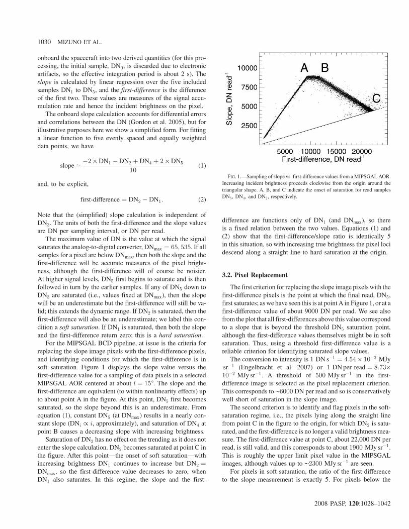
For the MIPSGAL BCD pipeline, at issue is the criteria forreplacing the slope image pixels with the first-difference pixels,and identifying conditions for which the first-difference is insoft saturation. Figure 1 displays the slope value versus thefirst-difference value for a sampling of data pixels in a selectedMIPSGAL AOR centered at about l ¼ 15°. The slope and thefirst-difference are equivalent (to within nonlinearity effects) upto about point A in the figure. At this point, DN5 first becomessaturated, so the slope beyond this is an underestimate. Fromequation (1), constant DN5 (at DNmax) results in a nearly con-stant slope (DNi ∝ i, approximately), and saturation of DN4 atpoint B causes a decreasing slope with increasing brightness.

Saturation of DN3 has no effect on the trending as it does notenter the slope calculation. DN2 becomes saturated at point C inthe figure. After this point—the onset of soft saturation—withincreasing brightness DN1 continues to increase but DN2 ¼DNmax, so the first-difference value decreases to zero, whenDN1 also saturates. In this regime, the slope and the first-

difference are functions only of DN1 (and DNmax), so thereis a fixed relation between the two values. Equations (1) and(2) show that the first-difference/slope ratio is identically 5in this situation, so with increasing true brightness the pixel locidescend along a straight line to hard saturation at the origin.

3.2. Pixel Replacement

The first criterion for replacing the slope image pixelswith thefirst-difference pixels is the point at which the final read, DN5,first saturates; as we have seen this is at point A in Figure 1, or at afirst-difference value of about 9000 DN per read. We see alsofrom the plot that all first-differences above this value correspondto a slope that is beyond the threshold DN5 saturation point,although the first-difference values themselves might be in softsaturation. Thus, using a threshold first-difference value is areliable criterion for identifying saturated slope values.

The conversion to intensity is 1 DN s�1 ¼ 4:54 × 10�2 MJysr�1 (Engelbracht et al. 2007) or 1 DNper read ¼ 8:73×10�2 MJy sr�1. A threshold of 500 MJy sr�1 in the first-difference image is selected as the pixel replacement criterion.This corresponds to ∼6000 DN per read and so is conservativelywell short of saturation in the slope image.

The second criterion is to identify and flag pixels in the soft-saturation regime, i.e., the pixels lying along the straight linefrom point C in the figure to the origin, for which DN2 is satu-rated, and the first-difference is no longer a valid brightness mea-sure. The first-difference value at point C, about 22,000 DN perread, is still valid, and this corresponds to about 1900 MJy sr�1.This is roughly the upper limit pixel value in the MIPSGALimages, although values up to ∼2300 MJy sr�1 are seen.

For pixels in soft-saturation, the ratio of the first-differenceto the slope measurement is exactly 5. For pixels below the

FIG. 1.—Sampling of slope vs. first-difference values from aMIPSGALAOR.Increasing incident brightness proceeds clockwise from the origin around thetriangular shape. A, B, and C indicate the onset of saturation for read samplesDN5, DN4, and DN2, respectively.

1030 MIZUNO ET AL.

2008 PASP, 120:1028–1042

soft-saturation threshold brightness, the ratio is always smallerthan this, monotonically increasing from ∼1 for unsaturateddata up to the soft-saturated value. We use this result to identifysoft-saturated pixels, defining soft saturation as any pixel forwhich the ratio is within 10% of the exact value, i.e., if

first-differenceslope

≥ 4:5; (3)

the pixel is considered soft saturated, and is both flagged in theBCD mask and replaced with the Institute of Electrical andElectronics Engineers (IEEE) Not-a-Number (NaN) value inthe BCD image. Hard-saturated pixels are also flagged andreplaced with the NaN value.

3.3. Droop Correction

The droop is an effect in which the entire array is elevated byan offset, with a magnitude depending on the total signal on thearray. The correction is to total up the pixel values over the array,scale appropriately, and subtract. In the SSC pipeline, the droopoffset is calculated as 0.248 times the mean pixel brightnessover the array (Gordon et al. 2005), and that coefficient is car-ried through in our pipeline.

The presence of saturated pixels, however, lowers the mea-sured total from the true total signal as these pixels always havelower values than the true brightness. With the standard pipe-line, we see the result as elevated background levels in BCDscontaining bright saturated sources.

For soft saturations, the true brightness can be estimated cru-dely with the knowledge of what happens at the onset of satura-tion for DN1 and DN2: When DN2 just saturates, it means thatDNmax is reached after three sample periods (integration starts atabout one sample period prior to DN0). Thus, the true accumu-lation rate is DNmax=3≃ 21; 800 per read, and we see this inFigure 1; point C is at a first-difference value of ∼22; 000DN per read, and is still a valid measure. When DN1 just satu-rates, the true data rate is likewise about DNmax=2 ¼ 32; 768 perread, while the first-difference value drops to zero. The mea-sured values of the first-difference in the soft-saturation regimethus fall in the interval (DNmax=3, 0) and these values map intoan estimated true accumulation rate of (DNmax=3, DNmax=2).Assuming a linear mapping, we have

true-rate≃ DNmax � first-difference2

(4)

in units of DN per read.For the purpose of calculating the total signal in the droop

correction, the soft-saturated pixels are replaced with this esti-mate of the true brightness. Hard-saturated pixels are replacedwith DNmax=2 per read. These substitutions yield a significantimprovement to the correction; a residual droop is typically seenonly in BCDs containing either extremely bright point sources

with large hard-saturated cores, or large regions of hard-saturated extended emission.

4. ARTIFACT MITIGATION

Several significant artifacts remain after the pipeline produc-tion of the basic calibrated data, most of which are inducedby bright sources in or near the BCD frames. The large numberof bright point sources in the MIPSGAL data set precludes asolution such as simply deleting affected frames. The objectiveis to correct the artifacts to whatever extent possible, and thiseffort has been successful in removing the jailbar pattern andbright and dark latency effects from the data. Other artifacts,such as those due to stray light and internal reflections, aretoo irregular to correct, and the solution is to flag the affectedregions of the BCDs in the masks and subsequently omit themfrom the final mosaics.

In this section, we describe each artifact and present themitigation procedure we have developed. A brief discussionof the effectiveness and limitations of the procedures is presentedin § 7.

4.1. Jailbars

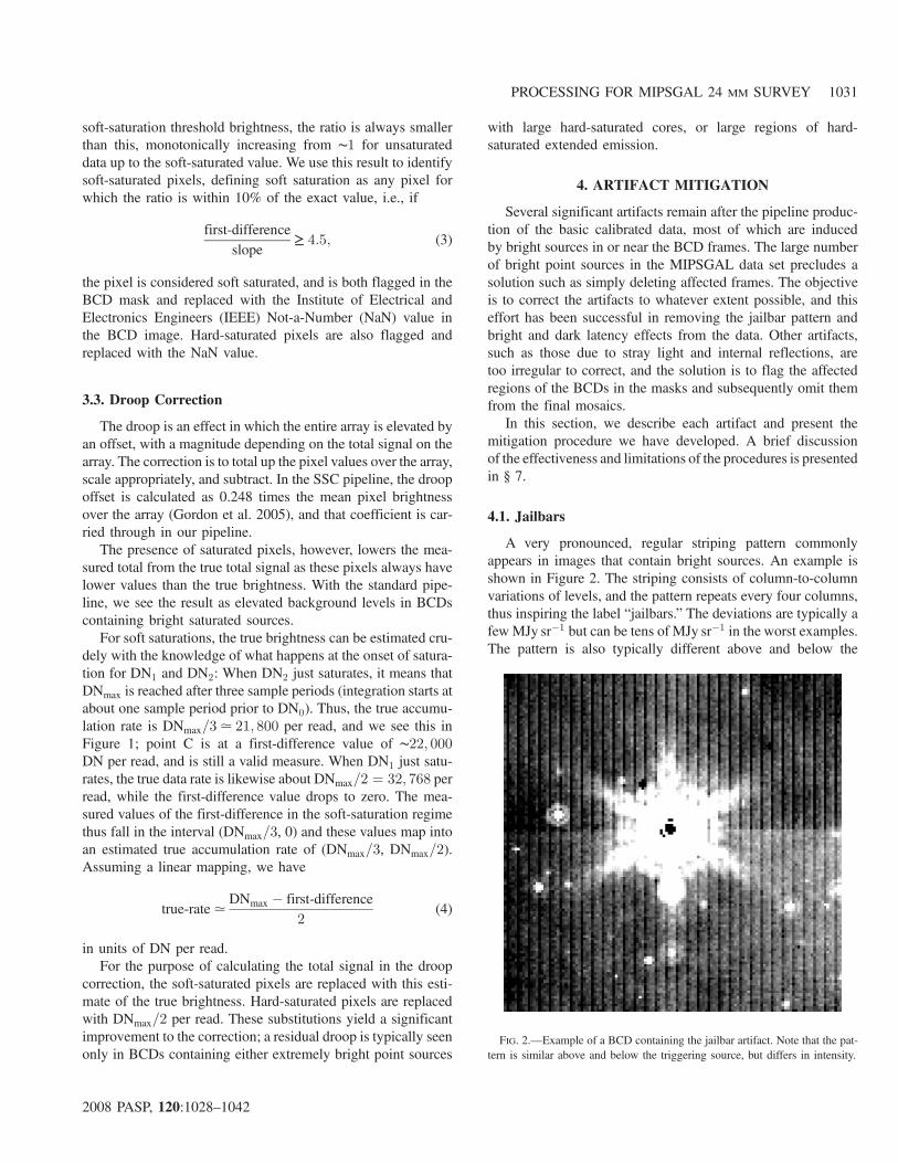
A very pronounced, regular striping pattern commonlyappears in images that contain bright sources. An example isshown in Figure 2. The striping consists of column-to-columnvariations of levels, and the pattern repeats every four columns,thus inspiring the label “jailbars.” The deviations are typically afew MJy sr�1 but can be tens of MJy sr�1 in the worst examples.The pattern is also typically different above and below the

FIG. 2.—Example of a BCD containing the jailbar artifact. Note that the pat-tern is similar above and below the triggering source, but differs in intensity.


2008 PASP, 120:1028–1042

presumed triggering point source, as shown in the figure. Innearly all cases, the jailbar pattern has a single bright-sourcetrigger and consists of differing above-and-below sections,but a few cases have been observed of two triggering sourcesand three distinct jailbar sections. The jailbar effect is always adepression of levels in the columns.

No minimum point source flux for causing this effect hasbeen determined, but it is very seldom seen with sources thatare not saturated at the center (≲4 Jy) and very common withsources >10 Jy. Large regions of saturated extended emissioncan also cause jailbars. There is no direct correlation of thebrightness of a source and the strength of the jailbar pattern;a given source will usually be scanned over several successiveBCDs, and the pattern can be different in all of them. The pat-tern is often worst when the source is near the top or bottom ofthe array, but there is otherwise no general rule.

No cause for this effect has been identified, but the pattern isclearly related to how the pixels in the Si:As array are read out.The pixels are read out in four channels, each readout channelconsisting of 32 columns of the 128 total. The columns are in-terleaved such that each readout samples every fourth column inthe array. When a very bright source falls on the array, we pos-tulate that the pixels in a given readout are depressed by anamount depending in some way on the fluence on the brightestpixel in the readout. As there will generally be differing bright-est pixels in the separate readouts, there will likewise be differ-ing depressions, thus producing a striping pattern in the BCDthat is repeated every four columns.

Engelbracht et al. (2007) suggest that the differing above-and-below pattern is a consequence of two jailbar triggers,one a bright but unsaturated point source, or cosmic ray, whichaffects the whole array, and the other—the obvious saturatedsource in the image—which alters the pattern following the readof the saturated pixels, i.e., above the source in the array. Thiswould imply, however, that uniform jailbar patterns in theabsence of a saturated source should be very common, but infact are comparatively rare in the MIPSGAL data.

Whatever the origin of the jailbar effect, the mitigationmakes use of its phenomenological characteristics. The stripingis due to differential depressions of levels over entire readouts,and so the correction is a global adjustment to each of the read-outs in a section. The interleaving of the readout columns meansthat, in a given BCD, the columns of each readout collectivelyobserve approximately the same region of the sky. Afterremoval of any global gradient, the differences in the readoutmedians are assumed to solely reflect any jailbar errors; residualdifferences due to true sky brightness variations between thereadouts are presumed small enough to ignore.

The steps in the jailbar correction for each BCD are:

1. Remove flat-field correction.The jailbar deviations are uni-form in a readout before the BCD pipeline flat-field correction.

2. Select section boundaries. Array rows containing hard orsoft saturations are considered potential boundaries (i.e., cross a

triggering source). Contiguous rows containing a saturation arecollapsed to a single assumed boundary. The regions betweenboundaries are the jailbar sections. If there are no saturations,the row containing the peak pixel in the array is considered theboundary. Multiple boundaries are allowed, but a minimum of 5rows per jailbar section is imposed.

3. Determine corrections per section. The readout mediansare calculated after removal of any overall gradient in thesection. As the jailbar effect is a depression, the peak readoutmedian is considered closest to truth, and the corrections for theother three readouts are the additive offsets necessary to matchthe peak readout. The depressions are typically up to a fewMJy sr�1 in magnitude.

4. Resolve boundaries. The precise transition point of thejailbar patterns between sections is not known in advance, assaturations usually cover several rows and the transition can oc-cur in any of them. All possible transition points are tested, andthe one yielding the lowest variance in the corrected image overthe potential transition rows is selected.

5. Apply corrections, and reapply flat field.

Note that there is no selection process to distinguish whichBCDs suffer from jailbars. All BCDs are passed through thejailbar correction procedure.

To investigate the effect of the jailbar correction on jailbar-free BCDs, the correction procedure was applied to two AORs,one containing quiescent backgrounds (at l ∼ 55°) and one withbright, structured backgrounds (at l ∼ 8°). The data arrays wererotated by 90° to ensure that no jailbars would be present in theBCDs (the presence of horizontal stripes should have no effecton the jailbar correction). The resulting jailbar “corrections” arethen a measure of the error in the correction mechanism.

The threshold for visual detection of jailbar effects in a givenBCD is a readout-to-readout rms of ∼0:1 MJy sr�1. For thequiescent AOR, the median rms in the resulting readout correc-tions was about 0:02 MJy sr�1, and the worst rms was half thedetection threshold. For the brighter AOR, the median correc-tion rms was the same, but about 1% of the BCDs fell betweenone and 3 times the threshold. In all these cases, however, theBCD contained extremely bright structured emission so that theadded jailbar pattern was not visually detectable.

Also, the jailbar correction added a very small overall bias tothe BCDs, from ∼0:1 MJy sr�1 for the quiescent BCDs to∼0:2 MJy sr�1 for the bright, structured ones. This is perhapsnot surprising as the jailbar correction is always positive. Theabsolute background levels in the BCDs are not known to thisprecision—the uncertainty in the Zodiacal model (Kelsall et al.1998) is ∼10% and so this alone gives an uncertainty ≥1 MJysr�1 for MIPSGAL, and we therefore conclude that the jailbarcorrection is not adding visually detectable artifacts to the data.

For jailbar examples of light to moderate severity, the peakreadout is indeed close to the truth (i.e., in such cases, the peakreadout is unaffected by the jailbar depression), and thecorrection generally results in proper levels in the sections both

1032 MIZUNO ET AL.

2008 PASP, 120:1028–1042

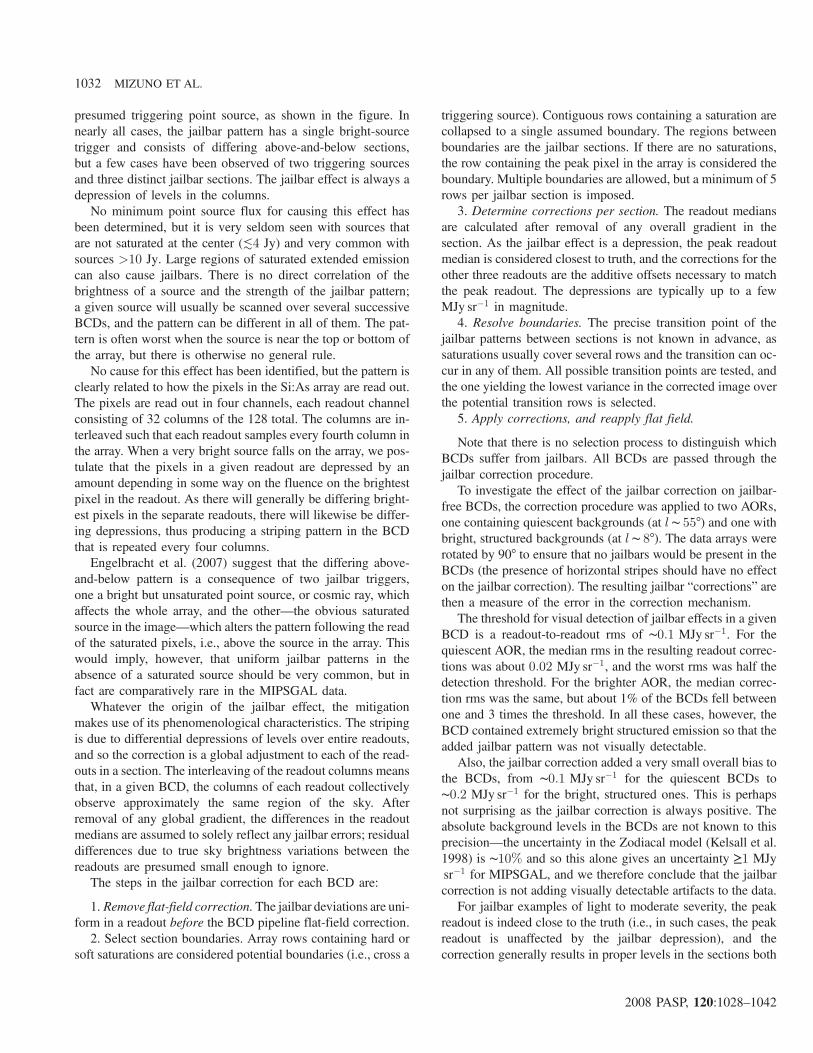
above and below the triggering source. In more severe exam-ples, however, all the readouts suffer from some level depres-sion, and matching to the peak readout still leaves an overalllevel error. Moreover, the effect will generally differ aboveand below the source, and so there will often be a residual dis-continuity of levels across the source after the correction, eventhough the jailbar pattern itself has been removed. Figure 3shows before-and-after examples of both these cases.

The situation of residual level errors following the jailbarcorrection are handled in the overlap correction proceduredescribed in § 5.

4.2. Bright Latents

Bright latents are short-duration afterimages that are ob-served as “ghost” sources following passage of the Si:As arrayacross a bright source. When pixels in the array are exposed tohigh brightness levels in a given BCD, those array pixels arebiased in the immediately subsequent BCD by about 1% ofthe original observed brightness, ∼0:3% in the second BCD thatfollows, and decreasing quasi-exponentially for each BCDthereafter. While the effect is most visible for bright localizedsources, it is assumed that this phenomenon occurs at all inci-dent brightness levels, though smooth extended emission willcause no obvious artifact.

In the MIPSGAL survey, the data were taken in scan legs inwhich the pointing is shifted 54″ or about 1=6 of the array extent

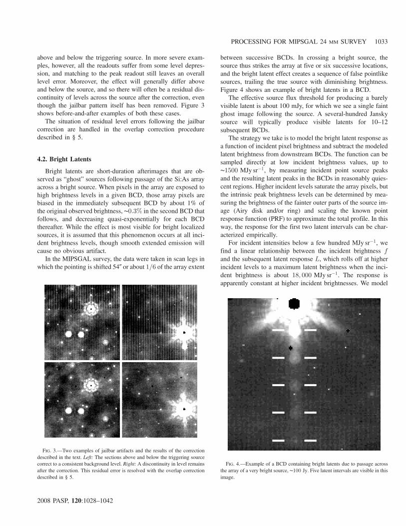
between successive BCDs. In crossing a bright source, thesource thus strikes the array at five or six successive locations,and the bright latent effect creates a sequence of false pointlikesources, trailing the true source with diminishing brightness.Figure 4 shows an example of bright latents in a BCD.

The effective source flux threshold for producing a barelyvisible latent is about 100 mJy, for which we see a single faintghost image following the source. A several-hundred Janskysource will typically produce visible latents for 10–12subsequent BCDs.

The strategy we take is to model the bright latent response asa function of incident pixel brightness and subtract the modeledlatent brightness from downstream BCDs. The function can besampled directly at low incident brightness values, up to∼1500 MJy sr�1, by measuring incident point source peaksand the resulting latent peaks in the BCDs in reasonably quies-cent regions. Higher incident levels saturate the array pixels, butthe intrinsic peak brightness levels can be determined by mea-suring the brightness of the fainter outer parts of the source im-age (Airy disk and/or ring) and scaling the known pointresponse function (PRF) to approximate the total profile. In thisway, the response for the first two latent intervals can be char-acterized empirically.

For incident intensities below a few hundred MJy sr�1, wefind a linear relationship between the incident brightness fand the subsequent latent response L, which rolls off at higherincident levels to a maximum latent brightness when the inci-dent brightness is about 18; 000 MJy sr�1. The response isapparently constant at higher incident brightnesses. We model

FIG. 3.—Two examples of jailbar artifacts and the results of the correctiondescribed in the text. Left: The sections above and below the triggering sourcecorrect to a consistent background level. Right: A discontinuity in level remainsafter the correction. This residual error is resolved with the overlap correctiondescribed in § 5.

FIG. 4.—Example of a BCD containing bright latents due to passage acrossthe array of a very bright source, ∼100 Jy. Five latent intervals are visible in thisimage.


2008 PASP, 120:1028–1042

the trending with an exponential plus a linear term:

L ¼ Að1� e�f0BÞ þ Cf 0; (5)

where

f 0 ¼�f; if f < 18; 00018; 000; if f ≥ 18; 000

; (6)

L and f are in MJy sr�1, and the parametersA,B, andC dependon the specific latent interval. For the first two intervals, L1 andL2, the parameters are determined initially by fitting to theempirical data and are then adjusted manually to give improvedresults in test cases. Table 1 shows the values ofA,B, and C forthe first two latent intervals.

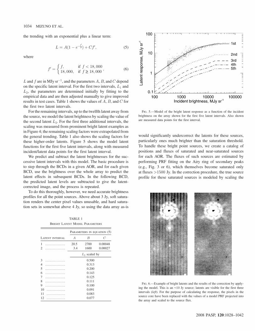
For the remaining intervals, up to the twelfth latent away fromthe source, we model the latent brightness by scaling the value ofthe second latent L2. For the first three additional intervals, thescaling was measured from prominent bright latent examples asin Figure 4; the remaining scaling factors were extrapolated fromthe general trending. Table 1 also shows the scaling factors forthese higher-order latents. Figure 5 shows the model latentfunctions for the first five latent intervals, along with measuredincident/latent data points for the first latent interval.

We predict and subtract the latent brightnesses for the suc-cessive latent intervals with this model. The basic procedure isto step through the BCDs in a given AOR, and for each givenBCD, use the brightness over the whole array to predict thelatent effects in subsequent BCDs. In the following BCD,the predicted latent levels are subtracted to give the latent-corrected image, and the process is repeated.

To do this thoroughly, however, we need accurate brightnessprofiles for all the point sources. Above about 3 Jy, soft satura-tion renders the center pixel values unusable, and hard satura-tion sets in somewhat above 4 Jy, so using the data array as-is

would significantly undercorrect the latents for these sources,particularly ones much brighter than the saturation threshold.To handle these bright point sources, we create a catalog ofpositions and fluxes of saturated and near-saturated sourcesfor each AOR. The fluxes of such sources are estimated byperforming PRF fitting on the Airy ring of secondary peaks(e.g., Fig. 3 or 6), which themselves become saturated onlyat fluxes >1500 Jy. In the correction procedure, the true sourceprofile for these saturated sources is modeled by scaling the

FIG. 6.—Example of bright latents and the results of the correction by apply-ing the model. This is an ∼10 Jy source; latents are visible for the first threeintervals (left). For the purpose of calculating the response, the pixels in thesource core have been replaced with the values of a model PRF projected intothe array and scaled to the source flux.

TABLE 1

BRIGHT LATENT MODEL PARAMETERS

PARAMETERS IN EQUATION (5)

LATENT INTERVAL A B C

1 . . . . . . . . . . . . . . . . 20.5 2700 0.000482 . . . . . . . . . . . . . . . . 3.4 1600 0.00027

L2 scaled by

3 . . . . . . . . . . . . . . . . 0.5004 . . . . . . . . . . . . . . . . 0.3135 . . . . . . . . . . . . . . . . 0.2006 . . . . . . . . . . . . . . . . 0.1437 . . . . . . . . . . . . . . . . 0.1258 . . . . . . . . . . . . . . . . 0.1119 . . . . . . . . . . . . . . . . 0.10010 . . . . . . . . . . . . . . . 0.09111 . . . . . . . . . . . . . . . 0.08312 . . . . . . . . . . . . . . . 0.077

FIG. 5.—Model of the bright latent response as a function of the incidentbrightness on the array shown for the first five latent intervals. Also shownare measured data points for the first interval.

1034 MIZUNO ET AL.

2008 PASP, 120:1028–1042

known PRF to the measured source flux, and projecting the coreinto each BCD array at the appropriate location.

Figure 6 shows an example of the bright latent modelingand subtraction for an ∼10 Jy source, for which the PRF coresubstitution has been applied.

Saturated extended sources remain a problem as we do notknow the profile of a source in the saturated region. In thesecases we replace the saturated array pixels, for the purposeof latent prediction, with a fixed level (4000 MJy sr�1) thatis moderately above the hard-saturation threshold. This providesa partial correction to the bright latents, but leaves residual latenteffects, particularly for very bright compact extended objects.These have not been addressed in the current processing.

4.3. Washboard

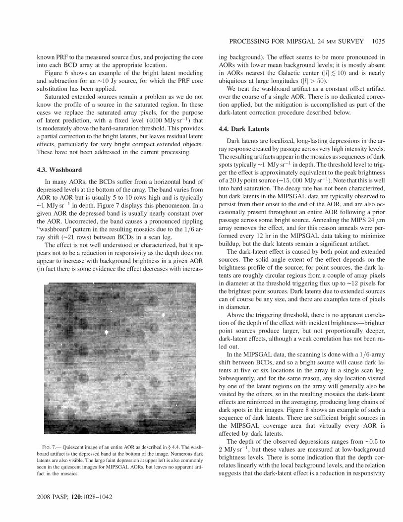
In many AORs, the BCDs suffer from a horizontal band ofdepressed levels at the bottom of the array. The band varies fromAOR to AOR but is usually 5 to 10 rows high and is typically∼1 MJy sr�1 in depth. Figure 7 displays this phenomenon. In agiven AOR the depressed band is usually nearly constant overthe AOR. Uncorrected, the band causes a pronounced rippling“washboard” pattern in the resulting mosaics due to the 1=6 ar-ray shift (∼21 rows) between BCDs in a scan leg.

The effect is not well understood or characterized, but it ap-pears not to be a reduction in responsivity as the depth does notappear to increase with background brightness in a given AOR(in fact there is some evidence the effect decreases with increas-

ing background). The effect seems to be more pronounced inAORs with lower mean background levels; it is mostly absentin AORs nearest the Galactic center (jlj≲ 10) and is nearlyubiquitous at large longitudes (jlj > 50).

We treat the washboard artifact as a constant offset artifactover the course of a single AOR. There is no dedicated correc-tion applied, but the mitigation is accomplished as part of thedark-latent correction procedure described below.

4.4. Dark Latents

Dark latents are localized, long-lasting depressions in the ar-ray response created by passage across very high intensity levels.The resulting artifacts appear in themosaics as sequences of darkspots typically ∼1 MJy sr�1 in depth. The threshold level to trig-ger the effect is approximately equivalent to the peak brightnessof a 20 Jy point source (∼15; 000 MJy sr�1). Note that this is wellinto hard saturation. The decay rate has not been characterized,but dark latents in the MIPSGAL data are typically observed topersist from their onset to the end of the AOR, and are also oc-casionally present throughout an entire AOR following a priorpassage across some bright source. Annealing the MIPS 24 μmarray removes the effect, and for this reason anneals were per-formed every 12 hr in the MIPSGAL data taking to minimizebuildup, but the dark latents remain a significant artifact.

The dark-latent effect is caused by both point and extendedsources. The solid angle extent of the effect depends on thebrightness profile of the source; for point sources, the dark la-tents are roughly circular regions from a couple of array pixelsin diameter at the threshold triggering flux up to ∼12 pixels forthe brightest point sources. Dark latents due to extended sourcescan of course be any size, and there are examples tens of pixelsin diameter.

Above the triggering threshold, there is no apparent correla-tion of the depth of the effect with incident brightness—brighterpoint sources produce larger, but not proportionally deeper,dark-latent effects, although a weak correlation has not been ru-led out.

In the MIPSGAL data, the scanning is done with a 1=6-arrayshift between BCDs, and so a bright source will cause dark la-tents at five or six locations in the array in a single scan leg.Subsequently, and for the same reason, any sky location visitedby one of the latent regions on the array will generally also bevisited by the others, so in the resulting mosaics the dark-latenteffects are reinforced in the averaging, producing long chains ofdark spots in the images. Figure 8 shows an example of such asequence of dark latents. There are sufficient bright sources inthe MIPSGAL coverage area that virtually every AOR isaffected by dark latents.

The depth of the observed depressions ranges from ∼0:5 to2 MJy sr�1, but these values are measured at low-backgroundbrightness levels. There is some indication that the depth cor-relates linearly with the local background levels, and the relationsuggests that the dark-latent effect is a reduction in responsivity

FIG. 7.— Quiescent image of an entire AOR as described in § 4.4. The wash-board artifact is the depressed band at the bottom of the image. Numerous darklatents are also visible. The large faint depression at upper left is also commonlyseen in the quiescent images for MIPSGAL AORs, but leaves no apparent arti-fact in the mosaics.


2008 PASP, 120:1028–1042

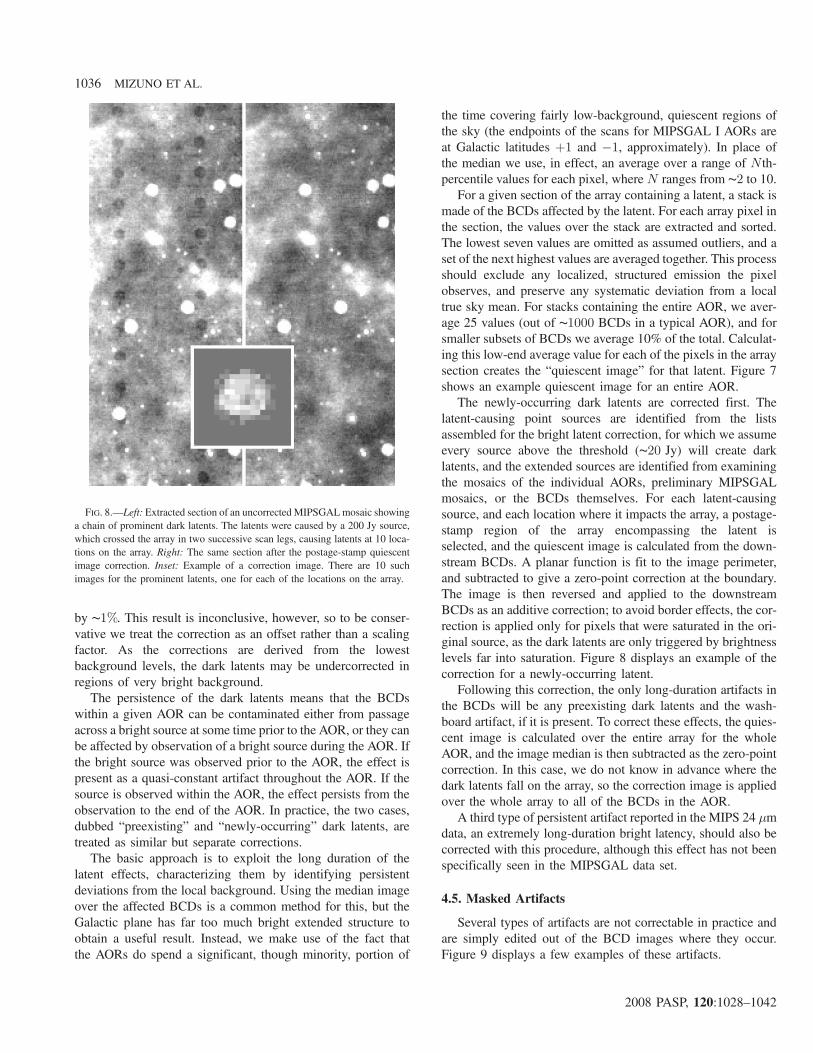
by ∼1%. This result is inconclusive, however, so to be conser-vative we treat the correction as an offset rather than a scalingfactor. As the corrections are derived from the lowestbackground levels, the dark latents may be undercorrected inregions of very bright background.

The persistence of the dark latents means that the BCDswithin a given AOR can be contaminated either from passageacross a bright source at some time prior to the AOR, or they canbe affected by observation of a bright source during the AOR. Ifthe bright source was observed prior to the AOR, the effect ispresent as a quasi-constant artifact throughout the AOR. If thesource is observed within the AOR, the effect persists from theobservation to the end of the AOR. In practice, the two cases,dubbed “preexisting” and “newly-occurring” dark latents, aretreated as similar but separate corrections.

The basic approach is to exploit the long duration of thelatent effects, characterizing them by identifying persistentdeviations from the local background. Using the median imageover the affected BCDs is a common method for this, but theGalactic plane has far too much bright extended structure toobtain a useful result. Instead, we make use of the fact thatthe AORs do spend a significant, though minority, portion of

the time covering fairly low-background, quiescent regions ofthe sky (the endpoints of the scans for MIPSGAL I AORs areat Galactic latitudes þ1 and �1, approximately). In place ofthe median we use, in effect, an average over a range of N th-percentile values for each pixel, where N ranges from ∼2 to 10.

For a given section of the array containing a latent, a stack ismade of the BCDs affected by the latent. For each array pixel inthe section, the values over the stack are extracted and sorted.The lowest seven values are omitted as assumed outliers, and aset of the next highest values are averaged together. This processshould exclude any localized, structured emission the pixelobserves, and preserve any systematic deviation from a localtrue sky mean. For stacks containing the entire AOR, we aver-age 25 values (out of ∼1000 BCDs in a typical AOR), and forsmaller subsets of BCDs we average 10% of the total. Calculat-ing this low-end average value for each of the pixels in the arraysection creates the “quiescent image” for that latent. Figure 7shows an example quiescent image for an entire AOR.

The newly-occurring dark latents are corrected first. Thelatent-causing point sources are identified from the listsassembled for the bright latent correction, for which we assumeevery source above the threshold (∼20 Jy) will create darklatents, and the extended sources are identified from examiningthe mosaics of the individual AORs, preliminary MIPSGALmosaics, or the BCDs themselves. For each latent-causingsource, and each location where it impacts the array, a postage-stamp region of the array encompassing the latent isselected, and the quiescent image is calculated from the down-stream BCDs. A planar function is fit to the image perimeter,and subtracted to give a zero-point correction at the boundary.The image is then reversed and applied to the downstreamBCDs as an additive correction; to avoid border effects, the cor-rection is applied only for pixels that were saturated in the ori-ginal source, as the dark latents are only triggered by brightnesslevels far into saturation. Figure 8 displays an example of thecorrection for a newly-occurring latent.

Following this correction, the only long-duration artifacts inthe BCDs will be any preexisting dark latents and the wash-board artifact, if it is present. To correct these effects, the quies-cent image is calculated over the entire array for the wholeAOR, and the image median is then subtracted as the zero-pointcorrection. In this case, we do not know in advance where thedark latents fall on the array, so the correction image is appliedover the whole array to all of the BCDs in the AOR.

A third type of persistent artifact reported in the MIPS 24 μmdata, an extremely long-duration bright latency, should also becorrected with this procedure, although this effect has not beenspecifically seen in the MIPSGAL data set.

4.5. Masked Artifacts

Several types of artifacts are not correctable in practice andare simply edited out of the BCD images where they occur.Figure 9 displays a few examples of these artifacts.

FIG. 8.—Left: Extracted section of an uncorrected MIPSGALmosaic showinga chain of prominent dark latents. The latents were caused by a 200 Jy source,which crossed the array in two successive scan legs, causing latents at 10 loca-tions on the array. Right: The same section after the postage-stamp quiescentimage correction. Inset: Example of a correction image. There are 10 suchimages for the prominent latents, one for each of the locations on the array.

1036 MIZUNO ET AL.

2008 PASP, 120:1028–1042

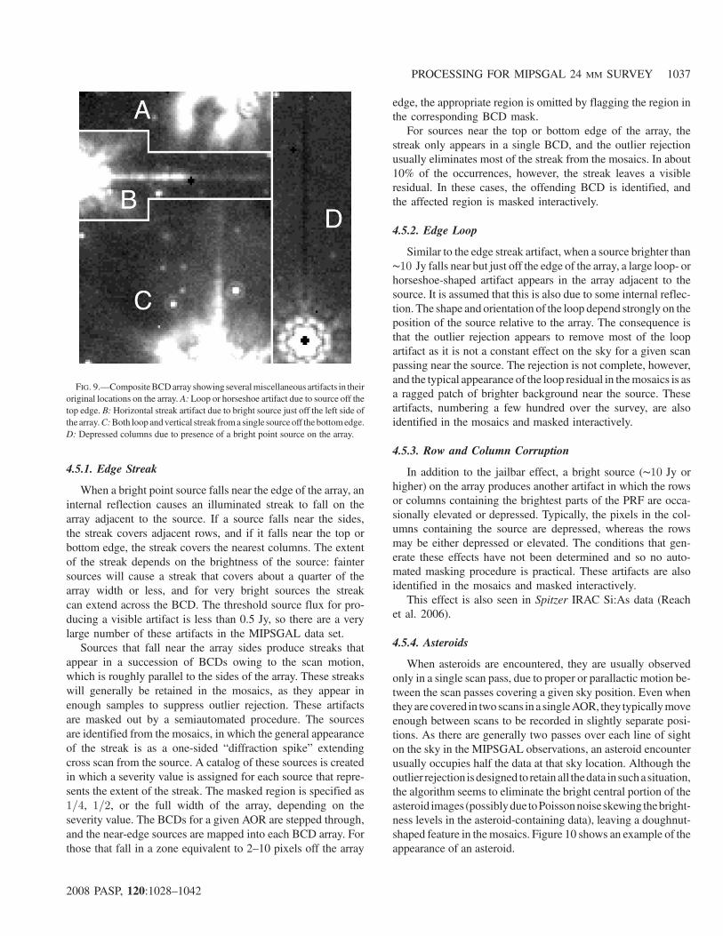
4.5.1. Edge Streak

When a bright point source falls near the edge of the array, aninternal reflection causes an illuminated streak to fall on thearray adjacent to the source. If a source falls near the sides,the streak covers adjacent rows, and if it falls near the top orbottom edge, the streak covers the nearest columns. The extentof the streak depends on the brightness of the source: faintersources will cause a streak that covers about a quarter of thearray width or less, and for very bright sources the streakcan extend across the BCD. The threshold source flux for pro-ducing a visible artifact is less than 0.5 Jy, so there are a verylarge number of these artifacts in the MIPSGAL data set.

Sources that fall near the array sides produce streaks thatappear in a succession of BCDs owing to the scan motion,which is roughly parallel to the sides of the array. These streakswill generally be retained in the mosaics, as they appear inenough samples to suppress outlier rejection. These artifactsare masked out by a semiautomated procedure. The sourcesare identified from the mosaics, in which the general appearanceof the streak is as a one-sided “diffraction spike” extendingcross scan from the source. A catalog of these sources is createdin which a severity value is assigned for each source that repre-sents the extent of the streak. The masked region is specified as1=4, 1=2, or the full width of the array, depending on theseverity value. The BCDs for a given AOR are stepped through,and the near-edge sources are mapped into each BCD array. Forthose that fall in a zone equivalent to 2–10 pixels off the array

edge, the appropriate region is omitted by flagging the region inthe corresponding BCD mask.

For sources near the top or bottom edge of the array, thestreak only appears in a single BCD, and the outlier rejectionusually eliminates most of the streak from the mosaics. In about10% of the occurrences, however, the streak leaves a visibleresidual. In these cases, the offending BCD is identified, andthe affected region is masked interactively.

4.5.2. Edge Loop

Similar to the edge streak artifact, when a source brighter than∼10 Jy falls near but just off the edge of the array, a large loop- orhorseshoe-shaped artifact appears in the array adjacent to thesource. It is assumed that this is also due to some internal reflec-tion. The shape and orientation of the loop depend strongly on theposition of the source relative to the array. The consequence isthat the outlier rejection appears to remove most of the loopartifact as it is not a constant effect on the sky for a given scanpassing near the source. The rejection is not complete, however,and the typical appearance of the loop residual in themosaics is asa ragged patch of brighter background near the source. Theseartifacts, numbering a few hundred over the survey, are alsoidentified in the mosaics and masked interactively.

4.5.3. Row and Column Corruption

In addition to the jailbar effect, a bright source (∼10 Jy orhigher) on the array produces another artifact in which the rowsor columns containing the brightest parts of the PRF are occa-sionally elevated or depressed. Typically, the pixels in the col-umns containing the source are depressed, whereas the rowsmay be either depressed or elevated. The conditions that gen-erate these effects have not been determined and so no auto-mated masking procedure is practical. These artifacts are alsoidentified in the mosaics and masked interactively.

This effect is also seen in Spitzer IRAC Si:As data (Reachet al. 2006).

4.5.4. Asteroids

When asteroids are encountered, they are usually observedonly in a single scan pass, due to proper or parallactic motion be-tween the scan passes covering a given sky position. Even whentheyare covered in twoscans in a singleAOR, they typicallymoveenough between scans to be recorded in slightly separate posi-tions. As there are generally two passes over each line of sighton the sky in the MIPSGAL observations, an asteroid encounterusually occupies half the data at that sky location. Although theoutlier rejection isdesigned to retain all thedata insuchasituation,the algorithm seems to eliminate the bright central portion of theasteroid images (possiblydue toPoissonnoiseskewing thebright-ness levels in the asteroid-containing data), leaving a doughnut-shaped feature in themosaics. Figure 10 shows an example of theappearance of an asteroid.

FIG. 9.—CompositeBCDarray showing severalmiscellaneous artifacts in theiroriginal locations on the array. A: Loop or horseshoe artifact due to source off thetop edge. B:Horizontal streak artifact due to bright source just off the left side ofthe array.C:Both loop andvertical streak froma single source off the bottomedge.D: Depressed columns due to presence of a bright point source on the array.


2008 PASP, 120:1028–1042

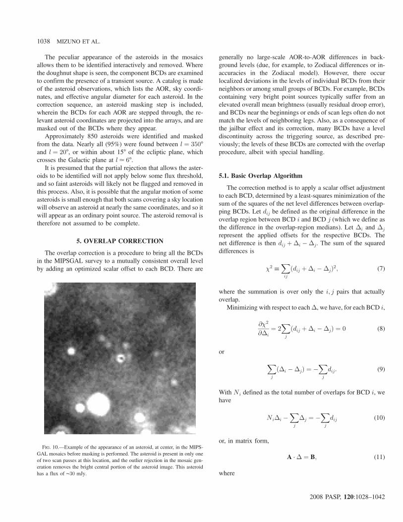
The peculiar appearance of the asteroids in the mosaicsallows them to be identified interactively and removed. Wherethe doughnut shape is seen, the component BCDs are examinedto confirm the presence of a transient source. A catalog is madeof the asteroid observations, which lists the AOR, sky coordi-nates, and effective angular diameter for each asteroid. In thecorrection sequence, an asteroid masking step is included,wherein the BCDs for each AOR are stepped through, the re-levant asteroid coordinates are projected into the arrays, and aremasked out of the BCDs where they appear.

Approximately 850 asteroids were identified and maskedfrom the data. Nearly all (95%) were found between l ¼ 350°and l ¼ 20°, or within about 15° of the ecliptic plane, whichcrosses the Galactic plane at l≃ 6°.

It is presumed that the partial rejection that allows the aster-oids to be identified will not apply below some flux threshold,and so faint asteroids will likely not be flagged and removed inthis process. Also, it is possible that the angular motion of someasteroids is small enough that both scans covering a sky locationwill observe an asteroid at nearly the same coordinates, and so itwill appear as an ordinary point source. The asteroid removal istherefore not assumed to be complete.

5. OVERLAP CORRECTION

The overlap correction is a procedure to bring all the BCDsin the MIPSGAL survey to a mutually consistent overall levelby adding an optimized scalar offset to each BCD. There are

generally no large-scale AOR-to-AOR differences in back-ground levels (due, for example, to Zodiacal differences or in-accuracies in the Zodiacal model). However, there occurlocalized deviations in the levels of individual BCDs from theirneighbors or among small groups of BCDs. For example, BCDscontaining very bright point sources typically suffer from anelevated overall mean brightness (usually residual droop error),and BCDs near the beginnings or ends of scan legs often do notmatch the levels of neighboring legs. Also, as a consequence ofthe jailbar effect and its correction, many BCDs have a leveldiscontinuity across the triggering source, as described pre-viously; the levels of these BCDs are corrected with the overlapprocedure, albeit with special handling.

5.1. Basic Overlap Algorithm

The correction method is to apply a scalar offset adjustmentto each BCD, determined by a least-squares minimization of thesum of the squares of the net level differences between overlap-ping BCDs. Let dij be defined as the original difference in theoverlap region between BCD i and BCD j (which we define asthe difference in the overlap-region medians). Let Δi and Δj

represent the applied offsets for the respective BCDs. Thenet difference is then dij þΔi �Δj. The sum of the squareddifferences is

χ2 ≡Xij

ðdij þΔi �ΔjÞ2; (7)

where the summation is over only the i; j pairs that actuallyoverlap.

Minimizing with respect to eachΔ, we have, for each BCD i,

∂χ2

∂Δi

¼ 2Xj

ðdij þΔi �ΔjÞ ¼ 0 (8)

or

Xj

ðΔi �ΔjÞ ¼ �Xj

dij: (9)

With Ni defined as the total number of overlaps for BCD i, wehave

NiΔi �Xj

Δj ¼ �Xj

dij (10)

or, in matrix form,

A ·Δ ¼ B; (11)

where

FIG. 10.—Example of the appearance of an asteroid, at center, in the MIPS-GAL mosaics before masking is performed. The asteroid is present in only oneof two scan passes at this location, and the outlier rejection in the mosaic gen-eration removes the bright central portion of the asteroid image. This asteroidhas a flux of ∼30 mJy.

1038 MIZUNO ET AL.

2008 PASP, 120:1028–1042

Aij ≡�Ni; if i ¼ j�δij; if i ≠ j

; (12)

δij ≡ 1 if BCDs i and j overlap, zero otherwise, and

Bi ≡�Xj

dij: (13)

This simple system of equations is ill conditioned as the solutionis not unique: any global offset to the set of corrections Δ willalso satisfy equation (9) for all BCDs i. This is not a conceptualdifficulty as we can apply some reasonable condition on Δ as aconstraint (perhaps minimizing the sum of the squares of theΔs), although solving this set of equations for a very large num-ber of BCDs may be computationally problematic. A more ser-ious problem is that the least-squares condition for a single BCD(eq. [9] or [10]) is also individually satisfied with any arbitraryoffset added to the local corrections. This results in the overallsolution being very poorly constrained against large, spuriousgradients in the resulting background levels: if the solutionto the equations requires extreme global variations in the Δs,then that is what we get, although it is unlikely to be physicalin any ordinary circumstances. We typically see this exagger-ated “ramping” result when the BCDs suffer from some sys-tematic inhomogeneity, such as the washboard effect.

5.2. Damped Overlap

The MIPS 24 μm pipeline processing removes instrumentalbias, and so the background levels of the MIPSGAL pipeline-produced BCDs are, collectively, a measure of the absolutebackground. For the overlap correction, therefore, we want topreserve as much as possible the global background as-is, whileremoving BCD-to-BCD differences. To mitigate the potentialramping problem, the approach we take is to include the offsetsthemselves in the minimized function, along with the overlapdifferences, with the intent of suppressing large magnitudesof Δ. We redefine χ2 as

χ2 ≡Xij

ðdij þΔi �ΔjÞ2 þXk

βkðΔkÞ2; (14)

where k is summed over all BCDs, and the βk are selected tocontrol the strength of the damping effect.

The least-squares minimization gives, for each BCD i,

Xj

ðdij þΔi �ΔjÞ þ βiΔi ¼ 0: (15)

If a set of Δs local to BCD i satisfies the original overlapcondition given by equation (8), then this equation is nearlysatisfied also, provided βi is sufficiently small and the net localΔ offset is also small (i.e., no ramping in the solution). Con-versely, a set ofΔs that satisfies this relation also nearly satisfiesequation (8). That is, a solution to this damped set of equations

is also very nearly a solution to the basic overlap correction con-ditions, provided the βs are small enough. The asymmetry ofΔi

in equation (15) assures that the overall level of the local Δcannot be set arbitrarily as part of a global solution becausea uniform offset to theΔ on the left hand side no longer cancels.Also, note that if the BCDs satisfy the minimization condition(eq. [9]) without correction, i.e.,

Pjdij ¼ 0, then equation (15)

is also satisfied with zero correction, and so this procedure willnot add deviations to already-matching data.

In essence, this is an overlap solution that allows smallresidual level differences while largely preserving the globalbackground levels. The fractional deviation of any Δi fromthe “true” value is approximately the fractional change in thecoefficient of Δi on the left hand side of equation (15) fromthat of equation (8), or βi=Ni (provided βi ≪ Ni). In otherwords, the residual overlap difference for BCD i and overlap-ping BCD j after the correction will typically be on the orderof ðβi=NiÞdij.

In practice, βi is set such that the damping effect is indepen-dent of the mean number of overlaps. We set βi ¼ αNi, whereα is a single free parameter specifying the strength of the damp-ing. The damped solution is thus simply a change to the diag-onal elements of the overlap correction matrix, from Aii ¼ Ni

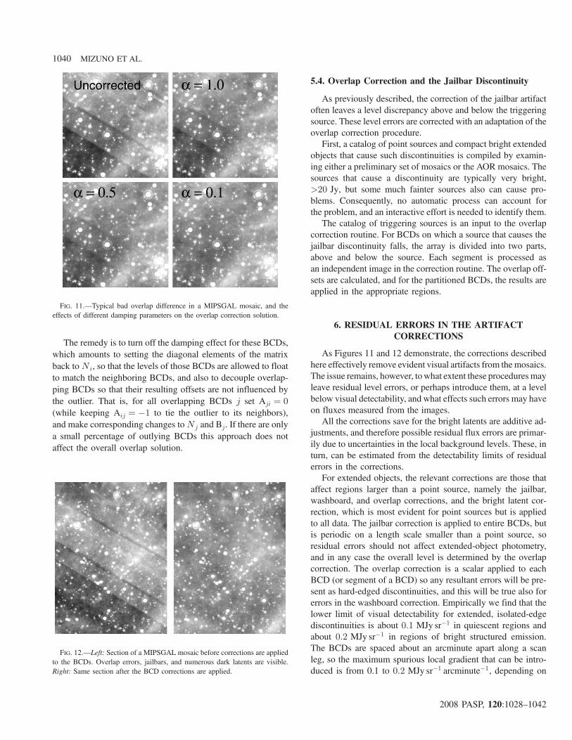
to Aii ¼ Nið1þ αÞ. The optimal value of α depends on the ac-ceptable fractional residual overlap difference. For MIPSGAL,typical uncorrected overlap differences are, at most, on the orderof 2 MJy sr�1, whereas the smallest difference visually detect-able is about 0:1 MJy sr�1, so α for MIPSGAL should be nomore than about 0.05. Figure 11 shows a section of a MIPSGALmosaic containing a “bad” overlap difference, and the overlapcorrection results for several values of α. For α ¼ 1:0, we seevery little correction, as expected; for α ¼ 0:1, the overlapdifferences have been largely eliminated.

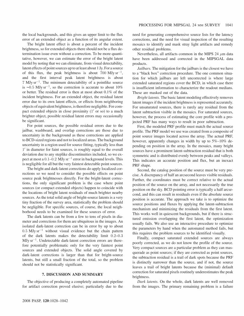
For MIPSGAL, we used α ¼ 0:04. Figure 12 shows abefore-and-after example of the damped overlap correctionfor the same mosaic as Figure 11 but over a larger region.

One benefit of the damping procedure is that the resultingmatrix is well conditioned, and for the MIPSGAL data, it is verysparse, so computationally it is a straightforward solution evenfor very large numbers of BCDs. In the current release, the firstquadrant, fourth quadrant, and Galactic center regions wereprocessed separately; each contained from 150,000 to 190,000BCDs.

5.3. Outliers

Typical overlap differences are 1–2 MJy sr�1, but numerousfairly isolated BCDs deviate from their neighbors by up to tensof MJy sr�1, usually from a residual droop when crossing verybright point sources, or residual jailbar level errors. The dampedoverlap correction itself cannot correct these cases effectively, asthe residual overlap difference would typically remain a visibleartifact; worse, the solution would tend to drag neighboringBCDs up or down to match the deviant BCD.


2008 PASP, 120:1028–1042

The remedy is to turn off the damping effect for these BCDs,which amounts to setting the diagonal elements of the matrixback toNi, so that the levels of those BCDs are allowed to floatto match the neighboring BCDs, and also to decouple overlap-ping BCDs so that their resulting offsets are not influenced bythe outlier. That is, for all overlapping BCDs j set Aji ¼ 0

(while keeping Aij ¼ �1 to tie the outlier to its neighbors),and make corresponding changes toNj and Bj. If there are onlya small percentage of outlying BCDs this approach does notaffect the overall overlap solution.

5.4. Overlap Correction and the Jailbar Discontinuity

As previously described, the correction of the jailbar artifactoften leaves a level discrepancy above and below the triggeringsource. These level errors are corrected with an adaptation of theoverlap correction procedure.

First, a catalog of point sources and compact bright extendedobjects that cause such discontinuities is compiled by examin-ing either a preliminary set of mosaics or the AOR mosaics. Thesources that cause a discontinuity are typically very bright,>20 Jy, but some much fainter sources also can cause pro-blems. Consequently, no automatic process can account forthe problem, and an interactive effort is needed to identify them.

The catalog of triggering sources is an input to the overlapcorrection routine. For BCDs on which a source that causes thejailbar discontinuity falls, the array is divided into two parts,above and below the source. Each segment is processed asan independent image in the correction routine. The overlap off-sets are calculated, and for the partitioned BCDs, the results areapplied in the appropriate regions.

6. RESIDUAL ERRORS IN THE ARTIFACTCORRECTIONS

As Figures 11 and 12 demonstrate, the corrections describedhere effectively remove evident visual artifacts from themosaics.The issue remains, however, towhat extent these proceduresmayleave residual level errors, or perhaps introduce them, at a levelbelow visual detectability, and what effects such errors may haveon fluxes measured from the images.

All the corrections save for the bright latents are additive ad-justments, and therefore possible residual flux errors are primar-ily due to uncertainties in the local background levels. These, inturn, can be estimated from the detectability limits of residualerrors in the corrections.

For extended objects, the relevant corrections are those thataffect regions larger than a point source, namely the jailbar,washboard, and overlap corrections, and the bright latent cor-rection, which is most evident for point sources but is appliedto all data. The jailbar correction is applied to entire BCDs, butis periodic on a length scale smaller than a point source, soresidual errors should not affect extended-object photometry,and in any case the overall level is determined by the overlapcorrection. The overlap correction is a scalar applied to eachBCD (or segment of a BCD) so any resultant errors will be pre-sent as hard-edged discontinuities, and this will be true also forerrors in the washboard correction. Empirically we find that thelower limit of visual detectability for extended, isolated-edgediscontinuities is about 0:1 MJy sr�1 in quiescent regions andabout 0:2 MJy sr�1 in regions of bright structured emission.The BCDs are spaced about an arcminute apart along a scanleg, so the maximum spurious local gradient that can be intro-duced is from 0.1 to 0:2 MJy sr�1 arcminute�1, depending on

FIG. 11.—Typical bad overlap difference in a MIPSGAL mosaic, and theeffects of different damping parameters on the overlap correction solution.

FIG. 12.—Left: Section of a MIPSGAL mosaic before corrections are appliedto the BCDs. Overlap errors, jailbars, and numerous dark latents are visible.Right: Same section after the BCD corrections are applied.

1040 MIZUNO ET AL.

2008 PASP, 120:1028–1042

the local backgrounds, and this gives an upper limit to the fluxerror of an extended object as a function of its angular extent.

The bright latent effect is about a percent of the incidentbrightness, so for extended objects there should not be a flux de-termination issue even without a correction. To be more quanti-tative, however, we can estimate the error of the bright latentmodel by noting that we can eliminate, from visual detectability,latent effects of point sources up to at least about 1 Jy. For a sourceof this flux, the peak brightness is about 700 MJy sr�1,and the first interval peak latent brightness is about7 MJy sr�1. The minimum detectability of a pointlike sourceis ∼0:5 MJy sr�1, so the correction is accurate to about 10%or better. The residual error is then at most about 0.1% of theincident brightness. For an extended object, the residual latenterror due to its own latent effects, or effects from neighboringobjects of equivalent brightness, is therefore negligible. For com-pact extended objects in close proximity (10 or so) to a muchbrighter object, possible residual latent errors may occasionallybe significant.

For point sources, the possible residual errors due to thejailbar, washboard, and overlap corrections are those due touncertainty in the background as these corrections are appliedto BCD-sized regions and not to localized areas. The backgrounduncertainty in a region used for source fitting, typically less than10 in diameter for faint sources, is roughly equal to the overalldeviation due to any steplike discontinuities included, so we ex-pect at most a 0:1–0:2 MJy sr�1 error in background levels. Thisis negligible for all but the very faintest detectable point sources.

The bright and dark-latent corrections do apply localized cor-rections so we need to consider the possible effects on pointsource peak brightnesses directly. For the bright-latent correc-tions, the only significant problem is the case where pointsources (or compact extended objects) happen to coincide withthe locations of bright latent residuals of much brighter nearbysources. As the total solid angle of bright-source latents is a verytiny fraction of the survey area, statistically the problem shouldbe negligible. For specific sources, of course, the local neigh-borhood needs to be examined for these sources of error.

The dark latents can be from a few to tens of pixels in dia-meter and corrections for them are ubiquitous in the images. Anisolated dark-latent correction can be in error by up to about0:5 MJy sr�1 without visual evidence but the chain patternof the dark latents makes the detectability limit 0:2–0:3MJy sr�1. Undetectable dark-latent correction errors are there-fore potentially problematic only for the very faintest pointsources and extended objects. The solid angle covered bydark-latent corrections is larger than that for bright-sourcelatents, but still a small fraction of the total, so the problemshould not be statistically significant.

7. DISCUSSION AND SUMMARY

The objective of producing a completely automated pipelinefor artifact correction proved elusive; particularly due to the

need for generating comprehensive source lists for the latencycorrections, and the need for visual inspection of the resultingmosaics to identify and mask stray light artifacts and remedyother residual problems.

Nevertheless, all artifacts common in the MIPS 24 μm datahave been addressed and corrected in the MIPSGAL dataproducts.

Jailbars. The mitigation for the jailbars is the closest we haveto a “black box” correction procedure. The one common situa-tion for which jailbars are left uncorrected is where largeextended saturated regions cover the BCD, in which case thereis insufficient information to characterize the readout medians.These are masked out of the data.

Bright latents. The basic latent modeling effectively removeslatent images if the incident brightness is represented accurately.For unsaturated sources, there is rarely any residual from thelatent subtraction visible in the mosaics. For saturated sources,however, the process of estimating the core profile with a pro-jected PRF has many ways to result in poor subtraction.

First, the modeled PRF profile must match the actual sourceprofile. The PRF model we use was created from a composite ofpoint source images located across the array. The actual PRF,however, apparently changes in width by up to 5%–10% de-pending on position in the array. In the mosaics, many brightsources have a prominent latent-subtraction residual that is bothsymmetric and is distributed evenly between peaks and valleys.This indicates an accurate position and flux, but an inexactPRF shape.

Second, the catalog position of the source must be very pre-cise. A discrepancy of half an arcsecond leaves visible residuals.Further, the coordinates must be correct relative to the actualposition of the source on the array, and not necessarily the trueposition on the sky. BCD pointing error is typically a half arcse-cond, and this can result in residuals even if the absolute sourceposition is accurate. The approach we take is to optimize thesource positions and fluxes by applying the latent-subtractionmechanism and minimizing the residuals from the first latent.This works well in quiescent backgrounds, but if there is struc-tured emission overlapping the first latent, the optimizationusually fails. We also use an interactive procedure to optimizethe parameters by hand when the automated method fails, butthis requires the problem sources to be identified visually.

Finally, compact saturated extended sources are alwayspoorly corrected, as we do not know the profile of the source.Very compact sources are a particular problem as they can mas-querade as point sources; if they are corrected as point sources,the subtraction residual is a trail of dark spots because the PRFis distinctly narrower than the source, and if not, the sourceleaves a trail of bright latents because the (minimal) defaultcorrection for saturated pixels routinely underestimates the peakbrightness.

Dark latents. On the whole, dark latents are well removedfrom the images. The primary remaining problem is a failure


2008 PASP, 120:1028–1042

to recognize dark-latent-causing sources. A number of chains ofsmall or faint dark latents remain in the mosaics for this reason.Point sources are usually reliably flagged, but a few at thethreshold latent-causing brightness slip through. All latent-causing extended objects need to be selected by visualinspection so this is another source of omission.

Another problem, though rarer, is the situation where dark-latent-causing sources are dense enough that a new dark latentin an AOR coincides with the occurrence of other dark latents inthe AOR. The correction image for a dark latent can easily becorrupted by the presence of other dark latents at the same loca-tion on the array. There are a few cases of dark-latent residualsin the mosaics where this seems to be happening.

The issue remains of whether the dark latents should be cor-rected as scaling factors rather than offsets. We agree that thereis convincing evidence that this is the case but we opt for cautionbefore applying a multiplicative correction over Galactic hill

and dale. This will be investigated for inclusion in later releasesof the MIPSGAL images.

Masked artifacts. Masking is a regrettable solution for arti-facts, because it can leave distinctly poorer coverage; the edgestreak and loop artifacts in particular can necessitate removinghalf the data coveragewhere they occur. The deletion of coveragenear bright sources is the most visible residue of the presence ofartifacts in the data; very noisy patches, unevenness, and evendata holes are common near bright sources as they often causeartifacts to some level in every BCD that crosses them.

This work is based on observations made with the SpitzerSpace Telescope, which is operated by the Jet PropulsionLaboratory, California Institute of Technology under a contractwith NASA. Support for this work was provided by NASAthrough an award issued by JPL/Caltech.

REFERENCES

Engelbracht, C. W., et al. 2007, PASP, 119, 994Gordon, K. D., et al. 2005, PASP, 117, 503Kelsall, T., et al. 1998, ApJ, 508, 44Reach, W. T., et al. 2006, IRAC Data Handbook Version 3.0 (Pasadena:

SSC), http://ssc.spitzer.caltech.edu/irac/dh

Rieke, G. H., et al. 2004, ApJS, 154, 25Werner, M., et al. 2004, ApJS, 154, 1

1042 MIZUNO ET AL.

2008 PASP, 120:1028–1042

Processing for the MIPSGAL 24 μm Survey of the Inner...

Documents

Transcript of Processing for the MIPSGAL 24 μm Survey of the Inner...