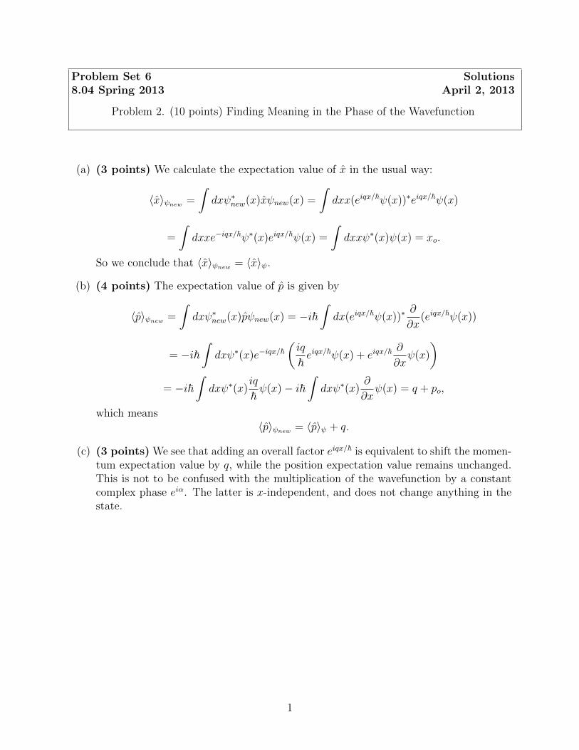
Problem Set 6 Solutions 8.04 Spring 2013 April 2, 2013

Problem 2. (10 points) Finding Meaning in the Phase of the Wavefunction

(a) (3 points) We calculate the expectation value of x in the usual way: iqx/nψ(x)) ∗ iqx/nψ(x)(ˆ = dxψ ∗ (x)ˆ (x) = dxx(e ex)ψnew new xψnew

dxxe−iqx/nψ ∗ (x)eiqx/nψ(x) == dxxψ ∗ (x)ψ(x) = xo.

So we conclude that (x)ψnew = (x)ψ.

(b) (4 points) The expectation value of p is given by iqx/nψ(x)) ∗ ∂ iqx/nψ(x))(ˆ = dxψ ∗ (x)pψnew(x) = −in dx(e (ep)ψnew new ∂x

−iqx/n iq iqx/nψ(x) + eiqx/n ∂ = −in dxψ ∗ (x)e

n e ψ(x)

∂x iq ∂

= −in dxψ ∗ (x)n ψ(x) − in dxψ ∗ (x) ψ(x) = q + po,

∂x

which means (ˆ = (p)ψ + q. p)ψnew

(c) (3 points) We see that adding an overall factor eiqx/n is equivalent to shift the momen­tum expectation value by q, while the position expectation value remains unchanged. This is not to be confused with the multiplication of the wavefunction by a constant complex phase eiα . The latter is x-independent, and does not change anything in the state.

1

Problem Set 6 Solutions 8.04 Spring 2013 April 2, 2013

Problem 3. (15 points) Relation between Wavefunction Phase and Probability Current

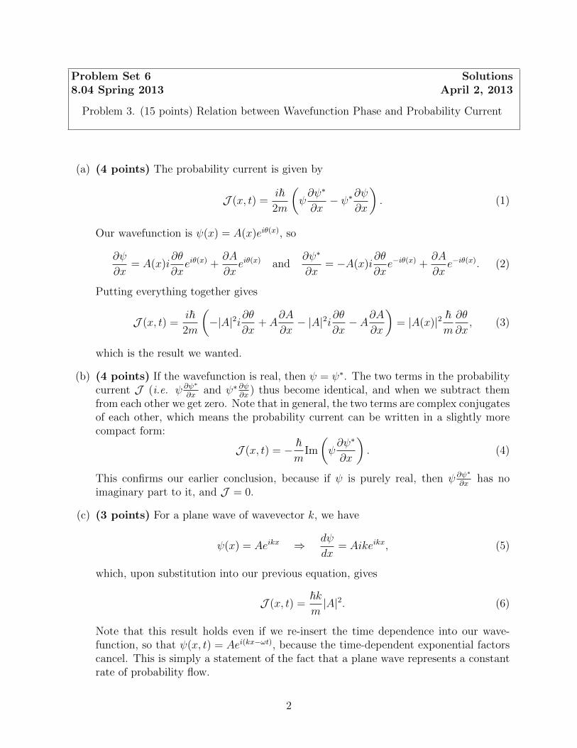
(a) (4 points) The probability current is given by

in ∂ψ∗ ∂ψ J (x, t) = ψ − ψ ∗ . (1)2m ∂x ∂x

iθ(x)Our wavefunction is ψ(x) = A(x)e , so

∂ψ ∂θ ∂A ∂ψ∗ ∂θ ∂A iθ(x) iθ(x) −iθ(x) −iθ(x)= A(x)i e + e and = −A(x)i e + e . (2)∂x ∂x ∂x ∂x ∂x ∂x

Putting everything together gives

in ∂θ ∂A ∂θ ∂A ∂θ J (x, t) = −|A|2i + A − |A|2i − A = |A(x)|2 n , (3)

2m ∂x ∂x ∂x ∂x m∂x

which is the result we wanted.

(b) (4 points) If the wavefunction is real, then ψ = ψ∗ . The two terms in the probability ψ ∂ψ

∗ current J (i.e. and ψ∗ ∂ψ ) thus become identical, and when we subtract them

∂x ∂x from each other we get zero. Note that in general, the two terms are complex conjugates of each other, which means the probability current can be written in a slightly more compact form:

n ∂ψ∗

J (x, t) = − Im ψ . (4) m ∂x

This confirms our earlier conclusion, because if ψ is purely real, then ψ ∂ψ∗ has no

∂x imaginary part to it, and J = 0.

(c) (3 points) For a plane wave of wavevector k, we have

ψ(x) = Aeikx ⇒ dψ

= Aikeikx , (5)dx

which, upon substitution into our previous equation, gives

nk J (x, t) = |A|2 . (6) m

Note that this result holds even if we re-insert the time dependence into our wave-function, so that ψ(x, t) = Aei(kx−ωt), because the time-dependent exponential factors cancel. This is simply a statement of the fact that a plane wave represents a constant rate of probability flow.

2

( )

( )

( )

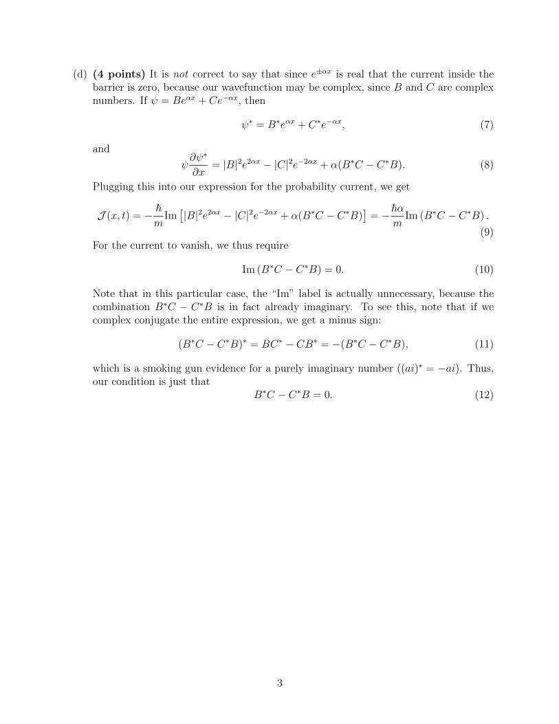
(d) (4 points) It is not correct to say that since e±αx is real that the current inside the barrier is zero, because our wavefunction may be complex, since B and C are complex numbers. If ψ = Beαx + Ce−αx, then

ψ ∗ αx −αx = B ∗ e + C ∗ e , (7)

and ∂ψ∗

ψ = |B|2 e 2αx − |C|2 e −2αx + α(B ∗ C − C ∗ B). (8)∂x

Plugging this into our expression for the probability current, we get

n nα J (x, t) = − Im |B|2 e 2αx − |C|2 e −2αx + α(B ∗ C − C ∗ B) = − Im (B ∗ C − C ∗ B) . m m

(9) For the current to vanish, we thus require

Im (B ∗ C − C ∗ B) = 0. (10)

Note that in this particular case, the “Im” label is actually unnecessary, because the combination B∗C − C∗B is in fact already imaginary. To see this, note that if we complex conjugate the entire expression, we get a minus sign:

(B ∗ C − C ∗ B) ∗ = BC ∗ − CB ∗ = −(B ∗ C − C ∗ B), (11)

which is a smoking gun evidence for a purely imaginary number ((ai)∗ = −ai). Thus, our condition is just that

B ∗ C − C ∗ B = 0. (12)

3

Problem Set 6 Solutions 8.04 Spring 2013 April 2, 2013

Problem 4. (15 points) Odd-parity Energy Eigenstates in the finite square well

(a) (3 points) The parameters which characterize this system are the length L, the energy V0 and the mass m. We can build a characteristic momentum by taking po

2 = 2mVo. Recalling that n has units of momentum times length (e.g., ΔxΔp ≥ n

2 ), we can trade this momentum for a second characteristic length Ro as,

n n Ro = = √ , (13)

po 2mVo

where we’ve kept the factor of 2 for later convenience. Ro is thus (up to factor of 2π) the quantum wavelength of a particle of mass m with energy Vo. We can now construct a dimensionless parameter,

L go = . (14)

Ro

Physically, the length Ro sets a lower limit on the size for the evanescent tails of bound −x/Rostates in the well: a state with energy E = −Vo would decay as e outside the

well; all bound states must decay more slowly. Meanwhile, the dimensionless constant go is a measure of how classical the well is – if go >> 1, the the evenescent tails are negligibly small and quantum effects can be generally ignored. Note that this obtains when the well is sufficiently deep and wide. We’ll come back to this in part (c) below.

(b) (6 points) The finite square well has potential −V0 for − L ≤ x ≤ L

V (x) = (15)0 for |x| > L.

We now proceed to solve the Schrodinger equation in the different regions. First we deal with |x| > L, where V = 0. This gives

n2 d2 n2 d2 d2ψ − + V ψ(x) = − ψ(x) = Eψ(x) ⇒ = κ2ψ, (16)2m dx2 2m dx2 dx2

√ where κ ≡ −2mE/n. We choose to write κ this way because we are searching for bound states, so E < 0 and κ > 0. The general solution to this equation is

ψ(x) = Ae−κx + Beκx . (17)

For x < −L, we must have A = 0, because otherwise ψ would diverge as x → −∞ and be unnormalizable. Similarly, for x > L we must have B = 0 to prevent a divergence as x → ∞. This means

Beκx for x < −L ψ(x) = (18)

Ae−κx for x > L.

4

( )

Now consider the region −L ≤ x ≤ L, where the Schrodinger equation takes the form

n2 d2 d2ψ − + V0 ψ(x) = Eψ(x) ⇒ = −l2ψ, (19)2m dx2 dx2

where l ≡ 2m(E + V0)/n. The differential equation is the same as that for a free particle, so the general solution is

ψ(x) = C sin(lx) + D cos(lx). (20)

In this problem we are searching for solutions with odd parity. The sine function is odd while the cosine function is even. We can therefore say that D = 0. Putting everything together, we have

ψ(x) =

⎧ ⎪⎨ ⎪⎩

Ae−κx for x > L

D sin(lx) for − L < x < L (21)

−Aeκx for x < −L, where we have taken advantage of the fact that we are dealing with odd-parity states to insist that the normalization constants on either side of the origin (e.g. the A’s) are the same. This allows to avoid having to deal with the x < 0 region separately. Our next step is to match boundary conditions. First we require that the wavefunction be continuous at x = L:

Ae−κL = D sin(lL).

We also require the derivative to be continuous there, which means

−Aκe−κL = Dl cos(lL).

(22)

(23)

Taking the ratio of these two equations gives

κ = −l cot(lL). (24)

Since l and κ contain only E, V0, and constant factors like n, what we have here is a transcendental equation for the permissible energies. At this point we non­dimensionalize by letting

L L√ L z ≡ 2m(E + V0), y ≡ −2mE, and go = 2mV0 (25)

n n nWith a little algebra, one can show that our transcendental equation thus becomes a pair of equations to be solved simultaneously:

y = −z cot z (26a) 2 2 2 go = y + z . (26b)

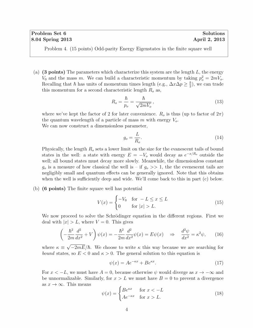
Given a value for go, these equations can be solved graphically. In the plot below, we show y = −z cot z in blue and go

2 = y2 + z2 in red, with go set to 10. A solution exists whenever the curves intersect. In the example shown below, for example, we see that for the odd-parity states we are considering in this problem, there exist three bound states. Once the values of z at the intersections have been found, one can go back to the definition of z shown above to calculate the bound state energies E.

5

( )

2 4 6 8 10 12z

!20

!10

10

20

y

(c) (4 points) If go is very large, then the intersections occur very close to the locations of the discontinuities in the cotangent function, that is, at multiples of π. This can be seen in the plot below, where we have set go = 100.

10 20 30 40z

!100

100

200

y

Substituting this back into our definition of z, we get

(n + 1)2π2n2

En − (−V0) ≈ , (27)2m(2L)2

where n is odd. The left hand side is the energy of the state above the bottom of the well (which is at energy −V0). Referring back to Problem set 4, we see that the right hand side precisely the energy of the nth energy eigenstate for an infinite potential well of width 2L. This makes sense — if go is large, then we have a very deep well, one which is an excellent approximation to an infinite well. Note that we only get the odd energies here, because we have only considered solutions with odd parity. As go is decreased, the number of bound states decreases. In the plot below, we show a variety of go’s.

2 4 6 8 10z

!5

5

10

y

6

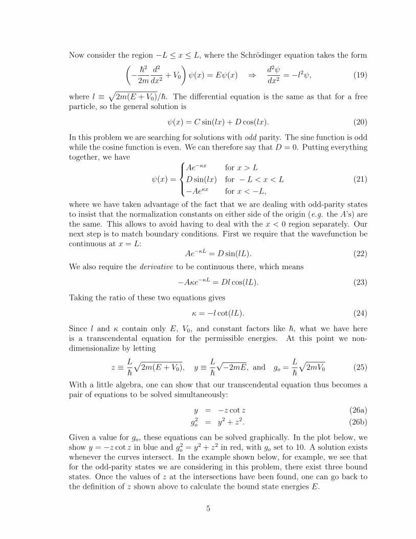
As go decreases, the red curves “sweep left”, and eventually we no longer have any bound states. This occurs when go is so small that the red curves hit the horizontal axis while the blue curve is still negative. Since the blue curve crosses the axis at z = π/2, the condition for a bound state to exist is

π π go ≥

2 ⇒ L ≥

2 Ro. (28)

The latter inequality tells us that, holding Ro fixed, in order to have an odd bound state L has to be large, and conversely, holding L fixed, Ro has to be small, i.e. the square well has to be deeper than a certain value. Remember that, as we saw in class, there is always at least one even bound state.

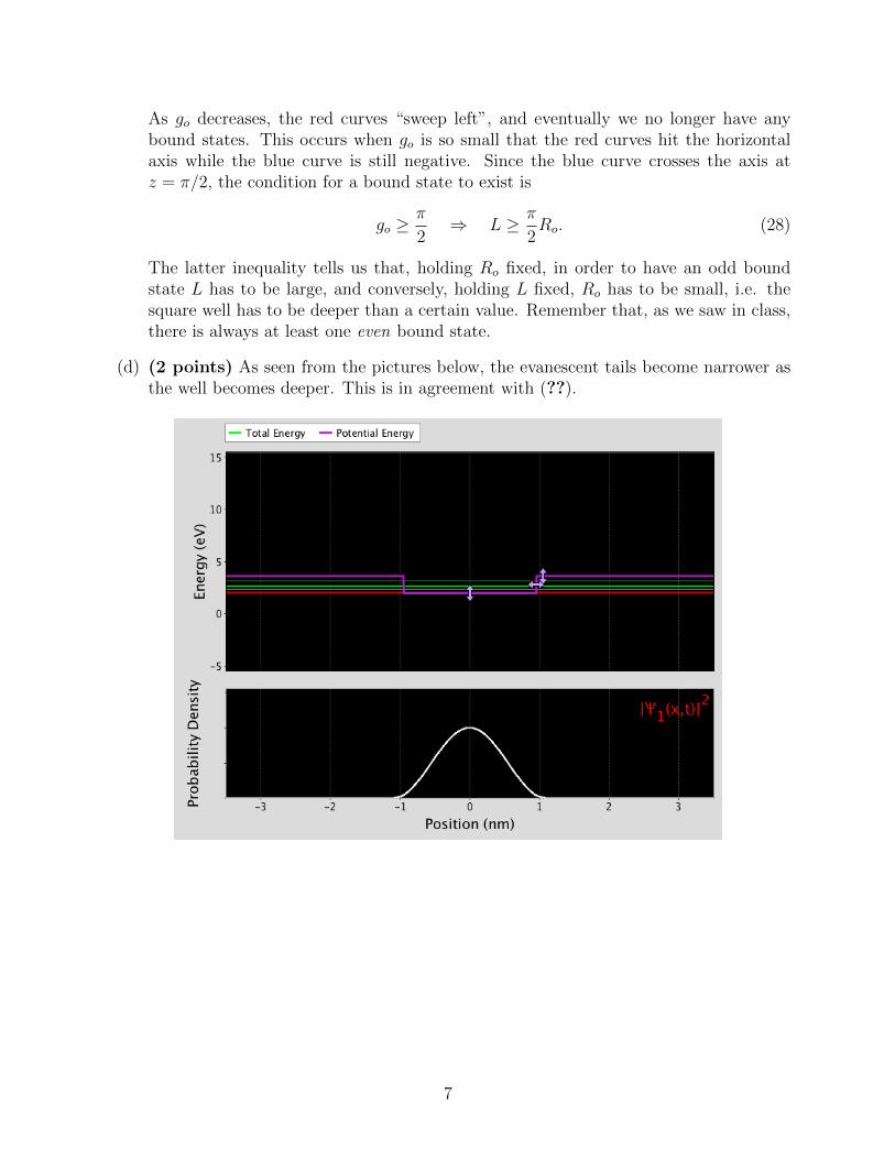
(d) (2 points) As seen from the pictures below, the evanescent tails become narrower as the well becomes deeper. This is in agreement with (??).

7

8

Problem Set 6 Solutions 8.04 Spring 2013 April 2, 2013

Problem 5. (35 points) Quantum Glue

(a) (10 points) For bound states, where E < 0, the wavefunction takes the following form:

ψ(x) =

⎧ ⎪⎨ ⎪⎩

Aeκx for −∞ < x < −L

Ceκx + De−κx for − L < x < L (29)

Fe−κx for L < x < ∞, √

where κ ≡ −2n mE , and we have excluded the decaying exponential solution in the

leftmost region and the growing exponential solution in the rightmost region in order to ensure that our wavefunction is normalizable. Because our potential is even, we can make our life simpler by remembering that the energy eigenfunctions must be either even or odd: ⎧ ⎪⎨ ⎪⎩

Aeκx for −∞ < x < −L

B cosh κx for − L < x < L (30)

Ae−κx for L < x < ∞,

ψeven(x) =

and ⎧ ⎪⎨ ⎪⎩

Ceκx for −∞ < x < −L

D sinh κx for − L < x < L (31)

−Ce−κx for L < x < ∞.

ψodd(x) =

(Recall that the hyperbolic cosine and hyperbolic sine functions are the even and odd combinations respectively of real exponentials). First let us deal with the even solutions. Continuity of the wavefunction requires

B cosh κL = Ae−κL . (32)

The jump condition is dψ dx

− dψ dx

= − 2mW0

n2 ψ(a), (33)

−a+ a

so we have

−κAe−κL − Bκ sinh κL = − 2mW0

Ae−κL . (34)n2

Eliminating A and B from these equations gives

2mW0tanh κL =

n2κ − 1 . (35)

√

Since κ ≡ −2mE , this is an implicit equation for the bound state energies. We can n non-dimensionalize the equation by letting ξ ≡ κL and g0 ≡ mLW0 : n2

ξ + ξ tanh ξ = 2g0 (36)

9

( )

As for the odd solutions, continuity requires

D sinh κL = −Ce−κL , (37)

while the jump in the slope tells us that

2mW0Cκe−κL − Dκ cosh κL =

n2 Ce−κL (38)

Eliminating C and D gives

tanh κL = 2mW0

n2κ − 1

−1

⇒ ξ + ξ coth ξ = 2g0. (39)

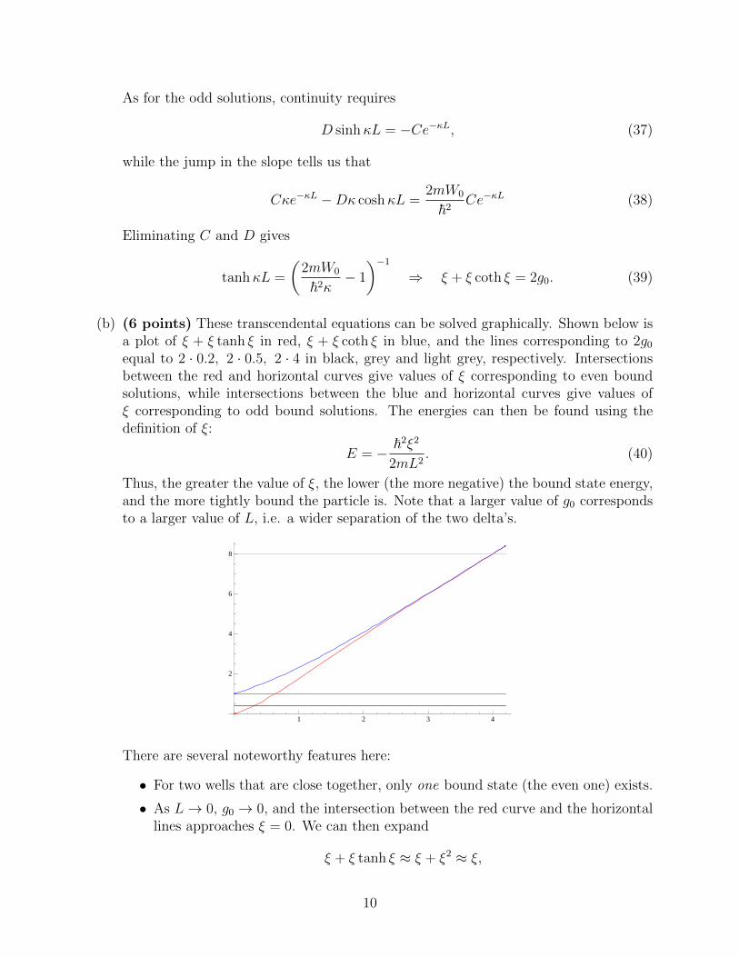
(b) (6 points) These transcendental equations can be solved graphically. Shown below is a plot of ξ + ξ tanh ξ in red, ξ + ξ coth ξ in blue, and the lines corresponding to 2g0

equal to 2 · 0.2, 2 · 0.5, 2 · 4 in black, grey and light grey, respectively. Intersections between the red and horizontal curves give values of ξ corresponding to even bound solutions, while intersections between the blue and horizontal curves give values of ξ corresponding to odd bound solutions. The energies can then be found using the definition of ξ:

n2ξ2

E = − . (40)2mL2

Thus, the greater the value of ξ, the lower (the more negative) the bound state energy, and the more tightly bound the particle is. Note that a larger value of g0 corresponds to a larger value of L, i.e. a wider separation of the two delta’s.

1 2 3 4

2

4

6

8

There are several noteworthy features here:

• For two wells that are close together, only one bound state (the even one) exists.

• As L → 0, g0 → 0, and the intersection between the red curve and the horizontal lines approaches ξ = 0. We can then expand

ξ + ξ tanh ξ ≈ ξ + ξ2 ≈ ξ,

10

( )

so that the corresponding trascendental equation simplifies to

ξ ξ = 2g0 ⇒ = 2.

g0

Plugging this value into our formula for the energy, we see that

m(2W0)2

Eclose = − , (41)2n2

which is precisely the ground state energy for a single delta function well of strength 2W0! Physically, this is because the wells are so close together that they effectively look like one well.

• As the separation between the wells is increased (i.e. as L, and therefore g0 is increased), we eventually get to a point where there are two bound states.

• When there are two bound states, the even bound state always has a higher value of ξ than the odd bound state. From Equation 40, we thus see the even state is always more tightly bound than the odd state. This makes sense because we know the ground state cannot have any nodes by the node theorem, so it must be even.

• For widely separated wells, g0 is large and both the even and odd solutions ap­proach ξ = g0. Indeed, it’s easy to see from the plot that large g0 gives large values of ξ at the intersections, so we can approximate tanh ξ, coth ξ ≈ 1, and both the trascendental equations become

2ξ = 2g0.

Correspondingly, the energies of the two states are almost degenerate, with energy close to

mW02

Efar = − , (42)2n2

which is the ground state energy of a single delta function potential. Physically, this is because two widely-separated wells effectively operate as independent single wells.

• The separation L at which the second bound state appears (i.e. when we get the first odd bound state) can be computed by the following technique. As we √

2mEincrease g0 (and therefore L), we eventually get to a point where κ = n2

is approximately zero (the odd “bound-state-in-waiting” is barely bound). The wavefunction may thus be Taylor expanded in κ:

ψodd(x) =

⎧ ⎪⎨ ⎪⎩

C(1 + κx) for −∞ < x < −L

Dκx for − L < x < L (43)

−C(1 − κx) for L < x < ∞.

The continuity and jump conditions are therefore

2mW0DκL = −C(1 − κL) and Cκ − Dκ = − DκL. (44)

n2

11

Solving these gives (1 − 2g0)(κL − 1) = κL. (45)

We wish to take the limit κ → 0, because we want to find the g0 (and therefore L) when the second bound state first appears. Doing so tells us that

crit 1 n2

g0 = ⇒ Lcrit = . (46)2 2mW0

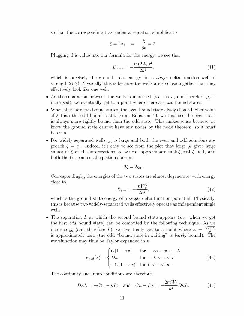
(c) (5 points) From part (b) we know that g0 = 0.1 gives a single even bound state:

-20 -10 10 20xL

0.4

0.6

0.8

1.0

Ψ ´Ñ

2

m W0

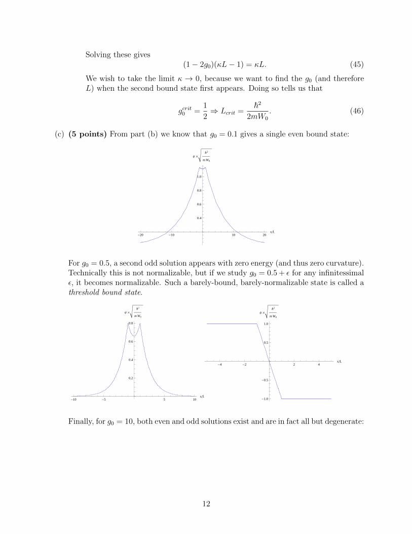
For g0 = 0.5, a second odd solution appears with zero energy (and thus zero curvature). Technically this is not normalizable, but if we study g0 = 0.5 + f for any infinitessimal f, it becomes normalizable. Such a barely-bound, barely-normalizable state is called a threshold bound state.

-10 -5 5 10xL

0.2

0.4

0.6

0.8

Ψ ´Ñ

2

m W0

-4 -2 2 4xL

-1.0

-0.5

0.5

1.0

Ψ ´Ñ

2

m W0

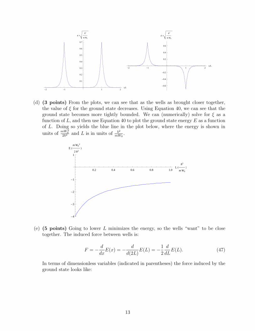
Finally, for g0 = 10, both even and odd solutions exist and are in fact all but degenerate:

12

-2 -1 1 2xL

0.1

0.2

0.3

0.4

0.5

0.6

0.7

Ψ ´Ñ

2

m W0

-2 -1 1 2xL

-0.6

-0.4

-0.2

0.2

0.4

0.6

Ψ ´Ñ

2

m W0

(d) (3 points) From the plots, we can see that as the wells as brought closer together, the value of ξ for the ground state decreases. Using Equation 40, we can see that the ground state becomes more tightly bounded. We can (numerically) solve for ξ as a function of L, and then use Equation 40 to plot the ground state energy E as a function of L. Doing so yields the blue line in the plot below, where the energy is shown in

mW 2 n2 units of 0 and L is in units of .

2n2 mW0

0.2 0.4 0.6 0.8 1.0L

Ñ2

m W0

-4

-3

-2

-1

1

E m W0

2

2 Ñ2

(e) (5 points) Going to lower L minimizes the energy, so the wells “want” to be close together. The induced force between wells is:

d d 1 d F = − E(x) = − E(L) = − E(L). (47)

dx d(2L) 2 dL

In terms of dimensionless variables (indicated in parentheses) the force induced by the ground state looks like:

13

0.2 0.4 0.6 0.8 1.0L

Ñ2

m W0

-140

-120

-100

-80

-60

-40

-20

F m2 W0

3

2 Ñ4

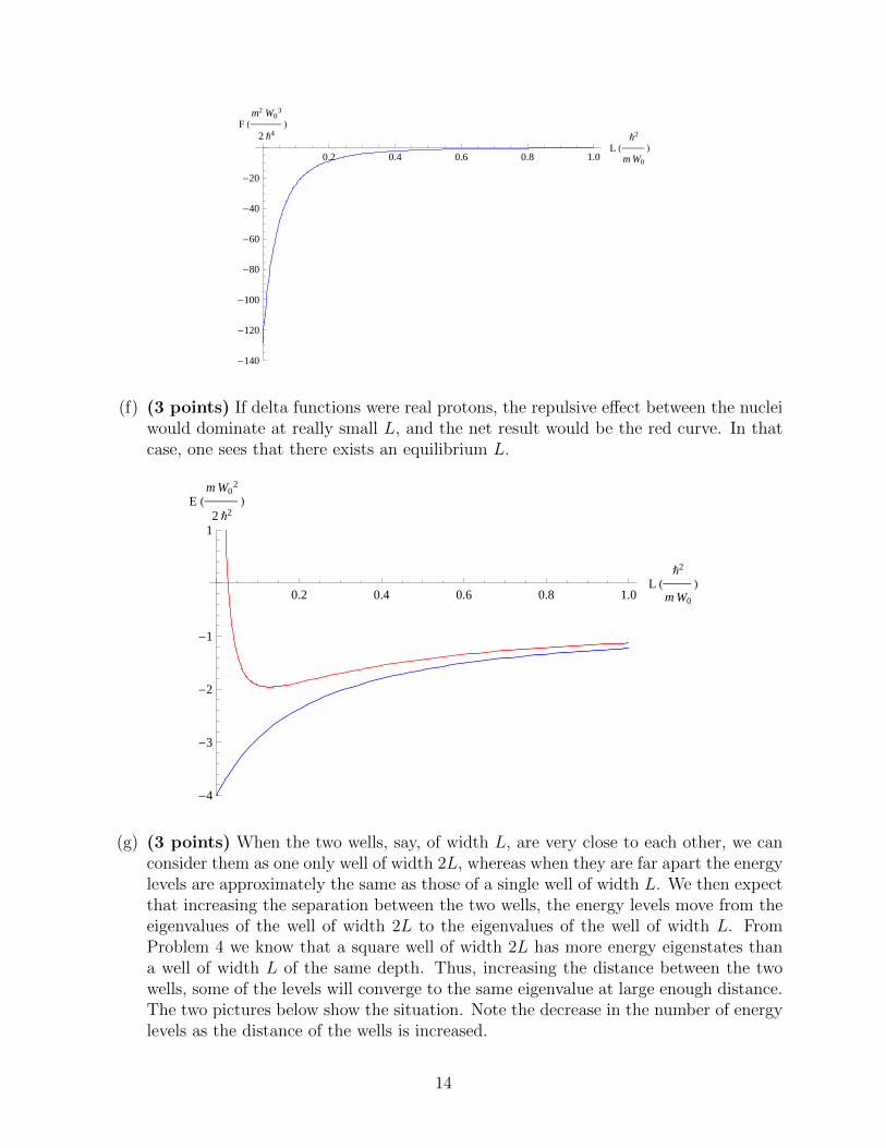
(f) (3 points) If delta functions were real protons, the repulsive effect between the nuclei would dominate at really small L, and the net result would be the red curve. In that case, one sees that there exists an equilibrium L.

0.2 0.4 0.6 0.8 1.0L

Ñ2

m W0

-4

-3

-2

-1

1

E m W0

2

2 Ñ2

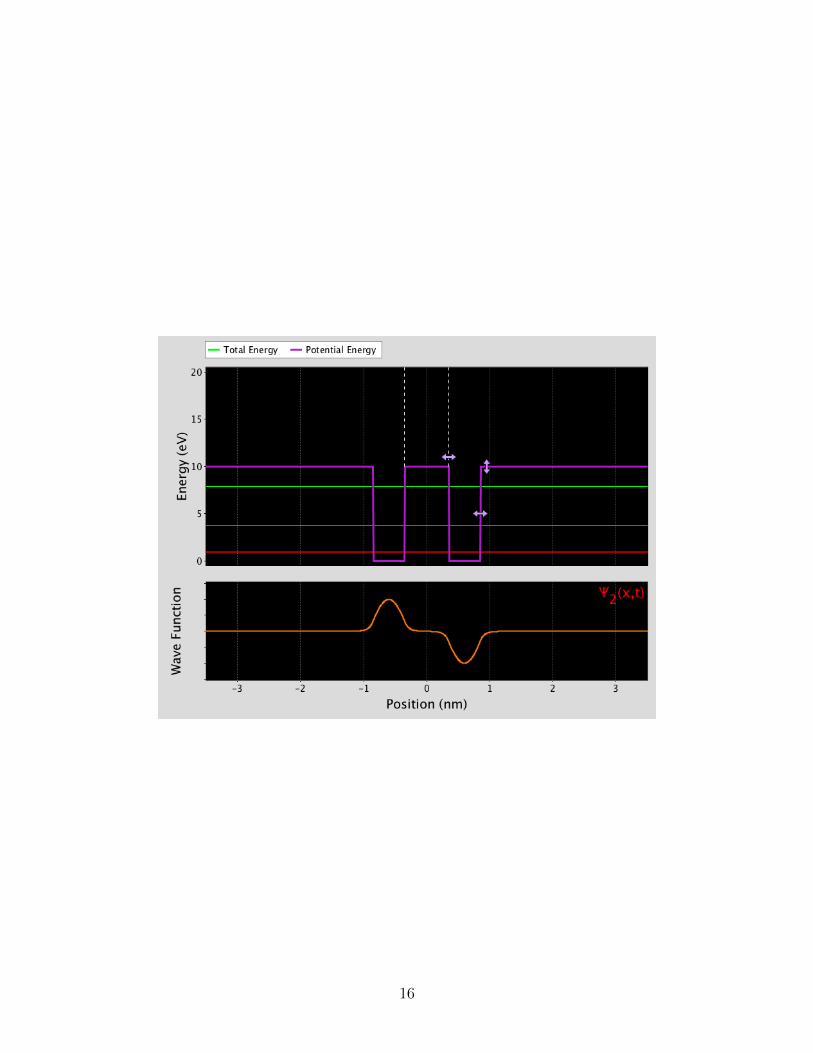
(g) (3 points) When the two wells, say, of width L, are very close to each other, we can consider them as one only well of width 2L, whereas when they are far apart the energy levels are approximately the same as those of a single well of width L. We then expect that increasing the separation between the two wells, the energy levels move from the eigenvalues of the well of width 2L to the eigenvalues of the well of width L. From Problem 4 we know that a square well of width 2L has more energy eigenstates than a well of width L of the same depth. Thus, increasing the distance between the two wells, some of the levels will converge to the same eigenvalue at large enough distance. The two pictures below show the situation. Note the decrease in the number of energy levels as the distance of the wells is increased.

14

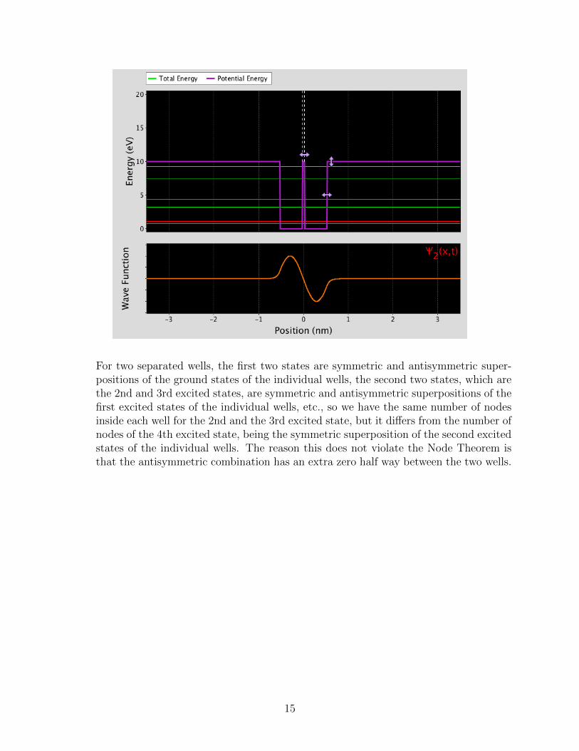
For two separated wells, the first two states are symmetric and antisymmetric super­positions of the ground states of the individual wells, the second two states, which are the 2nd and 3rd excited states, are symmetric and antisymmetric superpositions of the first excited states of the individual wells, etc., so we have the same number of nodes inside each well for the 2nd and the 3rd excited state, but it differs from the number of nodes of the 4th excited state, being the symmetric superposition of the second excited states of the individual wells. The reason this does not violate the Node Theorem is that the antisymmetric combination has an extra zero half way between the two wells.

15

16

Problem Set 6 Solutions 8.04 Spring 2013 April 2, 2013

Problem 6. (15 points) Further Facts about Hermitian Operators and Commutators

(a) (2 points)

Note the following useful property:

∗

(f |g) ∗ ≡ f ∗ gdx = g ∗ fdx = (g|f). (48)

But we already know that: (f | ˆ g) = ( ˆ (49)A† Af |g),

which combined with Eq. 48 gives us the answer:

A†(f | ˆ g) = ( ˆ Af) ∗ . (50)Af |g) = (g| ˆ

(b) (2 points) To find the adjoint of in, it is useful to go back to writing out the integrals ˆthat define the adjoint. If we let A = in we have

f ∗ ingdx = (−inf) ∗ gdx, (51)

where we have simply used the definition of complex conjugation. So we see that the ˆadjoint of A = in must be

A† = −in. (52)

(c) (2 points) First we use the definition of the adjoint:

(f |( ˆ g) = ( ˆBf |g), (53)AB)† A ˆ

where we thought of AB as a single operator and moved it to the left as one “package”. ˆ ˆThe trick now is to treat A as an operator acting on the state Bf and to use the

ˆdefinition of the adjoint to “bring A back”:

A†(A( ˆ Bf | ˆ g). (54)Bf)|g) = ( ˆ

Now we do the same for B, treating it as an operator that acts on the state A†g:

A†(Bfˆ |A† g) = (f |B† ˆ g). (55)

Putting everything together, we see that in general,

(AB)† = B†A† . (56)

17

(∫ ) ∫

∫ ∫

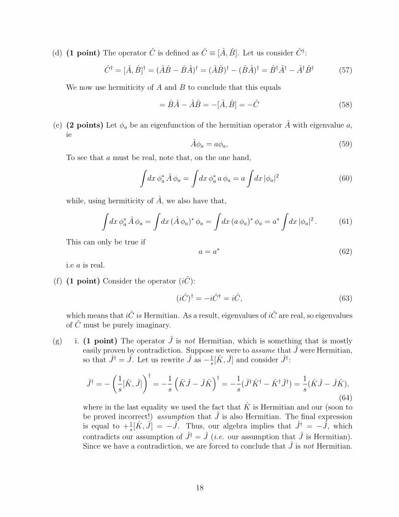
ˆ C ≡ [ ˆ C†:(d) (1 point) The operator C is defined as A, B]. Let us consider ˆ

C† = [ A,ˆ B]† = ( AB − BA)† = ( AB)† − (BA)† = B†A† − A†B† (57)

We now use hermiticity of A and B to conclude that this equals

= B ˆ A ˆ = −[ ˆ B] = − ˆ (58)ˆA − ˆB A, ˆ C

ˆ(e) (2 points) Let φa be an eigenfunction of the hermitian operator A with eigenvalue a, ie

ˆAφa = aφa, (59)

To see that a must be real, note that, on the one hand,

ˆ |2dx φ ∗ a Aφa = dx φ a

∗ a φa = a dx |φa (60)

ˆwhile, using hermiticity of A, we also have that,

dx φ ∗ Aφa = dx ( ˆ ) ∗ φa = dx (a φa = a dx |φa|2 . (61)a ˆ Aφa ) ∗ φa

∗

This can only be true if a = a ∗ (62)

i.e a is real.

(f) (1 point) Consider the operator (iC):

(iC)† = −iC† C, = i ˆ (63)

which means that iC is Hermitian. As a result, eigenvalues of iC are real, so eigenvalues ˆof C must be purely imaginary.

ˆ(g) i. (1 point) The operator J is not Hermitian, which is something that is mostly easily proven by contradiction. Suppose we were to assume that J were Hermitian,

ˆ ˆ [ ˆso that J† = J . Let us rewrite J as −1 s K, J ] and consider J†:

† †1 1 1 1 [ ˆ J ] ˆJ − ˆ ( ˆ K† − ˆ J†) = K ˆ J ˆJ† = − K, ˆ = − K ˆ JK = − J† ˆ K† ˆ ( ˆJ − ˆK), s s s s

(64) ˆwhere in the last equality we used the fact that K is Hermitian and our (soon to

ˆbe proved incorrect!) assumption that J is also Hermitian. The final expression is equal to +1

s [ˆ J ] = − ˆ Thus, our algebra implies that J† = − ˆ which K, ˆ J . ˆ J ,

J† ˆ ˆcontradicts our assumption of = J (i.e. our assumption that J is Hermitian). Since we have a contradiction, we are forced to conclude that J is not Hermitian.

18

∫ ∫ ∫

∫ ∫ ∫ ∫

( )

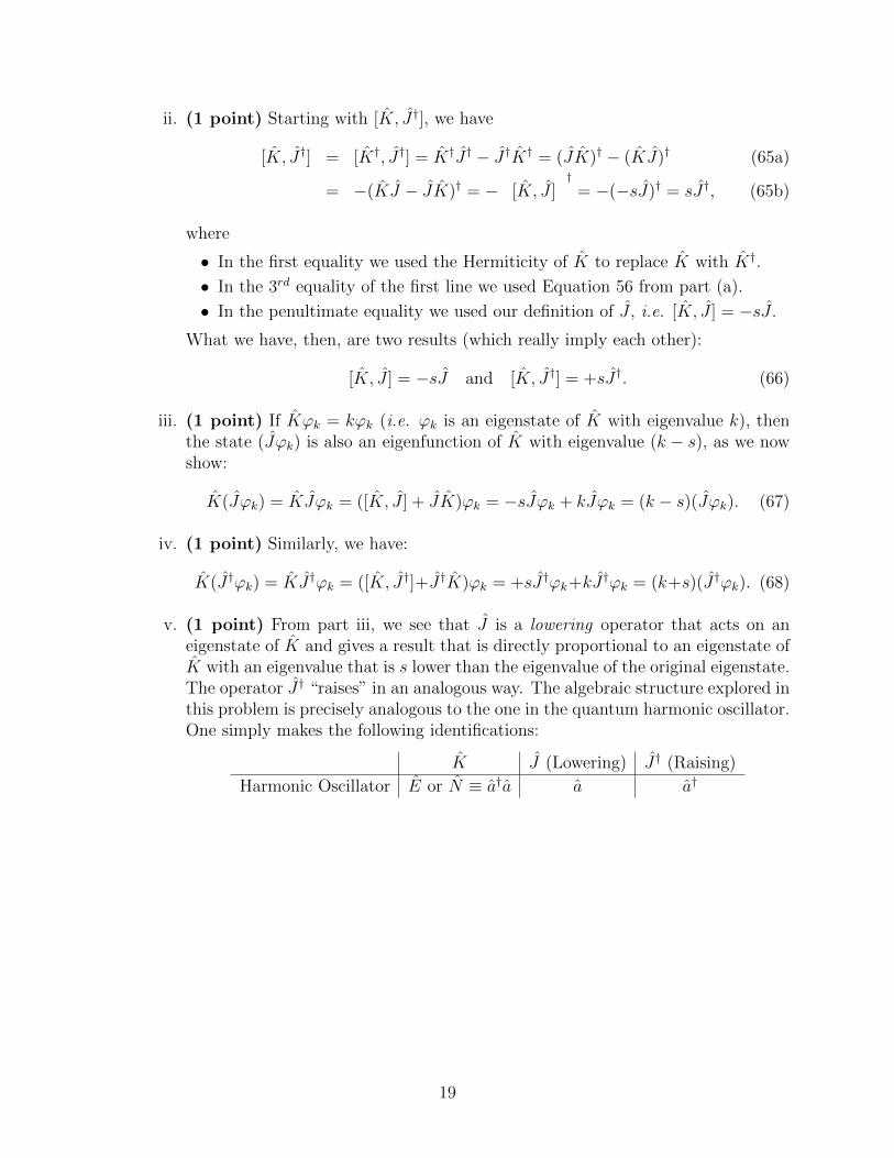
ii. (1 point) Starting with [ ˆ J†], we have K, ˆ

[ ˆ J†] [K† , ˆ K†J† − J† ˆ J ˆ K ˆ (65a)K, ˆ = J†] = ˆ K† = ( ˆK)† − ( ˆJ)†

† = −( ˆJ − ˆK)† = − [ ˆ J ] = −(−sJ)† = sJ† ,K ˆ J ˆ K, ˆ (65b)

where ˆ ˆ K†• In the first equality we used the Hermiticity of K to replace K with .

• In the 3rd equality of the first line we used Equation 56 from part (a).

• In the penultimate equality we used our definition of J , i.e. [ ˆ J ] = −sJ .K, ˆ

What we have, then, are two results (which really imply each other):

[K, ˆ J ] = −sJ and K, ˆ J † . (66)[ ˆ J†] = +s

ˆ ˆiii. (1 point) If Kϕk = kϕk (i.e. ϕk is an eigenstate of K with eigenvalue k), then the state ( ˆ K with eigenvalue (k − s), as we now Jϕk) is also an eigenfunction of show:

K(Jϕˆk) = KJϕˆ k = ([ K, ˆ ˆ JK)ϕk = −sJϕˆ k + k ˆ Jϕk). (67)J ] + Jϕk = (k − s)( ˆ

iv. (1 point) Similarly, we have:

K(J†ϕk) = KJ†ϕk = ([ ˆ J†]+ J† ˆ J†ϕk +kJ†ϕk = (k+s)(J†ϕk). (68)K, ˆ K)ϕk = +s

ˆv. (1 point) From part iii, we see that J is a lowering operator that acts on an ˆeigenstate of K and gives a result that is directly proportional to an eigenstate of

K with an eigenvalue that is s lower than the eigenvalue of the original eigenstate. The operator J† “raises” in an analogous way. The algebraic structure explored in this problem is precisely analogous to the one in the quantum harmonic oscillator. One simply makes the following identifications:

K J (Lowering) J† (Raising) Harmonic Oscillator E or N ≡ a†a a a†

19

MIT OpenCourseWarehttp://ocw.mit.edu

8.04 Quantum Physics ISpring 2013

For information about citing these materials or our Terms of Use, visit: http://ocw.mit.edu/terms.