SVD

Bin An; Chunye Wang

2

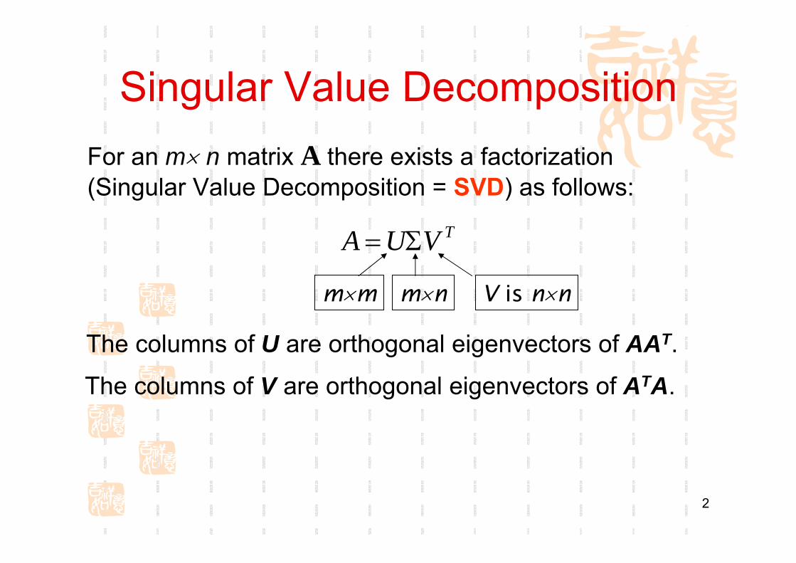
Singular Value Decomposition

TVUA Σ=

m×m m×n V is n×n

For an m× n matrix A there exists a factorization(Singular Value Decomposition = SVD) as follows:

The columns of U are orthogonal eigenvectors of AAT.

The columns of V are orthogonal eigenvectors of ATA.

3

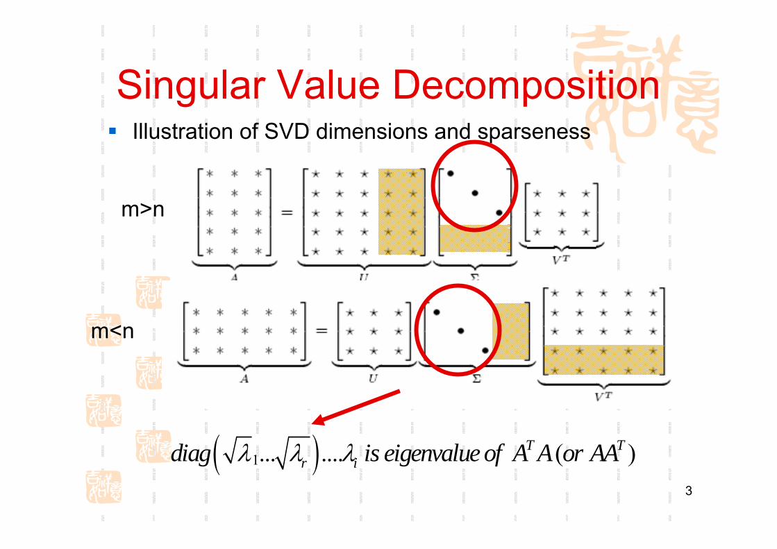
Singular Value DecompositionIllustration of SVD dimensions and sparseness

m>n

m<n

( )1... .... ( )T Tr idiag is eigenvalueof A A or AAλ λ λ

4

SVD example1 0.52 1.1

10 4.911 5.6

A

⎡ ⎤⎢ ⎥⎢ ⎥=⎢ ⎥⎢ ⎥⎣ ⎦

Matlab: [U S V]=svd(A)

-0.0665 0.0080 -0.7239 -0.6866 16.8168 0 -0.1356 -0.5652 0.5633 -0.5873 -0.6622 0.6614 0.2759 -0.2190 -0.7340 -0.4930 -0.2874 0.3683

⎡ ⎤⎢ ⎥⎢ ⎥⎢ ⎥⎢ ⎥⎣ ⎦

0 0.1538 -0.8939 0.4482 0 0 -0.4482 -0.8939

0 0

⎡ ⎤⎢ ⎥ ⎡ ⎤⎢ ⎥ ⎢ ⎥⎢ ⎥ ⎣ ⎦⎢ ⎥⎣ ⎦

1

2

16.81680.1538

λλ

==

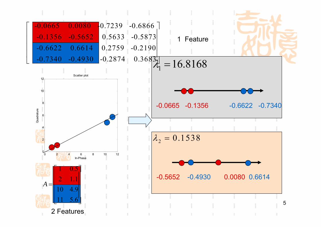
5

1 16.8168λ =

0 2 4 6 8 10 120

2

4

6

8

10

12

Qua

drat

ure

In-Phase

Scatter plot

-0.0665 -0.1356 -0.6622 -0.7340

1 16.8168λ =

-0.5652 -0.4930 0.0080 0.6614

2 0.1538λ =

-0.0665 0.0080 -0.7239 -0.6866 -0.1356 -0.5652 0.5633 -0.5873 -0.6622 0.6614 0.2759 -0.2190 -0.7340 -0.4930 -0.2874 0.3683

⎡ ⎤⎢ ⎥⎢ ⎥⎢ ⎥⎢ ⎥⎣ ⎦

2 Features

1 Feature

1 0.52 1.1

10 4.911 5.6

A

⎡ ⎤⎢ ⎥⎢ ⎥=⎢ ⎥⎢ ⎥⎣ ⎦

Probability Boot camp

Bin An; Chunye Wang

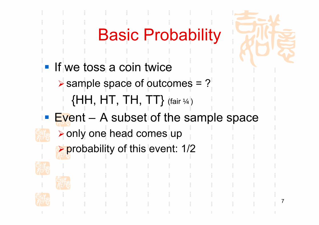
7

Basic Probability

If we toss a coin twice sample space of outcomes = ?{HH, HT, TH, TT} (fair ¼)

Event – A subset of the sample spaceonly one head comes upprobability of this event: 1/2

8

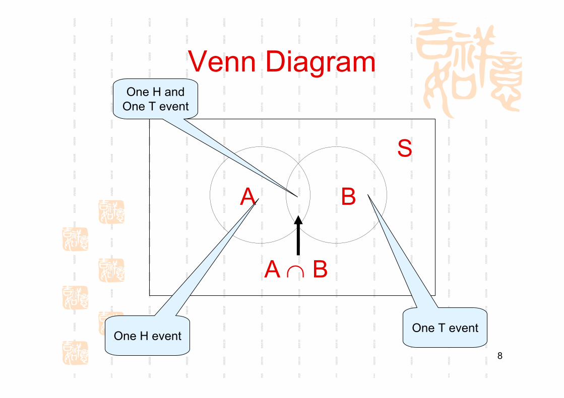
Venn Diagram

A B

A ∩ B

S

One H eventOne T event

One H and One T event

9

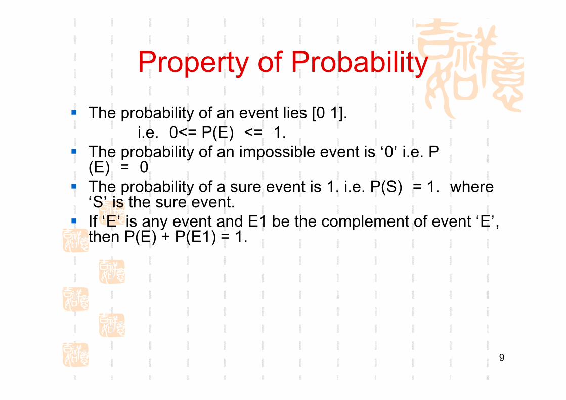
Property of ProbabilityThe probability of an event lies [0 1].

i.e. 0<= P(E) <= 1.The probability of an impossible event is ‘0’ i.e. P (E) = 0The probability of a sure event is 1. i.e. P(S) = 1. where ‘S’ is the sure event.If ‘E’ is any event and E1 be the complement of event ‘E’, then P(E) + P(E1) = 1.

10

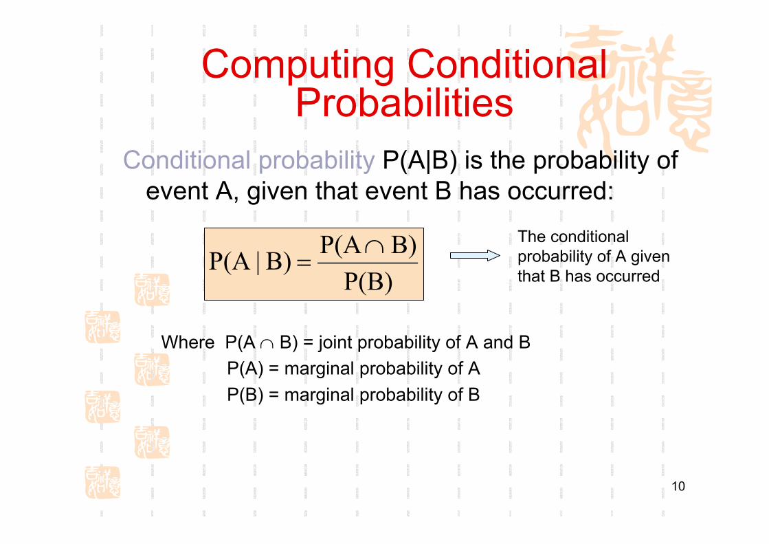
Computing Conditional Probabilities

Conditional probability P(A|B) is the probability of event A, given that event B has occurred:

P(B)B)P(AB)|P(A ∩

=

Where P(A ∩ B) = joint probability of A and BP(A) = marginal probability of AP(B) = marginal probability of B

The conditional probability of A given that B has occurred

11

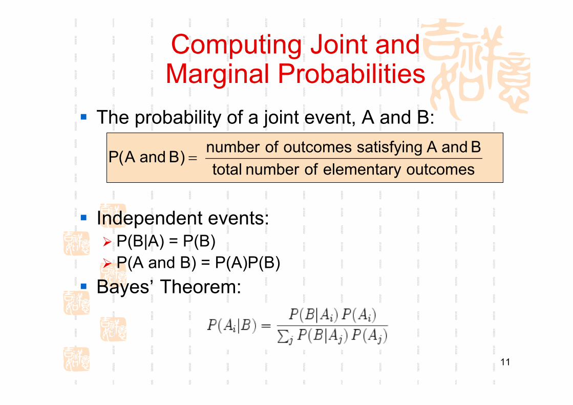
Computing Joint and Marginal Probabilities

The probability of a joint event, A and B:

Independent events:P(B|A) = P(B)P(A and B) = P(A)P(B)

Bayes’ Theorem:

outcomeselementaryofnumbertotalBandAsatisfyingoutcomesofnumber)BandA(P =

12

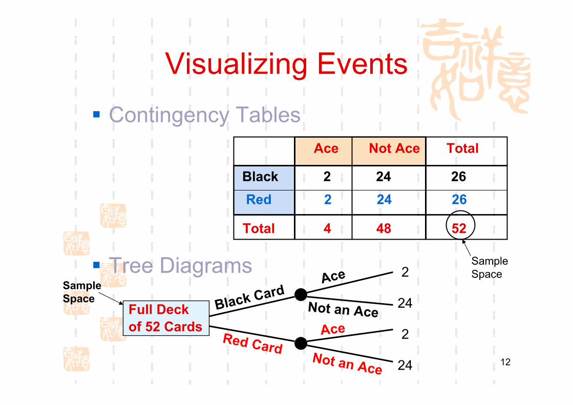
Visualizing EventsContingency Tables

Tree Diagrams

Red 2 24 26Black 2 24 26

Total 4 48 52

Ace Not Ace Total

Full Deck of 52 Cards

Red Card

Black Card

Not an Ace

Ace

AceNot an Ace

Sample Space

Sample Space2

24

2

24

13

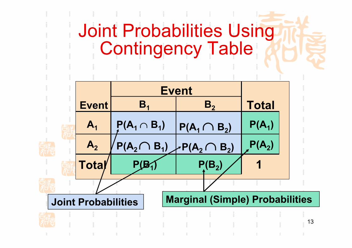
P(A1 ∩ B2) P(A1)

TotalEvent

Joint Probabilities Using Contingency Table

P(A2 ∩ B1)

P(A1 ∩ B1)

Event

Total 1

Joint Probabilities Marginal (Simple) Probabilities

A1

A2

B1 B2

P(B1) P(B2)

P(A2 ∩ B2) P(A2)

14

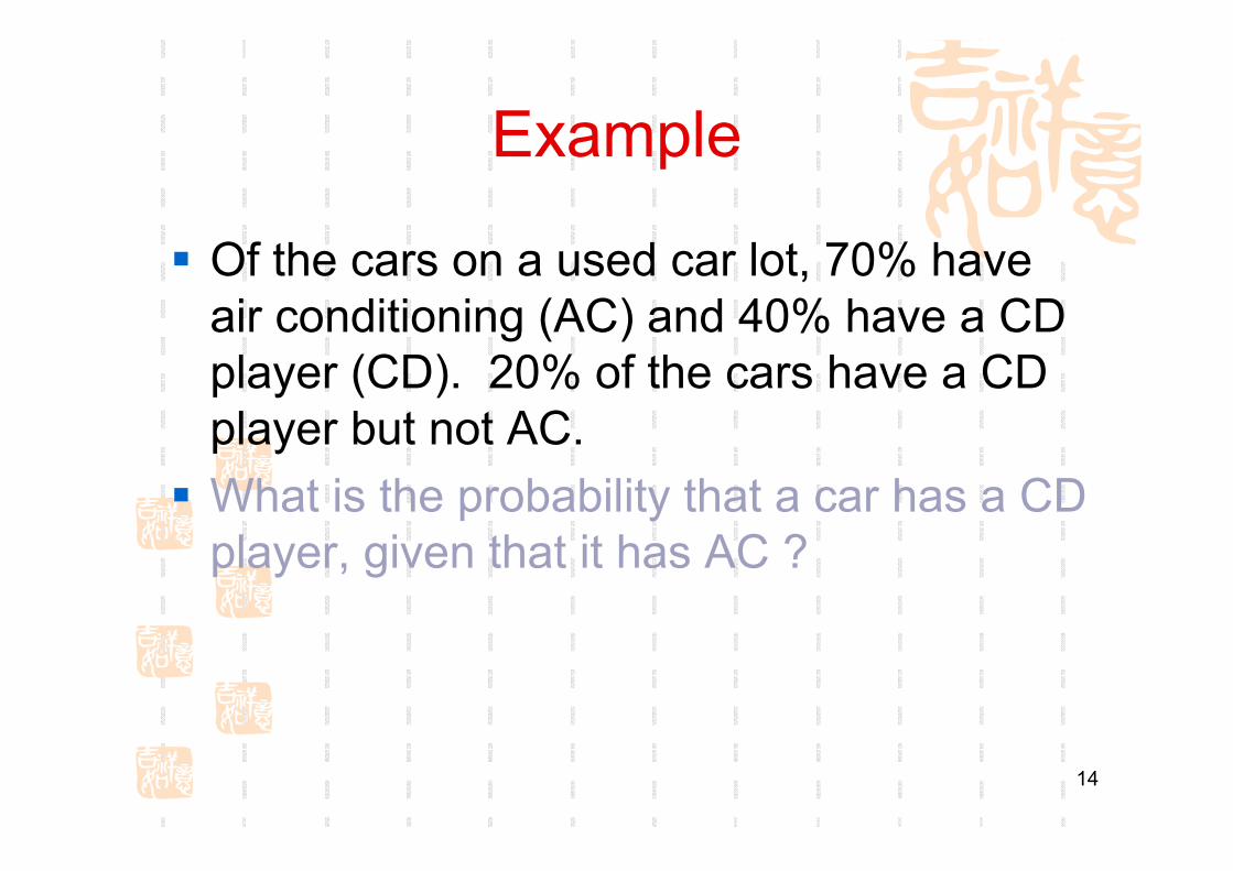
Example

Of the cars on a used car lot, 70% have air conditioning (AC) and 40% have a CD player (CD). 20% of the cars have a CD player but not AC.What is the probability that a car has a CD player, given that it has AC ?

15

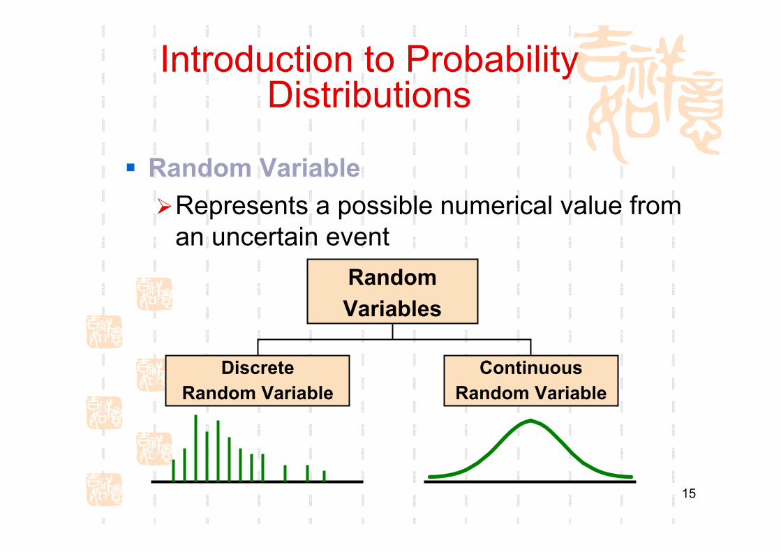
Introduction to Probability Distributions

Random VariableRepresents a possible numerical value from an uncertain event

Random Variables

Discrete Random Variable

ContinuousRandom Variable

16

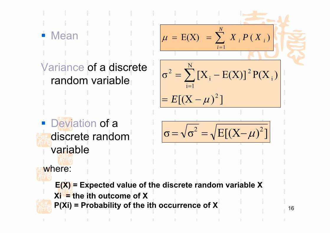
Mean

Variance of a discrete random variable

Deviation of a discrete random variable

])[(X

)P(XE(X)][Xσ

2

N

1ii

2i

2

μ−=

−= ∑=

E

])E[(Xσσ 22 μ−==

∑=

==N

iii XPX

1)( E(X) μ

where:

E(X) = Expected value of the discrete random variable XXi = the ith outcome of XP(Xi) = Probability of the ith occurrence of X

17

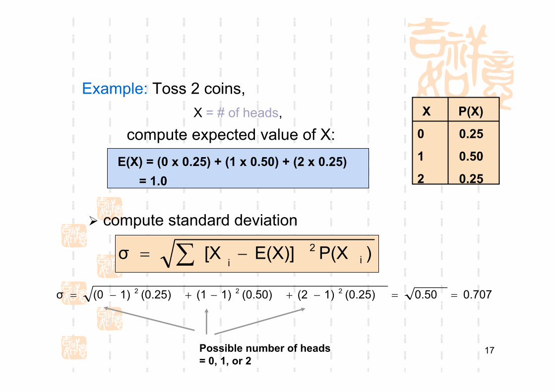
Example: Toss 2 coins, X = # of heads,

compute expected value of X:E(X) = (0 x 0.25) + (1 x 0.50) + (2 x 0.25)

= 1.0

X P(X)

0 0.25

1 0.50

2 0.25

compute standard deviation

)P(XE(X)][Xσ i2

i−= ∑

0.7070.50(0.25)1)(2(0.50)1)(1(0.25)1)(0σ 222 ==−+−+−=

Possible number of heads = 0, 1, or 2

18

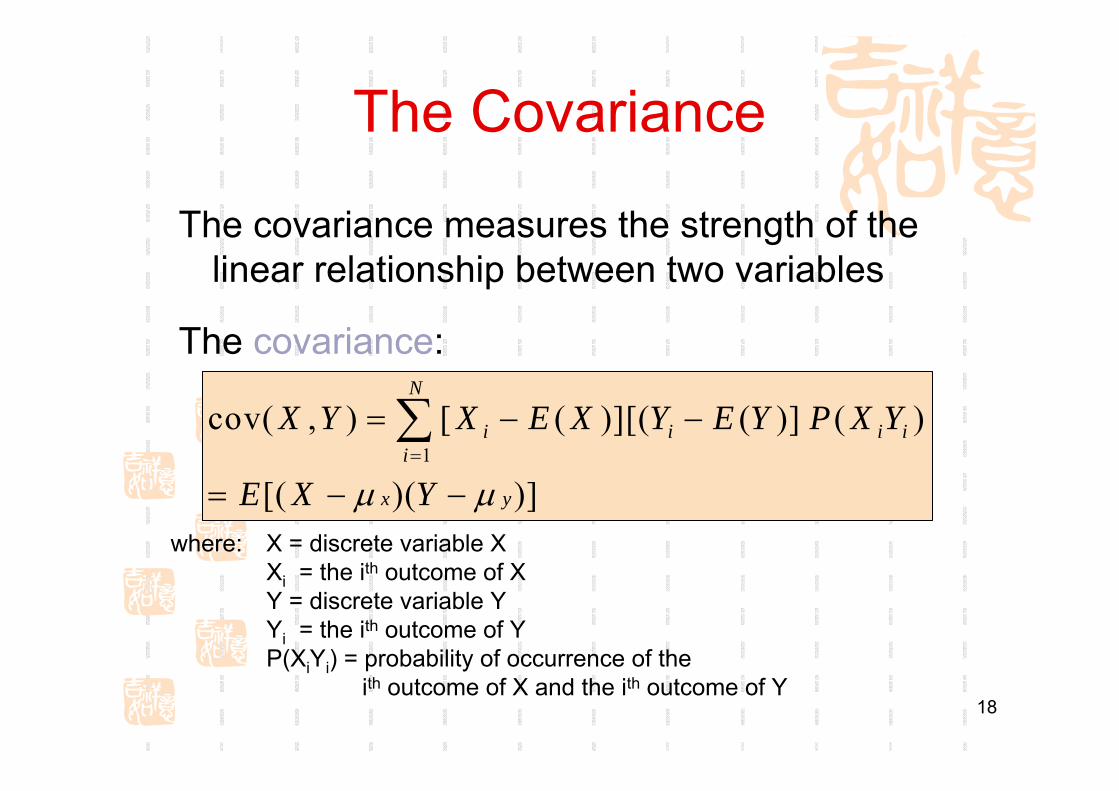
The Covariance

The covariance measures the strength of the linear relationship between two variables

The covariance:

1

cov( , ) [ ( )][( ( )] ( )

[( )( )]

N

i i i ii

x y

X Y X E X Y E Y P X Y

E X Yμ μ=

= − −

= − −

∑

where: X = discrete variable XXi = the ith outcome of XY = discrete variable YYi = the ith outcome of YP(XiYi) = probability of occurrence of the

ith outcome of X and the ith outcome of Y

19

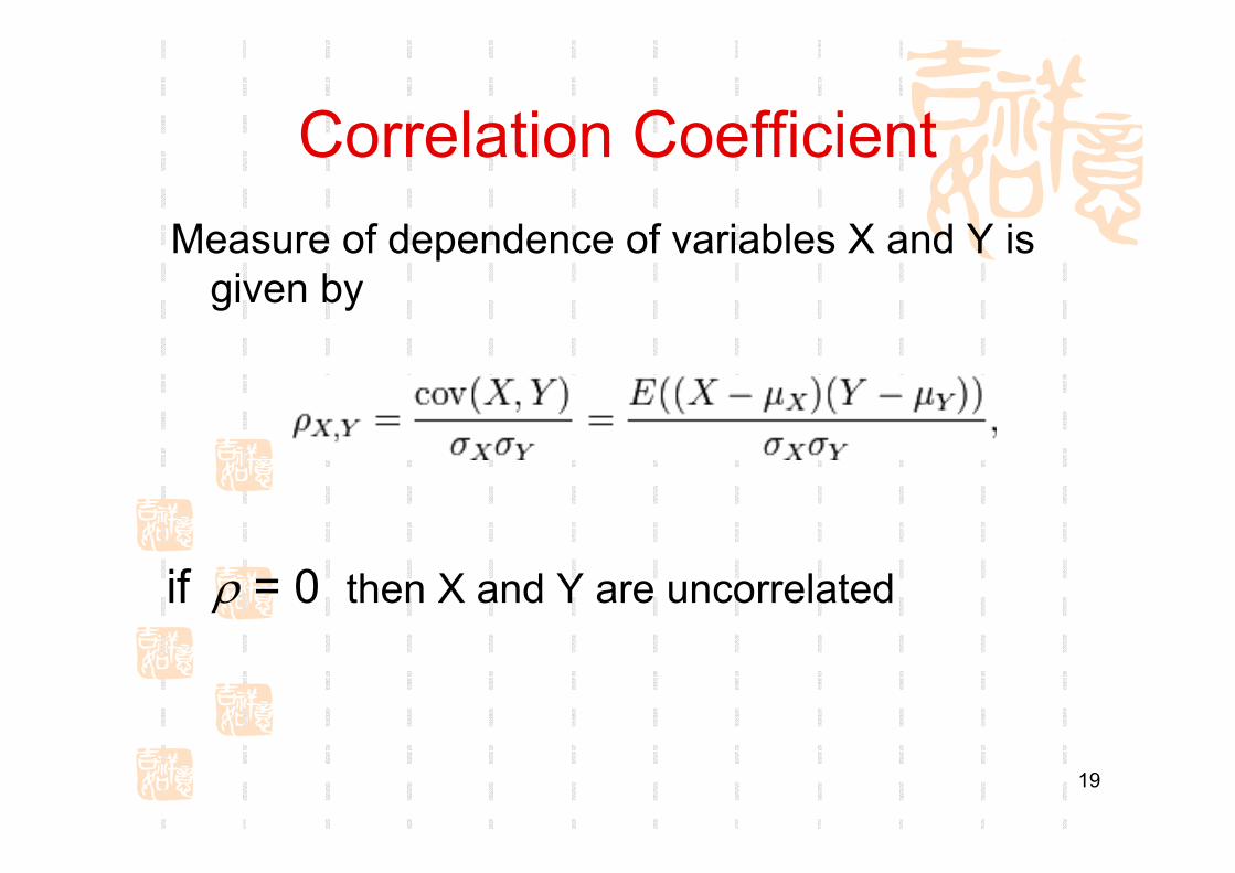
Correlation Coefficient

if ρ = 0 then X and Y are uncorrelated

Measure of dependence of variables X and Y is given by

20

Probability Distributions

ContinuousProbability

Distributions

Binomial

Poisson

Probability Distributions

DiscreteProbability

Distributions

Normal

Uniform

ExponentialMultinomial

21

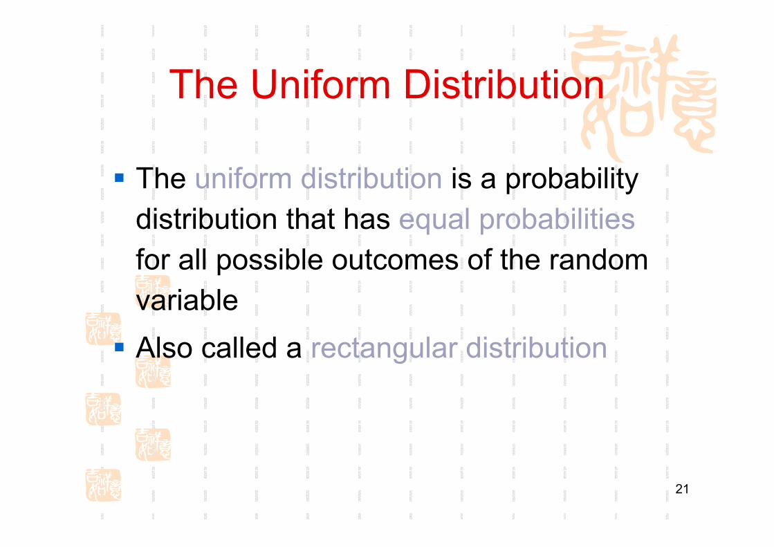
The Uniform Distribution

The uniform distribution is a probability distribution that has equal probabilitiesfor all possible outcomes of the random variableAlso called a rectangular distribution

22

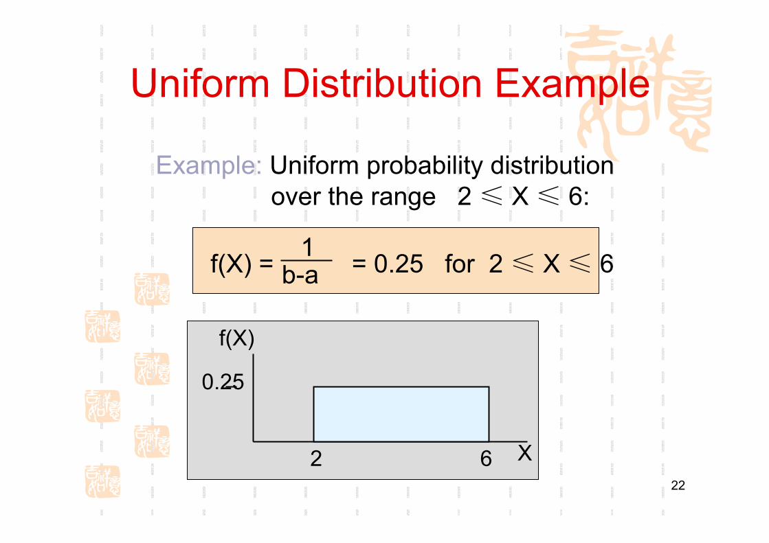
Uniform Distribution Example

Example: Uniform probability distributionover the range 2 ≤ X ≤ 6:

2 6

0.25

f(X) = = 0.25 for 2 ≤ X ≤ 6b-a1

X

f(X)

23

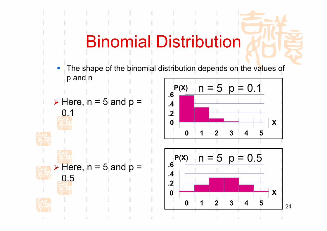
P(X=c) = probability of c successes in n trials,Random variable X denotes the number of ‘successes’ in n trials, (X = 0, 1, 2, ..., n)

n = sample size (number of trials or observations)

p = probability of “success” in a single trial(does not change from one trial to the next)

P(X=c)n

c ! n cp (1-p)c n c!

( )!=

−−

Binomial Distribution Formula

24

n = 5 p = 0.1

n = 5 p = 0.5

Mean

0.2.4.6

0 1 2 3 4 5X

P(X)

.2

.4

.6

0 1 2 3 4 5X

P(X)

0

Binomial DistributionThe shape of the binomial distribution depends on the values of p and n

Here, n = 5 and p = 0.1

Here, n = 5 and p = 0.5

25

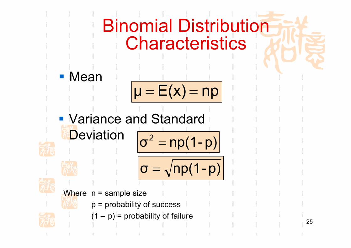
Binomial Distribution Characteristics

Mean

Variance and Standard Deviation

npE(x)μ ==

p)-np(1σ2 =

p)-np(1σ =

Where n = sample sizep = probability of success(1 – p) = probability of failure

26

Multinomial Distribution

P(Xi=Ci….Xk=Ck) = probability of having xi outputs in n trials,

Random variable Xi denotes the number of Observations of event i in ntrialsn = sample size (number of trials

or observations)pi= probability of event i

Example: You have 5 red, 4 blue and 3 yellow balls

(p =[ 0.42, 0.33, 0.25])

Question: probability that we get 2 red, 3 bule and 1

yellow;

11

1 2

( ) ...., ,...,

kCCk

k

np p p

C C C⎛ ⎞

= ⎜ ⎟⎝ ⎠

C

27

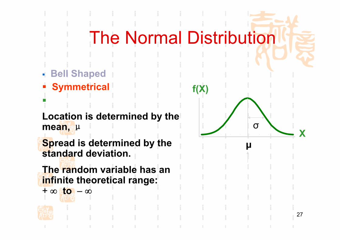
The Normal Distribution

‘Bell Shaped’Symmetrical

Location is determined by the mean, μSpread is determined by the standard deviation. The random variable has an infinite theoretical range: + ∞ to − ∞

X

f(X)

μ

σ

28

The formula for the normal probability density function is

Where e = the mathematical constant approximated by 2.71828π = the mathematical constant approximated by 3.14159μ = the population meanσ = the population standard deviationX = any value of the continuous variable

2μ)/σ](1/2)[(Xe2π1f(X) −−=

σ

29

Finding Normal Probabilities

Suppose X is normal with mean 8.0 and standard deviation 5.0Find P(X < 8.6) = 0.5 + P(8 < X < 8.6)

X

8.68.0

30

Thanks!