Prices versus Preferences:

Taste Change and Revealed Preference

Abi Adams (Oxford and IFS), Richard Blundell (UCL and IFS),

Martin Browning (Oxford and IFS), and Ian Crawford (Oxford and IFS)

December 2013, this draft January 2016∗

Abstract

A systematic approach for incorporating taste variation into a revealed preference framework for hetero-

geneous consumers is developed. This enables the recovery of the minimal variation in tastes required to

rationalise observed choices. It is used to examine the extent to which changes in tobacco consumption

are driven by price changes or by taste changes, and whether the significance of these two channels varies

across socioeconomic groups. A censored quantile approach accounts for unobserved heterogeneity. Sta-

tistically significant educational differences in the marginal willingness to pay for tobacco are recovered

with more highly educated cohorts experiencing a greater shift in their tastes.

∗We would like to thank Laurens Cherchye, Dennis Kristensen, Arthur Lewbel and participants at the CAM workshop,cemmap workshop and the AEA meetings session on consumer demand for helpful comments. The authors also gratefullyacknowledge financial support from the Economic and Social Research Council Centre for the Microeconomic Analysis ofPublic Policy at IFS and the European Research Council grant MicroConLab. All errors are ours.

1

1 Introduction

Structural empirical research on consumer behaviour is typically based upon the idea of choice-revealed

preference: consumers choose what they prefer from the options available to them and thereby reveal their

preferences through repeated observations of their choices from different budget sets. Simple techniques

can then be used to recover a consumer’s preferences from data on their choices using methods developed

by Samuelson (1948), Houthakker (1953), Afriat (1967) and Varian (1982). However, classical revealed

preference methods can only be applied when preferences are stable. If preferences change during the period

of observation then these methods cannot solve the inverse problem.

In this paper we develop a systematic approach to examine taste change within a revealed preference

(RP) framework. We create a methodology that recovers the minimal variation in tastes that is required to

rationalise observed choices. The patterns revealed by this exercise may suggest fruitful extensions to the

deterministic taste model. Patterns of taste changes that appear to vary systematically over time may be

diagnostic of, for example, unmeasured quality change, the spread of unobserved complimentary technologies,

or information acquisition. Patterns of taste change that vary systematically over consumer characteristics

may be evidence of preference heterogeneity. Patterns of taste variation which appear simply random may

be diagnostic of mistakes or measurement errors.

We represent taste heterogeneity as a linear perturbation to a base utility function, much as in McFadden

and Fosgerau (2012) and Brown and Matzkin (1998). Under this specification, taste change can be interpreted

as the shift in the marginal utility of a good for each individual. We show that this specification is not at

all restrictive. We derive inequalities that are an extension of Afriat (1967) such that when they hold there

exists a well-behaved base utility function and a series of taste shifters that perfectly rationalise observed

behaviour. We then show, under mild assumptions on the characteristics of available choice data, that we

can always find a pattern of taste shifters on a single good that are sufficient to rationalise any finite time

series of prices and quantities.

We apply this approach to pseudo-panel data to analyse the preferences for a good where there is strong

prima facie evidence that tastes have changed: tobacco products. In particular, we ask how much of the fall

in tobacco consumption is due to a rise in the relative price of tobacco and how much needs to be attributed

1

to taste changes? We also consider how tastes evolve across different socio-economic strata, asking the

question: Does education matter? The approach is implemented on household consumer expenditure survey

data using RP inequality conditions on the censored conditional quantile demand functions for tobacco. We

extend the analysis to allow for the non-separability of tobacco consumption from alcohol consumption.

Our objective is both better to understand the pattern of taste changes and to inform policy on the

balance between information/health campaigns and tax reform. Governments have a limited set of levers

should they wish to influence household consumption patterns. These include quantity constraints, price

changes through taxes and subsidies and information programs. The relative efficacy of the different modes

is important for designing public policy. The approach in this paper allows us to consider the extent to

which changes in tobacco consumption are due to price changes and how much is due to preference change.

This paper proceeds as follows. Sections 2 and 3 outline our theoretical framework and derive the neces-

sary and sufficient conditions under which observed behaviour and our model of taste change are consistent.

Section 4 develops a quadratic programming methodology that can be applied to recover the minimal amount

of interpersonally comparable taste variation that is necessary to rationalise choice behaviour. Section 5 in-

troduces the data used for our empirical investigation of tobacco consumption in the UK and discusses the

construction of quantity sequences for the psuedo-panel data that we construct from the UK Family Expen-

diture Survey using censored quantile regression methods. Section 6 applies our method to rationalise the

changes in tobacco consumption occurring in the U.K. since 1980. Finally, Section 7 concludes our analysis

and considers the implications of our findings for government anti-smoking policy moving forward.

2 Theoretical framework

Consider a consumer who selects a quantity vector q ∈ RK+ at time t to maximise their time-dependent

utility function:

u(q; αt) = v(q) + α′tq (1)

subject to p′q = x, where p ∈ RK++ is an exogenous price vector and x is total expenditure. It is assumed

that u(q, αt) is locally nonsatiated and concave conditional on αt ∈ RK , where αt is a vector of marginal

2

utility perturbations that indexes the consumer’s tastes at time t. This utility function therefore consists

of two components: a set of “base” preferences given by v(q), and a time-varying part given by α′tq.1 Our

use of marginal utility shifters to capture taste changes follows the random utility approach of Brown and

Matzkin (1998) and McFadden and Fosgerau (2012).

In this most general case, in which the marginal utility of all goods is potentially subject to arbitrary

observation-to-observation changes, choice patterns are not restricted by the model. To see this, take a

dataset D that is made up of a sequence of price-quantity observations for a consumer D = {pt,qt}t=1,...,T .

We can always find a sequence of taste-shifters {αt}t=1,...,T that can rationalise the model. To see this,

consider the first order conditions

∇u(qt) = ∇v(qt) + αt ≤ λtpt

This can be rewritten in terms of the base preferences and shadow prices as

∇v(qt) ≤ λtpt

where we use the shadow prices

pt = pt −αt

λt

where αt/λt represents the innovations in willingness-to-pay or ‘taste-wedge’ for every good in every period.

The behaviour generated by the model

maxq

v(q) + α′tq subject to p′

tq = xt

is therefore identical to the behaviour generated by the model

maxq

v(q) subject to p′tq = xt

where preferences are not subject to taste change, but where the prices and budget are replaced by their

1The effect of the taste change parameters αt on consumer demand is not invariant to transformations of v(q) and so furtheranalysis is conditioned upon a given cardinal representation of the ”base” preferences.

3

virtual counterparts.2 Thus the question of whether there exist rationalising taste-shifters is equivalent to

the question of whether we can always find shadow prices which can rationalise the observed quantity data.

Varian (1988, Theorem 1) shows that this is the case; indeed, there will typically be multiple suitable shadow

values consistent with any finite dataset.

This model of taste change, which allows for adjustments in the willingness-to-pay for every good in every

period, introduces as many free parameters as there are observations and so is clearly extremely permissive

- even given its apparently restrictive additive form. Instead, suppose that we have prior grounds to believe

that the most significant taste changes which have taken place have been confined to a single good, denoted

good 1. For example, in our empirical application, we suppose that good 1 represents tobacco products - a

good for which there are strong grounds for believing that tastes have changed significantly given increased

awareness of ill health effects. With the restriction of taste change to a single good, then αt = [α1t , 0, ..., 0]′,

yielding the following temporal series of utility functions:3

u(q; α1t ) = v(q) + α1

t q1 (2)

Taste changes thus enter the basic utility maximisation framework in a more restricted manner. Specifically,

the additive-linear specification for taste perturbations implies that the marginal rate of substitution between

any of the other goods j, k ∈ {2, ...,K} is invariant to taste instability on good-1. Another implication of

this functional form is that preferences will obey the single crossing property.

Definition (Milgrom and Shannon, 1994) A utility function u(q; α1t ) satisfies the single crossing property

in (q; α1) if for q′ > q′′ and α1′ > α1′′

u(q′; α1′′) ≥ u(q′′; α1′′) ⇒ u(q′; α1′) ≥ u(q′′; α1′) (3)

This condition can be interpreted as stating that for any q′ > q′′, the function f(α1) = u(q′; α1)−u(q′′; α1)

2The concept of a virtual budget was first suggested by Rothbarth (1941) and Neary and Roberts (1980) to develop thetheory of choice behaviour under rationing.

3This assumes intertemporal separability. Whether this is appropriate for the study of tobacco depends on the definition ofthe time period and the frequency of consumption observations. In our empirical application, this frequency is two years —there is evidence that this is sufficient time for habits to weaken (see, for example, Cuzbek and Johal (2010)).

4

crosses the horizontal axis only once, from negative to positive, as α1 increases. The single-crossing property

means that there is an unambiguous ranking of tastes over time for the good of interest. For example,

αt > αs implies that a consumer’s taste for good-1 is higher at t than at s. That is, the marginal rate of

substitution with respect to good-1 is always higher at t than at s at every point in commodity space.4

2.1 Empirical conditions

We are interested in establishing whether a consumer’s observed choice behaviour, D = {pt,qt}t=1,...,T , could

have been generated by taste change on a single good. Rationalisation of D by our model is defined as follows.

Definition 2 A consumer’s choice behaviour, D = {pt,qt}t=1,...,T , can be ‘good-1 taste rationalised’ by the

base utility function v(q) and a temporal series of additive linear perturbations to the marginal utility of

good-1, {α1t}t=1,...,T , if

v(q) + α1t q

1 ≤ v(qt) + α1t q

1t (4)

for all q such that:

p′tq ≤ p′

tqt (5)

In words, D can be rationalised by the model if there exists a time-invariant base utility function, v(q) and

a series of perturbations to the marginal utility of good-1 such that observed choices are weakly preferred

to all feasible alternatives. The empirical conditions, involving only observables, that are equivalent to a

rationalisation of D by our theoretical model are given in Theorem 1.

Theorem 1. The following statements are equivalent:

1. Observed choice behaviour, D = {pt,qit}t=1,...,T , can be good-1 taste rationalised.

2. One can find sets {vt}t=1,...,T , {α1t}t=1,...,T and {λt}t=1,...,T with λt > 0 for all t = 1, ..., T , such that

4In the empirical section of this paper, we will motivate the use of quantile regression methods by appeal to the fact thatan extension of our model, which directly includes interpersonal time-invariant heterogeneity, satisfies single crossing. In thetwo-good case, a basic result of single crossing is that arg maxq1 u(q1, q0; α1) increases with α1 (see Milgrom and Shannon(1994)).

5

there exists a non-empty solution set to the following revealed preference inequalities:

vs − vt + α1t (q

1s − q1

t ) ≤ λtp′t(qs − qt)

α1t ≤ λtp

1t

(6)

Theorem 1 is implied by optimising behaviour within the theoretical framework. If there exists a non-

empty solution set to the inequalities defined by Theorem 1, then there exists a well-behaved base utility

function and a series of taste shifters on good-1 that perfectly rationalise observed behaviour. The variables

referred to by the revealed preference inequalities in part (2) of Theorem 1 have natural interpretations.

The numbers {ut}t=1,..,T and {λt}t=1,..,T can be interpreted respectively as measures of the level of baseline

utility and the marginal utility of income at observed demands. The α1t values can be interpreted as the

marginal utility perturbation to good-1 relative to that dictated by base utility at observed demands since

we can set α1t = 0 for all t.

Theorem 1 is an extension to the equivalence result originally derived by Afriat (1967) for the utility

maximisation model with a time-invariant utility function. Imposing α1t = 0 for all t = 1, .., T returns the

standard Afriat inequalities. If there is no intertemporal variation in good-1, q1t = q1

s for all t, s ∈ 1, ..., T ,

then we immediately have the standard Afriat conditions.5

Given solutions for condition (2) in Theorem 1, we can construct a rationalising utility function at each

observation (u(qt; α1t )) and also examine counterfactuals such as at u(qt; α1

s). This indicates the utility

which would be derived from consuming the period t bundle, but with one’s tastes from another period. For

example, comparing u(qt; α1t ) with u(qt; α1

s) gives

u(qt; α1t ) − u(qt; α

1s) =

(α1

t − α1s

)q1t

whilst the shadow price of consumption of good 1 in period t given period s tastes is

u1(qt; α1s) = λt

[

p1t −

(α1

t − α1s

)

λt

]

5In what follows we assume that we assume that we observe period-to-period variation in good-1 such that q1t 6= q1

s for allt, s = 1, ..., T .

6

Note that the shadow price of consumption in period t, given tastes in period s, may be negative if the taste-

change term(α1

t − α1s

)is large enough. For example, if the consumer’s taste for tobacco changes negatively

between some earlier period t − 1 and a later period t such that α1t−1 − α1

t is sufficiently positive then it is

possible that

u1(qt−1; α1t ) = λt−1

[

p1t−1 −

(α1

t−1 − α1t

)

λt−1

]

< 0

The interpretation of this is that the consumer in period t would need to be paid to smoke as much as they

did back in period t − 1.

Solutions to Theorem 1 also enable us to construct the virtual prices at which the individual with

preferences given by the base utility function would have purchased the bundle of goods purchased at t with

taste for tobacco α1t

p1t = p1

t −α1

t

λt

Interpreting taste change as an evolution of virtual prices supports the interpretation of information pro-

grammes as supplementary tax and incomes policies. For example, programmes designed to cultivate a

negative taste for tobacco can be thought as levying a ‘taste-tax’ on the good because they manifest them-

selves in a rise in the virtual price for tobacco: p1t > p1

t as α1t < 0 for a negative taste perturbation. Given

the virtual price characterisation, variation in α1 is more easily interpreted as a change in the marginal

willingness to pay for good-1. The magnitude of the change in the marginal willingness to pay is captured

by the term α1t /λt. This is useful because there is no clear behavioural interpretation of the magnitude of

α1t since its value depends upon the cardinal representation of base preferences.

2.2 Rationalisability

Surprisingly, under mild assumptions on D,6 observed behaviour can always be explained by our simple

model; that is, one can find sets of base-utility numbers, {vt}t=1,...T , marginal utilities of income {λt}t=1,...,T

and taste perturbations on a single good {α1t}t=1,...,T that rationalise observed choice behaviour.

6Our assumption that we observe period-to-period variations in quantities such that qkt 6= qk

s for all t, s = 1, ..., T is importanthere.

7

Theorem 2 Given q1t 6= q1

s for all t and s, any data set D can be good-1 taste rationalised.

Note that quantity variation is sufficient, but not necessary, for D to be good-1 taste rationalised. Let

p¬1t denote the price vector for all goods except good-1, p¬1

t = [p2t , ..., p

Kt ], and define q¬1

t analogously. For

subsets St ⊆ {1, ..., T } within which q1t = q1 for all t ∈ St, if the choice set {p¬1

t ,q¬1it }t∈St

satisfies the

Generalised Axiom of Revealed Preference (GARP), then D will be rationalisable by our framework despite

the violation of perfect variation in good-1. A leading example of this is when an agent does not buy good

1 in more than one period (q1s = q1

t = 0 for some s 6= t).

Theorem 2 is closely related to Varian’s (1988) Theorem 1, in which it is proved that the standard

utility maximisation model is virtually emptied of empirical content if the price of at least one good is not

observed. In such circumstances, one can hypothesize that the unobserved prices take on values high enough

that expenditures on goods with unobserved prices dominate all other revealed preference comparisons. The

virtual budget characterisation of taste change makes clear the connection between Theorem 2 and Varian’s

result: tastes for good-1 could always decline to the extent that the virtual prices required to support

observed bundles are high enough to prevent an intersection of the virtual budget hyperplanes.

2.3 Recoverability

The revealed preference inequalities associated with our theoretical framework can be used to recover the

set of minimal perturbations to the marginal utility of good-1 that will rationalise observed behaviour. This

set is always non-empty if D satisfies perfect variation with respect to good-1. We here outline an easy

to implement quadratic programming procedure that enables the recovery of the minimal marginal utility

perturbations on good-1 that are necessary to rationalise a data set D.

Recovery of α1 The minimal squared perturbations to the marginal utility of good-1 relative to preferences

in period 1 that are necessary to good-1 rationalise observed choice behaviour D = {pt,qt}t=1,...,T are

8

identified as the unique solution set {α1t}t=1,...,T to the following quadratic programme.

min{vt,λt,αt}t=1,...,T

T∑

t=1

(α1

t

)2(7)

subject to:

1. The revealed preference inequalities:

vs − vt + α1t (q

1s − q1

t ) ≤ λtp′t(qs − qt)

α1t ≤ λtp

1t

(8)

2. The normalisation conditions:

v1 = δ (an arbitrary constant)

λ1 = β (a strictly positive constant)

α11 = 0

(9)

for s, t = 1, ..., T .

Minimising the sum of squared α1’s subject to the set of revealed preference inequalities ensures that

the recovered pattern of minimal taste perturbations are sufficient to rationalise observed choice behaviour.

The normalisation conditions are required because the quadratic programming problem is ill-posed in their

absence. This is due to the invariance of tastes to positive monotonic changes in the utility function. Let

{vt, λt, α1t}t=1,...,T represent some feasible solution to the rationalisation constraints. As the set represents

a feasible solution, the following inequalities hold for all s, t ∈ {1, ..., T }:

vs − vt + αt(q1s − q1

t ) ≥ λsp′s(qs − qt) (10)

However, the following set of inequalities is also feasible:

β(vs + δ) − β(vt + δ) + βα1t (q

1s − q1

t ) ≥ βλsp′s(qs − qt) (11)

9

for δ ∈ (−∞,∞) and β > 0. Thus, without a location and scale normalisation, there exist an infinite

number of feasible sets of utility numbers that can be associated with a given set of feasible taste shifters.

Without loss of generality, we impose α11 = 0, which allows us to interpret {α1

t}t=2,...,T as the minimal

rationalising marginal utility perturbations to good-1 relative to preferences at t = 1. We also impose the

scale normalisation λ1 = β to ensure that the output of the quadratic programming procedure is scaled

sensibly.

3 Rationalising tobacco consumption

In this section we apply our revealed preference methodology to study taste changes with respect to tobacco

in the UK. Over the period we examine (1980 to 2000), the UK population acquired more information about

the ill-effects of smoking, perhaps causing tastes for tobacco to change. The Health and Lifestyle Survey

1984 and the Office for National Statistics Omnibus Survey 1996, for example, both asked questions about

the connection between smoking and poor health. Between these years, there was a large rise in awareness

of the link between smoking and heart disease; in 1984, only 25.8% of the sample believed that smoking

caused heart disease, while by 1996, 80.6% recognised the link. Thus we argue that there is indeed strong

prima facie evidence that tastes have changed in a particular direction, and we would therefore expect that

our approach should be able to identify this.

3.1 The data

There is no UK consumption panel that includes spending on tobacco and covers a sufficiently long time

period. However we do have rich cross section consumption data in the Family Expenditure Survey (FES).

The FES records detailed expenditure and demographic information for 7,000 randomly selected households

each year and we use the FES with biennial periodicity between 1980 and 2000.7 From this dataset, we

construct two pseudo-panels according to education levels using the cohort of individuals who were aged

between 25 and 35 years old in 1980 (i.e. they were born between 1945 and 1955).8 The “low” education

7We restrict observations to biennial periodicity to reduce the salience of habit formation in tobacco for our method and tolimit the computational burden of the procedure.

8We select this birth cohort because less than 5% of smokers start smoking after they reach their 25 th birthday (Office forNational Statistics, 2012). The assumption that the population of smokers is stable is then relatively mild.

10

group, L, is formed from those individuals who left school no older than the legal minimum, 15 years old at

the time. Those staying in school past this age comprise a “high education” group, H. In each period, there

are between 737 and 1079 individuals forming the low education pseudo-cohort, and between 376 and 460

individuals forming the high education pseudo-cohort. Appendix B provides further details and summary

statistics.

We are primarily concerned with choice over a tobacco aggregate and a nondurable commodity aggregate,

i.e the number of goods is reduced to. K = 2. Appendix B provides a detailed list of goods that are classed

as nondurables in our data set. Total expenditure is defined as all spending on these goods. Price indices

are constructed for the tobacco and nondurable aggregates using the sub-indices of the U.K. Retail Price

Index.

3.2 Quantile demands

In experimental revealed preference analyses, recovery exercises are typically conducted on an individual-

by-individual basis in the laboratory. Indeed, this is the implicit setting assumed in our theoretical set-up.

However, our aim here is to apply the analysis developed above to a representative sample of consumers from

a long time-series of repeated cross-section data. Given the structure of our data, we pool information across

different individuals in a pseudo-panel and use quantile demands to recover individual demand behaviour.

We will then apply the revealed preference methodology to estimated quantities in order to make statements

about taste changes over time for the population of interest. This approach places restrictions on unobserved

time invariant interpersonal heterogeneity which we now address.

In each period t = 1, ..., T and for each pseudo-cohort c = {L,H}, let us observe individuals i = 1, ..., N ct .

For notational simplicity, the cohort and individual subscripts are suppressed for the rest of this section.

Drawing on Blundell, Kristensen and Matzkin (2014), we assume that individual demands are monotonic in

scalar unobserved heterogeneity and restrict the dimensionality of the demand system to K = 2. Good 1 is

tobacco, our good of interest. To allow for heterogeneity, we augment individual preferences in (2) to take

11

the form:

u(q; αt) = f(q1, q0, τ ) + α1t q

1 (12)

where τ ∼ U(0, 1) represents time-invariant interpersonal taste heterogeneity and α1t gives the perturbation

to the marginal utility of good 1 experienced by that individual consumer at time t, as in (2).

For quantile demands to identify individual demands we have to place further restrictions on preferences

that guarantee demands are monotonic in unobserved scalar heterogeneity. Matzkin (2007) provides the

following general conditions on heterogeneous preferences f(q1, q0, τ ) to be invertible in unobserved hetero-

geneity

f(q1, q0, τ ) = f(q1, q0) + w(q1, τ ) (13)

where the functions f and w are twice continuously differentiable, strictly increasing and strictly concave,

and w(q1, τ ) has a strictly positive second derivative. Under these conditions, the demand function for q1

will satisfy the restrictions of consumer choice for each value τ . Similarly, budget shares will be monotonic

in τ .

Preferences displaying taste change then have the form:

u(q; αt) = f(q1, q0) + w(q1, τ ) + α1t q

1

= f(q1, x − p1q1) + τ q1 + α1t q

1. (14)

With only interpersonal time-invariant heterogeneity (i.e. α1t = 0 for all t = 1, ..., T ), invertibility guarantees

the family of preferences {f(q1, x − p1q1) + τ q1} obeys single-crossing. Thus, in this context, quantile

demands, conditional on (p, x), identify individual demands (see Blundell et al (2014) for further discussion).

12

Let q1(p, x, τ ) give the demand for good 1 that is associated with taste heterogeneity τ . Then,

q1(p, x, τ ) = maxq1

f(q1, x − p1q1) + τq1

= Qq1(τ |p, x) (15)

where Qq1(τ |p, x) denotes the τ ′th conditional quantile of q1.

To equate quantile and individual demands given the time varying component to unobserved preference

heterogeneity, α1t , we further assume that taste evolution term (τ + α1

t )q1 does not alter the ranking of

consumers over time in the q1 distribution conditional on (p, x). While this is a strong assumption, we do

not believe it to be incredible; we only consider individuals who are old enough to have made an initial

decision to smoke (see above) and high profile anti-smoking campaigns are not targeted in a way that

would cause one to expect significant re-ranking within education cohorts. With these assumptions, the

τ ’th conditional quantile reflects the demand behaviour of an individual with unobserved time-invariant

preference heterogeneity τ and α1t q

1.

In the following sections, we will rationalise the changes in tobacco consumption at three different quan-

tiles of the budget share for tobacco distribution, τ ∈ {0.55, 0.65, 0.75}, for each psuedo-panel. We refer

to the 0.55-quantile as “light smokers”, to the 0.65-quantile as “moderate smokers” and we refer to the

0.75-quantile as “heavy smokers”. We thus recover taste changes for six different “individuals”. Figure 1

displays the (unconditional) budget shares for tobacco at the relevant quantiles of both education psuedo-

panels between 1980 and 2000. At each quantile, the high education cohort devotes a smaller proportion

of their budget to tobacco than the low education cohort. In fact, within the high education cohort, the

0.55 quantile of the budget share for tobacco distribution falls to zero in 1983 and remains nil for the the

rest of the period considered, while the 0.65 quantile is zero by the end of the period. Tobacco consumption

remains strictly positive in all periods for the quantiles of the low education cohort that are considered.

13

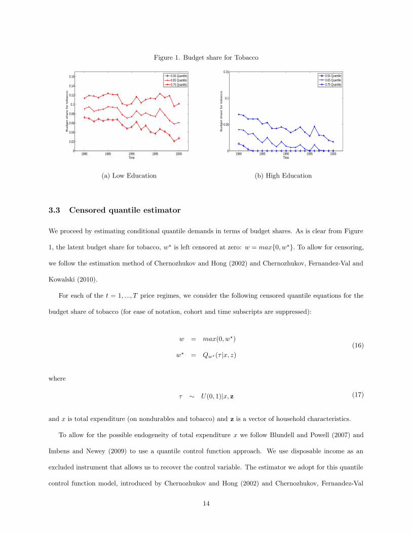
Figure 1. Budget share for Tobacco

1980 1985 1990 1995 20000

0.02

0.04

0.06

0.08

0.1

0.12

0.14

0.16

Time

Bu

dg

et

sh

are

fo

r to

ba

cco

0.55 Quantile0.65 Quantile0.75 Quantile

1980 1985 1990 1995 20000

0.05

0.1

0.15

Time

Bu

dg

et

sh

are

fo

r to

ba

cco

0.55 Quantile0.65 Quantile0.75 Quantile

(a) Low Education (b) High Education

3.3 Censored quantile estimator

We proceed by estimating conditional quantile demands in terms of budget shares. As is clear from Figure

1, the latent budget share for tobacco, w? is left censored at zero: w = max{0, w?}. To allow for censoring,

we follow the estimation method of Chernozhukov and Hong (2002) and Chernozhukov, Fernandez-Val and

Kowalski (2010).

For each of the t = 1, ..., T price regimes, we consider the following censored quantile equations for the

budget share of tobacco (for ease of notation, cohort and time subscripts are suppressed):

w = max(0, w?)

w? = Qw?(τ |x, z)

(16)

where

τ ∼ U(0, 1)|x, z (17)

and x is total expenditure (on nondurables and tobacco) and z is a vector of household characteristics.

To allow for the possible endogeneity of total expenditure x we follow Blundell and Powell (2007) and

Imbens and Newey (2009) to use a quantile control function approach. We use disposable income as an

excluded instrument that allows us to recover the control variable. The estimator we adopt for this quantile

control function model, introduced by Chernozhukov and Hong (2002) and Chernozhukov, Fernandez-Val

14

and Kowalski (2010), is given by

Qw?(τ |x, z, v) = X′β(τ) (18)

where v is the unobserved latent control variable that is included to account for the possible endogeneity

of x. In implementation, X is replaced with X = [log(x), log(x)2, z, v], where v is the conditional quan-

tile regression estimate of v and where the the OECD demographic index is used to capture demographic

characteristics, z.

For each education group at each price regime, β(τ) is estimated as:

β(τ) = arg minβ

∑

i∈S

ρτ (wi − X′iβ) (19)

where ρτ is the standard asymmetric absolute loss function of Koenker and Bassett (1978) and S denotes the

set of observations for which Pr(wi > 0) > δ, i.e. those for which the probability of censoring is negligible

and a linear functional form for the conditional quantile is justified. We refer the reader to Chernozhukov,

Fernandez-Val and Kowalski (2010) for a more detailed exposition, including the construction of S.

Reviving the cohort and time subscripts, the set of estimated quantities, at which taste changes are

recovered, are constructed as:

wct (τ) = Xc′

t βc

t(τ) (20)

qc,τt = xt

[wc

t

p1t

,(1 − wc

t )p0

t

]′(21)

for c = {L,H} and t = 1, ...., T and where Xct = [log(xc

t), log(xct)

2, 1, 0]. xct are expenditure levels set to

ensure that the average demand in period t = 1, ..., T −1 is weakly affordable at the time t budget.9 By using

these expenditure levels, rather than, for example, mean cohort expenditure in a given period, we ensure

that budget lines at different time periods intersect. This is a necessary condition for detecting violations of

a time-invariant utility function in the data. For more details see Blundell, Browning and Crawford (2003,

2008).

9In the first period, expenditure is set equal to the cohort median.

15

3.4 Implementation

The quadratic programming procedure of Section 2 is applied to the set {pt,qc,τt }t=1,...,T , with c = {L,H}

and τ = {0.55, 0.65, 0.75} and qc,τt estimated as above. Application to the pooled choice set imposes a

common base utility function for all cohorts and quantiles . This is necessary because differences in the

base utility function across cohorts and quantiles could lead to a violation of single-crossing, precluding

one from making global statements about differences in the taste for tobacco across different cohorts and

quantiles (see Section 2). Taste changes are normalised relative to the heavy smoking, low education group

in 1980, αL,0.551980 = 0. Implementation of the method is a computationally intensive procedure. To limit the

computational burden of the empirical exercise, observations are restricted to biennial periodicity.

The procedure is bootstrapped to address the issue of sampling variation in estimated quantity sequences.

Observations are randomly drawn with replacement within each education-time cell 1000 times and quan-

tile demands are estimated on each resampled set of observations. Minimal taste change is estimated for

these sets of perturbed quantities, allowing us to construct a simultaneous 95% confidence interval on taste

perturbations for each cohort.

4 Results

We find significant differences in the virtual price trajectories along the SMP total expenditure path across

cohorts. Figures 2 and 3 depict the minimum virtual prices and the minimal taste wedge that are necessary

to rationalise the choice behaviour of the low and high education cohorts, given the normalisation of taste

shifters relative to the heavy-smoking low-education cohort in 1980. In addition to recovered virtual prices,

the observed relative price for tobacco is depicted. This is the trajectory that each cohort’s virtual price

would follow in the absence of intercohort and intertemporal taste heterogeneity. This represents the change

in the marginal willingness to pay for tobacco relative to base tastes along the SMP expenditure paths.

16

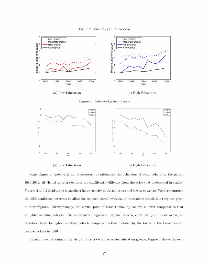
Figure 2. Virtual price for tobacco

1980 1985 1990 1995 20000

1

2

3

4

5

6

Time

Rel

ativ

e pr

ice

of to

bacc

o

Low smokerModerate smokerHigh smokerActual price

1980 1985 1990 1995 20000

1

2

3

4

5

6

Time

Rel

ativ

e pr

ice

of to

bacc

o

Low smokerModerate smokerHigh smokerActual price

(a) Low Education (b) High Education

Figure 3. Taste wedge for tobacco

1980 1985 1990 1995 2000-12

-10

-8

-6

-4

-2

0

2

Time

Ta

ste

we

dg

e: a

lph

a/la

mb

da

LowModerateHigh

1980 1985 1990 1995 2000-12

-10

-8

-6

-4

-2

0

2

Time

Ta

ste

we

dg

e: a

lph

a/la

mb

da

LowModerateHigh

(a) Low Education (b) High Education

Some degree of taste variation is necessary to rationalise the behaviour of every cohort for the period

1980-2000; all virtual price trajectories are significantly different from the price that is observed in reality.

Figures 2 and 3 display the intracohort heterogeneity in virtual prices and the taste wedge. We here suppress

the 95% confidence intervals to allow for an uncluttered overview of intracohort trends but they are given

in later Figures. Unsurprisingly, the virtual price of heavier smoking cohorts is lower compared to that

of lighter smoking cohorts. The marginal willingness to pay for tobacco, captured by the taste wedge, is,

therefore, lower for lighter smoking cohorts compared to that dictated by the tastes of the low-education

heavy-smokers in 1980.

Turning now to compare the virtual price trajectories across education groups, Figure 4 shows the evo-

17

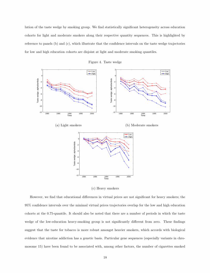
lution of the taste wedge by smoking group. We find statistically significant heterogeneity across education

cohorts for light and moderate smokers along their respective quantity sequences. This is highlighted by

reference to panels (b) and (c), which illustrate that the confidence intervals on the taste wedge trajectories

for low and high education cohorts are disjoint at light and moderate smoking quantiles.

Figure 4. Taste wedge

1980 1985 1990 1995 2000-12

-10

-8

-6

-4

-2

0

2

Time

Tas

te w

edge

: alp

ha/la

mbd

a

LowHigh

1980 1985 1990 1995 2000-12

-10

-8

-6

-4

-2

0

2

Time

Tas

te w

edge

: alp

ha/la

mbd

a

LowHigh

(a) Light smokers (b) Moderate smokers

1980 1985 1990 1995 2000-12

-10

-8

-6

-4

-2

0

2

Time

Tas

te w

edge

: alp

ha/la

mbd

a

LowHigh

(c) Heavy smokers

However, we find that educational differences in virtual prices are not significant for heavy smokers; the

95% confidence intervals over the minimal virtual prices trajectories overlap for the low and high education

cohorts at the 0.75-quantile. It should also be noted that there are a number of periods in which the taste

wedge of the low-education heavy-smoking group is not significantly different from zero. These findings

suggest that the taste for tobacco is more robust amongst heavier smokers, which accords with biological

evidence that nicotine addiction has a genetic basis. Particular gene sequences (especially variants in chro-

mosome 15) have been found to be associated with, among other factors, the number of cigarettes smoked

18

per day and nicotine intake (see, for example, Mansfelder (2000), Berrettini (2008), Keskitalo (2009)). Given

that one’s genome does not change except by random mutation, one would expect tastes grounded in genetic

factors to be relatively time invariant as they appear to be in the case of our heavy-smokers.

5 Conditional taste change

The estimation strategy we used above implicitly assumes that tobacco is weakly separable from all other

non-durables, including alcohol. To examine the robustness of our findings to this assumption, and to explore

whether additional patterns emerge from the data once this condition is relaxed, we follow the approach of

Browning and Meghir (1998) and re-run our quadratic programming procedure on quantile demands that are

estimated conditional on alcohol consumption. Specifically, we partition the set of observations that comprise

each education group into ”light” and ”heavy” drinkers depending on whether an individual consumes below

or above the median budget share for alcohol in that time period. The quantile regression method outlined

in the previous section is then applied to estimate demands within each education-alcohol-time cell at the

expenditures along the same SMP paths that were calculated previously. Base preferences are normalised

relative to those of the heavy smoking, heavy drinking, low education cohort in 1980.

Taste shifters are only estimated for moderate and heavy smokers that are drawn from our education-

alcohol cohorts. The requirement of perfect intertemporal variability of good-1 is violated for demands on the

“high education”-“light smoking”-“light drinking” cohort; for most of the period considered the estimated

budget share on tobacco for this cohort is zero. We thus do not calculate taste changes for light smokers.

This ensures that there will always exist a set of comparable, choice-rationalising taste shifters that can

be estimated in a reasonable amount of time. However, please note that the fact that light smokers are

not included at this stage implies that the magnitude of estimated taste shifters are not comparable to the

unconditional quantile results of the previous section.

We recognise that the rank invariance assumption, which is imposed by the quantile regression model

that is used to estimate SMP demands, is stronger in this context of conditional demands. It amounts to

a no re-ranking requirement on the joint distribution of tobacco-alcohol group budget shares. We cannot

determine how strong this assumption is because we do not have access to panel data for the period. However,

19

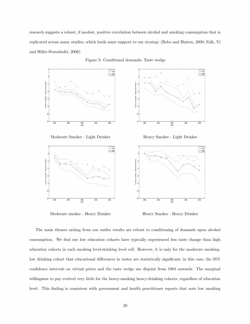
research suggests a robust, if modest, positive correlation between alcohol and smoking consumption that is

replicated across many studies, which lends some support to our strategy (Bobo and Husten, 2000; Falk, Yi

and Hiller-Sturmhofel, 2006).

Figure 5: Conditional demands- Taste wedge

1980 1985 1990 1995 2000-12

-10

-8

-6

-4

-2

0

2

Time

Ta

ste

we

dg

e: a

lph

a/la

mb

da

LowHigh

1980 1985 1990 1995 2000-12

-10

-8

-6

-4

-2

0

2

Time

Ta

ste

we

dg

e: a

lph

a/la

mb

da

LowHigh

Moderate Smoker - Light Drinker Heavy Smoker - Light Drinker

1980 1985 1990 1995 2000-12

-10

-8

-6

-4

-2

0

2

Time

Ta

ste

we

dg

e: a

lph

a/la

mb

da

LowHigh

1980 1985 1990 1995 2000-12

-10

-8

-6

-4

-2

0

2

Time

Ta

ste

we

dg

e: a

lph

a/la

mb

da

LowHigh

Moderate smoker - Heavy Drinker Heavy Smoker - Heavy Drinker

The main themes arising from our earlier results are robust to conditioning of demands upon alcohol

consumption. We find our low education cohorts have typically experienced less taste change than high

education cohorts in each smoking level-drinking level cell. However, it is only for the moderate smoking-

low drinking cohort that educational differences in tastes are statistically significant; in this case, the 95%

confidence intervals on virtual prices and the taste wedge are disjoint from 1984 onwards. The marginal

willingness to pay evolved very little for the heavy-smoking heavy-drinking cohorts, regardless of education

level. This finding is consistent with government and health practitioner reports that note low smoking

20

cessation rates amongst heavy drinkers (Dollar et al., 2009). It also motivates the use of further restrictions

on the joint consumption of alcohol and tobacco (e.g. bans on smoking in pubs and bars). Such restrictions

would exploit the complementarity between alcohol and tobacco to reduce smoking amongst the heavy-

smoking heavy-drinking group given the persistence in their tastes for tobacco.10

6 Conclusions

This paper has provided a theoretical and empirical framework for characterising taste change. We have

uncovered a surprising non-identification result: observational data sets on a K-dimensional demand system

can always be rationalised by taste change on a single good in a nonparametric setting. Our theoretical

results were used to develop a quadratic programming procedure to recover the minimal intertemporal (and

interpersonal) taste heterogeneity required to rationalise observed choices. The approach we have developed

establishes that we can almost always rationalise a data set when allowing for taste change in a single good.

We have shown that these conditions are equivalent to solving a “latent virtual price” problem.

A censored quantile approach was used to allow for unobserved heterogeneity and censoring in the ap-

plication of our approach to the consumption of tobacco in the UK over the period 1980 to 2000 where we

might expect large shifts in demand due to taste change. Non-separability between tobacco and alcohol

consumption was incorporated using a conditional (quantile) demand analysis.

We focussed on a single birth cohort aged between 25 and 35 years old in 1980 and allowed for examined

different education groups. The estimation results suggested that systematic taste change was required for all

groups in our expenditure survey data. In no case could the fall in tobacco consumption over the twenty year

period be rationalised solely by the rise in the relative price of tobacco. A series of negative perturbations to

the marginal utility of tobacco were found to be sufficient to rationalise the trends in tobacco consumption.

Statistically significant educational differences in the marginal willingness to pay for tobacco were recov-

ered; more highly educated cohorts experienced a greater shift in their effective tastes away from tobacco.

We find virtual prices and the taste wedge are disjoint across education groups for all cohorts except for

the “heavy smoking”-“heavy drinking” group. Education is largely irrelevant for explaining the evolution of

10See Adda and Cornaglia (2010) for additional effects of such restrictions.

21

virtual prices amongst heavy smokers. This might suggest diminished differences in smoking behaviour by

education group in the future.

References

[1] Jerome Adda and Francesa Cornaglia (2010), “The Effect of Bans and Taxes on Passive Smoking”,American Economic Journal: Applied Economics, 2(1), 1-32.

[2] Sydney Afriat (1967), “The Construction of Utility Functions from Expenditure Data”, InternationalEconomic Review, 8(1), 67-77.

[3] Sydney Afriat (1977), The Price Index, London: Cambridge University Press.

[4] Laura Blow and Ian Crawford (1999), “Valuing Quality”, IFS Working Paper Series W99/21, TheInstitute for Fiscal Studies.

[5] Richard Blundell, Martin Browning, Laurens Cherchye, Ian Crawford, Bram De Rock and FredericVermeulen (2015), “Sharp for SARP: Nonparametric bounds on the behavioural and welfare effects ofprice changes”, American Economic Journal: Microeconomics, 7(1): 43–60

[6] Richard Blundell, Martin Browning and Ian Crawford (2003), “Nonparametric Engel Curves and Re-vealed Preference”, Econometrica, 71(1), 205-240.

[7] Richard Blundell, Martin Browning and Ian Crawford (2008), “Best Nonparametric Bounds on DemandResponses”, Econometrica, 76(6), 1227-1262.

[8] Richard Blundell, Dennis Kristensen and Rosa Matzkin (2014) “Bounding Quantile Demand Functionsusing Revealed Preference Inequalities”, Journal of Econometrics, 117, 112-127.

[9] Richard Blundell and James Powell (2007), “Censored Regression Quantiles with Endogenous Regres-sors”, Journal of Econometrics, 141(1), 65-83.

[10] Janet Bobo and Corinne Husten (2000), “Sociocultural Influences on Smoking and Drinking”, AlcoholResearch and Health, 24(4), 225-232.

[11] Donald Brown and Rosa Matzkin (1998), “Estimation of Nonparametric Functions in SimultaneousEquations Models, with an Application to Consumer Demand”, Cowles Foundation Discussion Papers1175, Cowles Foundation, Yale University.

[12] Martin Browning (1989), “A Nonparametric Test of the Life-Cycle Rational Expectations Hypothesis”,International Economic Review, 30(4) 979-992.

[13] Martin Browning and Costas Meghir (1991), “The Effects of Male and Female Labor Supply on Com-modity Demands”, Econometrica, 59(4), 925-951.

[14] Victor Chernozhukov and Han Hong (2002), “Three-Step Censored Quantile Regression and Extramar-ital Affairs”, Journal of the American Statistical Association, 40(459), 872-882.

[15] Victor Chernozhukov, Ivan Fernandez-Val and Amanda Kowalski (2010), “Quantile Regression withCensoring and Endogeneity”, Mimeo, Massachusetts Institute for Technology.

[16] Ian Crawford (2010), “Habits Revealed”, Review of Economic Studies, 77(4), 1382-1402.

22

[17] Department of Health (2011), White Paper: Healthy Lives, Healthy People: Our Strategy for PublicHealth in England, London: TSO.

[18] W. Erwin Diewert (1973), “Afriat and Revealed Preference Theory”, The Review of Economic Studies,40(3), 419-425.

[19] Charles Manski (2007), Identification for Prediction and Decision, Cambridge, MA: Harvard UniversityPress.

[20] Rosa L. Matzkin, (2007) “Heterogeneous Choice,” in Advances in Economics and Econometrics, Theoryand Applications, Ninth World Congress of the Econometric Society, edited by R. Blundell, W. Newey,and T. Persson, Cambridge University Press.

[21] Daniel McFadden and Mogens Fosgerau (2012), “A Theory of the Perturbed Consumer with GeneralBudgets”, NBER Working Papers 17953, National Bureau of Economic Research, Inc.

[22] Paul Milgrom and Chris Shannon (1994), “Monotone Comparative Statics”, Econometrica, 62(1), 157-180.

[23] Christopher Murray and Alan Lopez (1997), “Global Mortality, Disability, and the Contribution of RiskFactors: Global Burden of Disease Study”, The Lancet, 349(9063), 1436-1442.

[24] Peter Neary and Kevin Roberts (1980), “The Theory of Household Behaviour Under Rationing”, Eu-ropean Economic Review, 13(1), 25-42.

[25] James Powell (1984), “Least Absolute Deviations Estimation for the Censored Regression Model”,Journal of Econometrics, 25(3), 303-325.

[26] Hugh Rose (1958), ”Consistency of Preference: The Two-Commodity Case”, Review of Economic Stud-ies, 25(2), 124-125.

[27] Hal Varian (1982), ”The Nonparametric Approach to Demand Analysis”, Econometrica, 50(4), 945-973.

[28] Hal Varian (1983), ”Non-Parametric Tests of Consumer Behaviour”, Review of Economic Studies, 50(1),99-110.

[29] Hal Varian (1988), ”Revealed Preference with a Subset of Goods”, Journal of Economic Theory, 46(1),179-185.

[30] World Health Organisation (2012), ”Mortality Attributable to Tobacco”, WHO Global Report Series.

23

Appendix A: Proofs

Theorem 1. The following statements are equivalent:

1. Observed choice behaviour, D = {pt,qit}t=1,...,T , can be good-1 taste rationalised.

2. One can find sets {vt}t=1,...,T , {α1t}t=1,...,T and {λt}t=1,...,T with λt > 0 for all t = 1, ..., T , such that

there exists a non-empty solution set to the following revealed preference inequalities:

vs − vt + α1t (q

1s − q1

t ) ≤ λtp′t(qs − qt)

α1t ≤ λtp

1t

(22)

Proof:Necessity: Let us consider the case where our data set has been generated by the model. Observed choicesare then the solution to the following optimisation problem:

max{qt}t=1,...,T

v(qt) + α1t q

1t

subject top′

tqt ≤ xt

An optimal interior solution to the problem must satisfy:

∇q1tv(qt) + α1

t = λtp1t

∇q¬1t

v(qt) = λtp¬1t

Given a particular level of the taste shifter, α1t , concavity of the utility function implies:

u(qt, α1t ) + ∇qtu(qt, α

1t )

′(qs − qt) ≥ u(qs, α1t )

Substituting the first order conditions into the concavity condition and rearranging gives:

v(qs) − v(qt) + α1t (q

1s − q1

t ) ≤ λtp′t(qs − qt)

Letting vt = v(qt), returns the first set of inequalities.The second set of inequalities are required for the base utility function to be strictly increasing in q.

From the first order conditions,

α1t > λtp

1t

would imply

∇q1tv(qt) < 0

24

violating monotonicity.Sufficiency: The concavity condition associated with the taste-varying utility function, u(q, α1

t ) impliesthe existence of T overestimates of the utility of some bundle q:

v(q) ≤ vt + λtp′t(q − qt) − α1

t (q1 − q1

t )

v(q) ≤ vt+λtp′t(q − qt)

where p1t = p1

t − α1t /λt and p¬1

t = p. A piecewise linear utility function can be derived from the lowerenvelope of the hyperplanes defined by these T overestimates:

v(q) = mint

{vt + λtp′t(q − qt)}

The utility of any feasible consumption bundle cannot be strictly greater than that conferred by observedchoices with the utility function defined as above. Consider an arbitrary feasible bundle, q:

p′tq ≤ p′

tqt

Given the definition of the base individual utility function:

v(q) + α1t q

1 ≤ vt + λtp′t(q − qt) + α1

t q1t

Noting thatλtp

′t(q − qt) = λtpt(q − qt) − α1

t (q1 − q1

t )

returns

v(q) + α1t q

1 ≤ vt + λtp′t(q − q) + α1

t q1t

≤ u(qt, α1t ) + λtp

′t(q − qt)

Further noting that

p′tq ≤ p′

tqt

p′t(q − qt) ≤ 0

Implies thatv(q) + α1

t q1 ≤ v(qt) + α1

t q1t

In words, any other feasible bundle yields weakly lower utility than qt. Therefore, we can always constructa utility function which taste rationalises the data set given that a non-empty solution set is associated withthe inequalities of Theorem 1. �

25

Theorem 2. Given q1t 6= q1

s for all t and s, any data set D can be good-1 taste rationalised.

Proof.The inequalities of Theorem 1 can be expressed in terms of virtual prices.

vs − vt + α1t (q

1s − q1

t ) ≤ λtp′t(qs − qt)

vs − vt ≤ λtp′t(qs − qt)

where

pt =

p1t − α1i

t /λit

p¬1t

p1t ≥ 0

Varian (1982) proves that the following conditions are equivalent.

1. A data set {pt,qit}t=1,...,T satisfies GARP.

2. There exist numbers {vt}t=1,...,T , {α1t}t=1,...,T and {λt}t=1,...,T with λt > 0 for all t = 1, ..., T such that

the following ”Afriat” inequalities hold.

vs − vt ≤ λtp′

t(qs − qt)

We first establish the existence of rationalising shadow prices pt. We observe the data set {pt,qt}t=1,...,T .Assume that good-1 exhibits perfect intertemporal variation, i.e. q1

t 6= q1s for all t 6= s. We proceed by

extending Theorem 1 from Varian (1988) to the current setting.If {pt,qt}t=1,...,T satisfies GARP, then the choice set satisfies the inequalities of Theorem 1 with:

α1t = 0

for t = 1, ..., T . If {pt,qt}t=1,...,T fails GARP, then there exist periods s and t such that

p′sqs ≤ p′

sqt

p′tqt ≤ p′

tqs

Given perfect intertemporal variation of good-1, there always exists a set of modifications to p1t such that

the GARP inequalities are satisfied. This result follows from Theorem 1 in Varian (1988), in which it isproved that, given perfect intertemporal variation for a good with a missing price, one can always find aprice trajectory for this good such that the entire data set satisfies GARP. To demonstrate the relevanceof Varian (1988) result in this context, let us consider what value p1

t would have to take on, if we were toconjecture that, once taste change is taken into account, the consumer prefers the bundle qt to qs. This

26

conjecture implies the need to prove the existence of a price p1t such that:

p¬1′t q¬1

t + p1t q

1t ≥ p¬1′

t q¬1s + p1

t q1s

p1t ≥

p¬1′t (q¬1

s − q¬1t )

q1t − q1

s

where p¬1t gives the price vector for all goods except good-1, p¬1

t = [p2t , ..., p

Kt ], and q¬1

t is defined analogously.For each period t, define the lower bound on the virtual price of good 1 such that:

p1t > max

s 6=t

{p¬1′

t (q¬1s − q¬1

t )q1t − q1

s

, 1

}

Further define the ”taste adjusted direct revealed preferred relation”, R0. If p′

tqt ≥ p′

tqs, then we concludethat qt is directly revealed taste preferred to qs, or qtR0qs. There are then two cases to consider:

1. q1t > q1

s : In this case, we must have that

p1t (q

1t − q1

s) > p¬1′t (q¬1

s − q¬1t )

p1t q

1t + p¬1′

t q¬1t > p1

t q1s + p¬1′

t q¬1s

p′

tqt > p′

tqs

and set qtR0qs.

2. q1t < q1

s . In this case, we must have that

p1t (q

1t − q1

s) < p¬1′t (q¬1

s − q¬1t )

p1t q

1t + p¬1′

t q¬1t < p1

t q1s + p¬1′

t q¬1s

p′

tqt > p′

tqs

and thus it is not the case that qtR0qs.

Therefore, one can determine the preference ordering of consumption bundles solely by reference to thequantity of good-1 consumed and set the taste adjusted price of good 1 to dominate the impact of revealedpreference violations in the unadjusted data set. The choice set {pt,qt}t=1,...,T then passes GARP. Giventhe equivalence of GARP and a non-empty feasible set to the standard Afriat inequalities, this result thenimplies that for for any element of the rationalising price set, {pt}t=1,...,T , there exist numbers {vt}t=1,...,T

and {λt}t=1,...,T with λt > 0 such that the following inequalities hold.

vs − vt ≤ λtp′

t(qs − qt)

An element of the set of choice rationalising taste shifters associated with {pt}t=1,...,T can then be constructedas:

α1t = λt(p

1t − p1

t )

27

for t = 1, ..., T . The fact that the set of rationalising p1t is unbounded above implies that the taste modifi-

cation to virtual prices, or equivalently, the change in the marginal willingness to pay for good-1, α1t /λt, is

unbounded below.�

Appendix B: Data

This section provides further details on the data used in our analysis. In the first part of our analysis, thenondurable aggregate is the union of the nondurables and alcohol groups below.

The tobacco, nondurable and alcohol good aggregates are constructed from the following subgroups.

1. Tobacco: Cigarettes; Other Tobacco.

2. Nondurables: Bread; Cereals; Biscuits; Beef; Lamb; Pork; Bacon; Poultry; Fish; Butter; Oils; Cheese;Eggs; Fresh Milk; Processed Milk; Tea; Coffee; Soft Drinks; Sugar; Sweets; Potatoes; Other Vegetables;Fruit; Other Food; Canteen; Other Snacks; Coal; Electric; Gas; Oil; Household consumables; Pet Care;Postage; Telephone; Domestic Services; Chemical Products; Petrol; Rail Fares; Bus Fares; OtherTravel; Toys; Books; Entertainment.

3. Alcohol: Beer; Wine; Spirits.

7 ONLINE Appendix: Quantity Data

Table B.1 gives the average and SMP expenditure levels for both education cohorts for the period consideredand the number of observations per cohort in each year. The 5% and 95% confidence intervals on the SMPExpenditure levels, calculated by running the quantity estimation sequence on 1000 random samples drawnwith replacement, are also given. Table B.2a. and B.2b. give the mean, median and SMP-path budgetshares for tobacco in each period for each education group. The 95% confidence interval on the SMP budgetshares are also given, calculated by randomly drawing observations with replacement within each education-time cell 1000 times and estimating quantile demands on each resampled set of observations at the SMPexpenditure level.

28

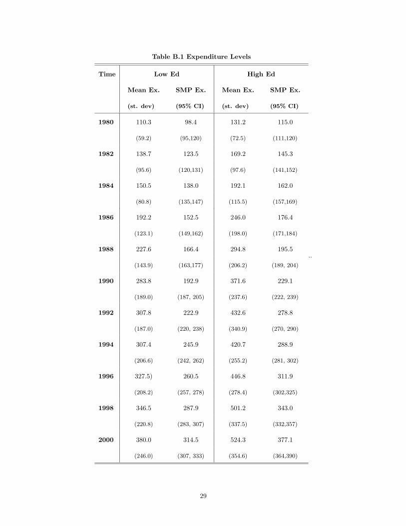
Table B.1 Expenditure Levels

Time Low Ed High Ed

Mean Ex.

(st. dev)

SMP Ex.

(95% CI)

Mean Ex.

(st. dev)

SMP Ex.

(95% CI)

1980 110.3 98.4 131.2 115.0

(59.2) (95,120) (72.5) (111,120)

1982 138.7 123.5 169.2 145.3

(95.6) (120,131) (97.6) (141,152)

1984 150.5 138.0 192.1 162.0

(80.8) (135,147) (115.5) (157,169)

1986 192.2 152.5 246.0 176.4

(123.1) (149,162) (198.0) (171,184)

1988 227.6 166.4 294.8 195.5

(143.9) (163,177) (206.2) (189, 204)

1990 283.8 192.9 371.6 229.1

(189.0) (187, 205) (237.6) (222, 239)

1992 307.8 222.9 432.6 278.8

(187.0) (220, 238) (340.9) (270, 290)

1994 307.4 245.9 420.7 288.9

(206.6) (242, 262) (255.2) (281, 302)

1996 327.5) 260.5 446.8 311.9

(208.2) (257, 278) (278.4) (302,325)

1998 346.5 287.9 501.2 343.0

(220.8) (283, 307) (337.5) (332,357)

2000 380.0 314.5 524.3 377.1

(246.0) (307, 333) (354.6) (364,390)

..

29

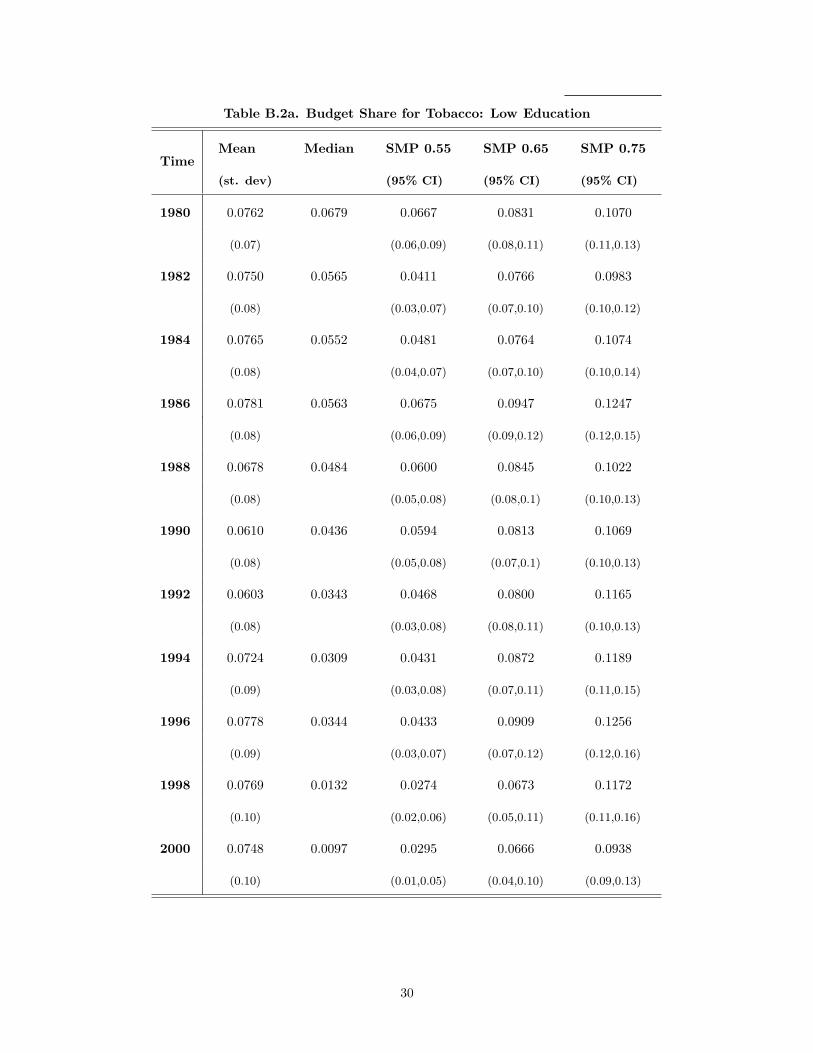
Table B.2a. Budget Share for Tobacco: Low Education

TimeMean

(st. dev)

Median SMP 0.55

(95% CI)

SMP 0.65

(95% CI)

SMP 0.75

(95% CI)

1980 0.0762 0.0679 0.0667 0.0831 0.1070

(0.07) (0.06,0.09) (0.08,0.11) (0.11,0.13)

1982 0.0750 0.0565 0.0411 0.0766 0.0983

(0.08) (0.03,0.07) (0.07,0.10) (0.10,0.12)

1984 0.0765 0.0552 0.0481 0.0764 0.1074

(0.08) (0.04,0.07) (0.07,0.10) (0.10,0.14)

1986 0.0781 0.0563 0.0675 0.0947 0.1247

(0.08) (0.06,0.09) (0.09,0.12) (0.12,0.15)

1988 0.0678 0.0484 0.0600 0.0845 0.1022

(0.08) (0.05,0.08) (0.08,0.1) (0.10,0.13)

1990 0.0610 0.0436 0.0594 0.0813 0.1069

(0.08) (0.05,0.08) (0.07,0.1) (0.10,0.13)

1992 0.0603 0.0343 0.0468 0.0800 0.1165

(0.08) (0.03,0.08) (0.08,0.11) (0.10,0.13)

1994 0.0724 0.0309 0.0431 0.0872 0.1189

(0.09) (0.03,0.08) (0.07,0.11) (0.11,0.15)

1996 0.0778 0.0344 0.0433 0.0909 0.1256

(0.09) (0.03,0.07) (0.07,0.12) (0.12,0.16)

1998 0.0769 0.0132 0.0274 0.0673 0.1172

(0.10) (0.02,0.06) (0.05,0.11) (0.11,0.16)

2000 0.0748 0.0097 0.0295 0.0666 0.0938

(0.10) (0.01,0.05) (0.04,0.10) (0.09,0.13)

30

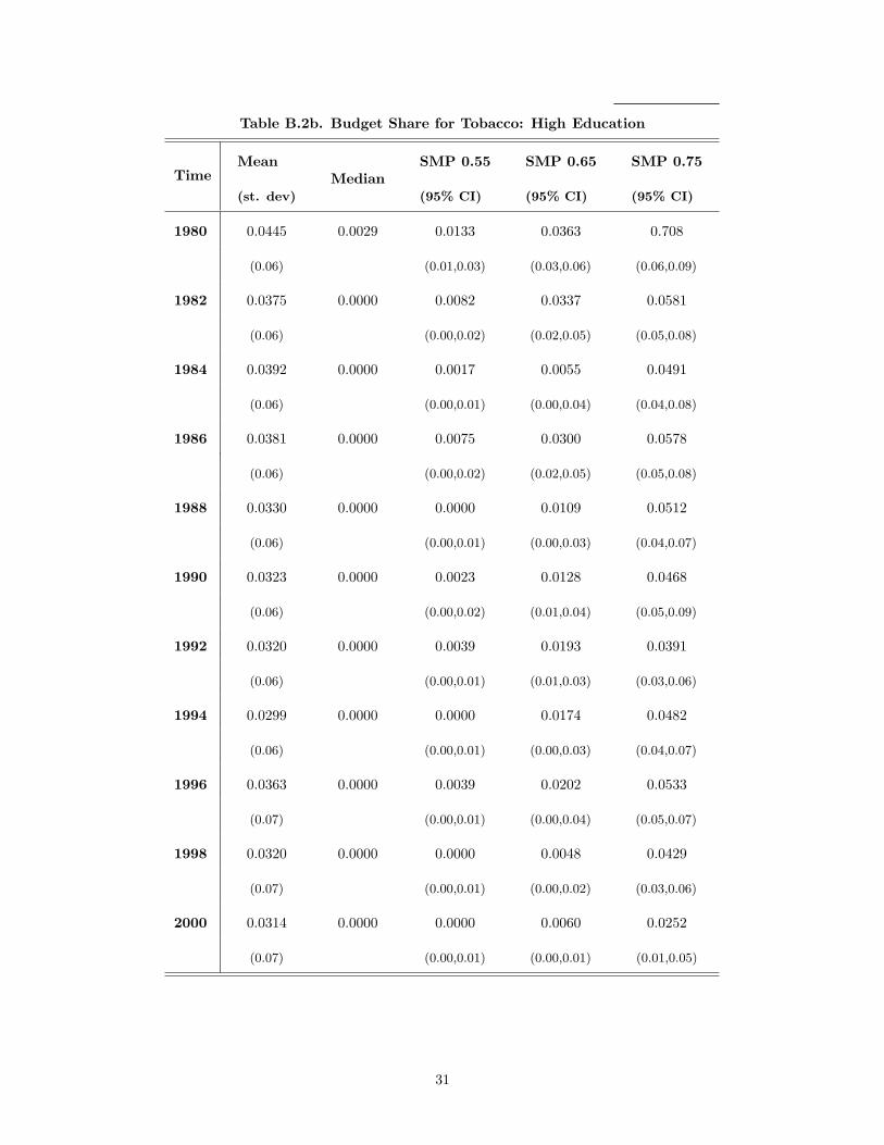
Table B.2b. Budget Share for Tobacco: High Education

TimeMean

(st. dev)

MedianSMP 0.55

(95% CI)

SMP 0.65

(95% CI)

SMP 0.75

(95% CI)

1980 0.0445 0.0029 0.0133 0.0363 0.708

(0.06) (0.01,0.03) (0.03,0.06) (0.06,0.09)

1982 0.0375 0.0000 0.0082 0.0337 0.0581

(0.06) (0.00,0.02) (0.02,0.05) (0.05,0.08)

1984 0.0392 0.0000 0.0017 0.0055 0.0491

(0.06) (0.00,0.01) (0.00,0.04) (0.04,0.08)

1986 0.0381 0.0000 0.0075 0.0300 0.0578

(0.06) (0.00,0.02) (0.02,0.05) (0.05,0.08)

1988 0.0330 0.0000 0.0000 0.0109 0.0512

(0.06) (0.00,0.01) (0.00,0.03) (0.04,0.07)

1990 0.0323 0.0000 0.0023 0.0128 0.0468

(0.06) (0.00,0.02) (0.01,0.04) (0.05,0.09)

1992 0.0320 0.0000 0.0039 0.0193 0.0391

(0.06) (0.00,0.01) (0.01,0.03) (0.03,0.06)

1994 0.0299 0.0000 0.0000 0.0174 0.0482

(0.06) (0.00,0.01) (0.00,0.03) (0.04,0.07)

1996 0.0363 0.0000 0.0039 0.0202 0.0533

(0.07) (0.00,0.01) (0.00,0.04) (0.05,0.07)

1998 0.0320 0.0000 0.0000 0.0048 0.0429

(0.07) (0.00,0.01) (0.00,0.02) (0.03,0.06)

2000 0.0314 0.0000 0.0000 0.0060 0.0252

(0.07) (0.00,0.01) (0.00,0.01) (0.01,0.05)

31