PRESSURE • STRAIN • FORCE
86
http://www.omega.com • e-mail: [email protected] http://www.omega.com • e-mail: [email protected] VOLUME 3 FORCE-RELATED MEASUREMENTS VOLUME 3 FORCE-RELATED MEASUREMENTS PRESSURE • STRAIN • FORCE PRESSURE • STRAIN • FORCE omega.com ® ® The cover is based on an original Norman Rockwell illustration. ©The Curtis Publishing Company.
Transcript of PRESSURE • STRAIN • FORCE

http://www.omega.com • e-mail: [email protected]
http://www.omega.com • e-mail: [email protected]
VOLUME 3FORCE-RELATED MEASUREMENTS
VOLUME 3FORCE-RELATED MEASUREMENTS
PRESSU
RE• S
TRAIN•
FORC
E
PRES
SURE
• STR
AIN• F
ORCE
omega.com®
®
The cover is based on an originalNorman Rockwell illustration.
©The Curtis Publishing Company.

Atmos Bars Dynes/cm2 In of Hg In of H20 K grams/ Lb/in2 psi Lb/ft2 mm of Hg Microns Pascals
(0° C) (4° C) meter2 torr
Atmos
Bars
Dynes/cm2
In of Hg (0°C)
In of H20 (4°C)
K grams/meter2
Lb/in2 psi
Lb/ft2
mm of Hg torr
Microns
Pascals
9.86923 x 10⁻¹
1.01325 x 10⁶
9.86923 x 10⁻⁷
3.34207 x 10⁻²
2.458 x 10⁻³
9.678 x 10⁻⁵
0.068046
1
4.7254 x 10⁻⁴
1.316 x 10⁻³
1.316 x 10⁻⁶
9.869 x 10⁻⁶
750.06 x 10³
0.75006
2.54 x 10⁴
1.868 x 10³
73.558
51.715 x 10³
359.1
1 x 10³
1
7.502
1 x 10⁻¹
10-1
3.386 x 10³
2.491 x 10²
9.8067
6.8948 x 10³
4.788 x 101
1.333 x 10²
1.333 x 10⁻¹
1
750.06
7.5006 x 10⁻⁴
25.400
1.868
7.3558 x 10⁻²
51.715
0.35913
1
10-3
7.502 x 10⁻³
2088.5
2.0885 x 10⁻³
70.726
5.202
0.2048
144.0
1
2.7844
2.7844 x 10⁻³
2.089 x 10⁻²
14.504
1.4504 x 10⁻⁵
0.4912
3.6126 x 10⁻³
1.423 x 10⁻³
1
6.9444 x 10⁻³
1.934 x 10⁻²
1.934 x 10⁻⁵
1.450 x 10⁻⁴
1.0197 x 10⁴
1.0197 x 10⁻²
345.3
25.40
1
7.0306 x 10²
4.882
13.59
13.59 x 10⁻³
1.019 x 10⁻¹
4.01.48
4.0148 x 10⁻⁴
13.60
1
3.937 x 10⁻²
27.68
0.1922
0.5354
5.354 x 10⁻⁴
4.014 x 10⁻³
29.53
29.53 x 10⁻⁵
1
7.355 x 10⁻²
2.896 x 10⁻³
2.036
0.014139
3.937 x 10⁻²
3.937 x 10⁻⁵
2.953 x 10⁻⁴
106
1
3.386 x 10⁻²
2.491 x 10³
98.067
4.78.8
1.333 x 10³
1.333
10
1
10-6
3.3864 x 10⁻²
2.491 x 10⁻³
9.8067 x 10⁻⁵
6.8948 x 10⁻²
6.8948 x 10⁴
1.01325
1.033227 x 10⁴
760 x 103
1.01325 x 10⁵
29.9213
406.8
14.695595
2116.22
760
4.788 x 10⁻⁴
1.333 x 10⁻³
1.333 x 10⁻⁶
10-5
PRESSURE CONVERSION TABLE
GF[(1 + ν)-2Vr(ν - 1)]
-4Vrε = • 1 +
GF[(ν + 1)-Vr(ν - 1)]
-2Vrε =GF(ν + 1)
-2Vrε =
Rg
Rl( ) GF-2Vrε = • 1 +
Rg
Rl( )
VIN
R2
GF(1 + 2Vr)-4Vr
Rl
Rl
Rl
R1
+ + -
-
R3
Rg(ε)
VOUT VIN
R2 Rl
Rl
Rl
R1
+ + -
-
Rg(ε)
Rg Dummy
VOUT
ε = • 1 +Rg
Rl( )
VIN
GF-Vr
-ε
+ε
+ε
-ε
+ + -
- VOUT
ε =
VIN
R2 Rl
Rl
Rl
R1
+ + -
-
Rg(+ε)
Rg(-ε)
VOUT VIN
R2 Rl
Rl
Rl
R1
+ + -
-
Rg(+ε)
Rg(-νε)
VOUT
(AXIAL)
(AXIAL)
(BENDING)
(BENDING)
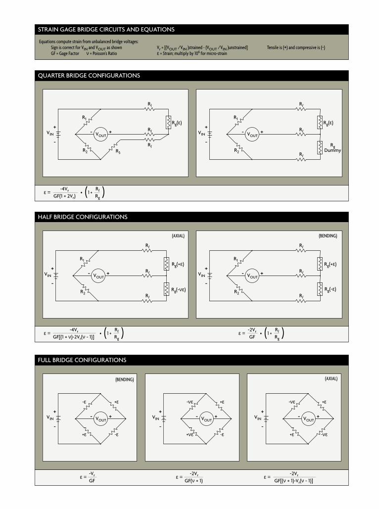
Equations compute strain from unbalanced bridge voltages: Sign is correct for VIN and VOUT as shown GF = Gage Factor ν = Poisson's Ratio
Vr = [(VOUT /VIN )strained - (VOUT /VIN )unstrained] ε = Strain; multiply by 106 for micro-strain
Tensile is (+) and compressive is (-)
VIN
-νε
+νε
+ε
-ε
+ + -
- VOUT VIN
-νε
+ε
+ε
-νε
+ + -
- VOUT
QUARTER BRIDGE CONFIGURATIONS
STRAIN GAGE BRIDGE CIRCUITS AND EQUATIONS
FULL BRIDGE CONFIGURATIONS
HALF BRIDGE CONFIGURATIONS

© 1998 Putman Publishing Company and OMEGA Press LLC.
omega.com®
®
Notice of Intellectual Property Rights
The OMEGA® Handbook Series is based upon originalintellectual property rights that were created anddeveloped by OMEGA. These rights are protectedunder applicable copyright, trade dress, patent andtrademark laws. The distinctive, composite appear-ance of these Handbooks is uniquely identified withOMEGA, including graphics, product identifying pings,paging/section highlights, and layout style. The front,back and inside front cover arrangement is the subjectof a U. S. Patent Pending.

Force-Related MeasurementsA Technical Reference Series Brought to You by OMEGA
33
VOLUME
I N M E A S U R E M E N T A N D C O N T R O L
P R E S S U R E • S T R A I N • W E I G H T • A C C E L E R A T I O N • T O R Q U E
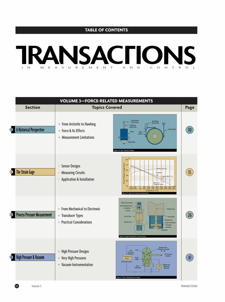
06 Volume 3 TRANSACTIONS
A Historical Perspective1 • From Aristotle to Hawking
• Force & Its Effects
• Measurement Limitations
Figure 1-6: Tank "Staying" Designs
Overhead Structure
Tension Load Cell
Tank Ball Joints
Stay Rods
Stay Rods
Building Structure
The Strain Gage2
10
I N M E A S U R E M E N T A N D C O N T R O L
TABLE OF CONTENTS
VOLUME 3—FORCE-RELATED MEASUREMENTSSection Topics Covered Page
• Sensor Designs
• Measuring Circuits
• Application & Installation
Advance (Cu Ni)
Nichrome
Perc
ent
Cha
nge
In G
auge
Fac
tor
-400 -200 0 200 400 600 800 1000 1200 1400 1600 (-240) (-129) (-18) (93) (204) (315) (426) (538) (649) (760) (871)
120
110
100
90
80
70
Temperature °F (°C)
Karma (Ni Cr +)
Platinum- Tungsten Alloy
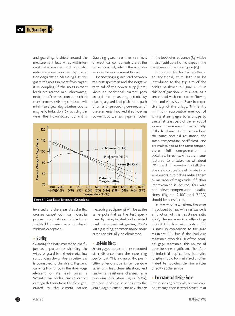
Figure 2-11: Gage Factor Temperature Dependence
15
Process Pressure Measurement3
• From Mechanical to Electronic
• Transducer Types
• Practical Considerations
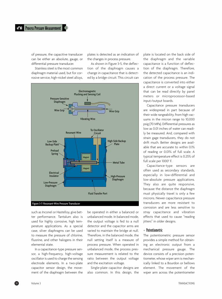
Element Lead
Seal Surface
Preload Screw
Quartz Crystal (2)
Electrode
End Piece
Diaphragm
Electrical Connector
Shrink Tubing Grooves
IC Amplifier
5/16 Hex
5/16-24 Thd.
Element Lead
Figure 3-8: Typical Piezoelectric Pressure Sensor
26
High Pressure & Vacuum4
• High Pressure Designs
• Very High Pressures
• Vacuum Instrumentation
Figure 4-7: Hot-Cathode Vacuum Gauge
IonsPositive Ion
Collector Anode @ - 30
To Vacuum System
Meter For Electron (10mA)
Grid + 150V
(100 mA/torr)
Hot Cathode
++
Ion Current
Detector
-
++
+ ++
- - ----
- -
Indicating Meter 41
TRANSACTIONS Volume 3 07
Pressure Gauges & Switches5
• Pressure Gauge Designs
• Protective Accessories
• Pressure Switches
Section Topics Covered Page
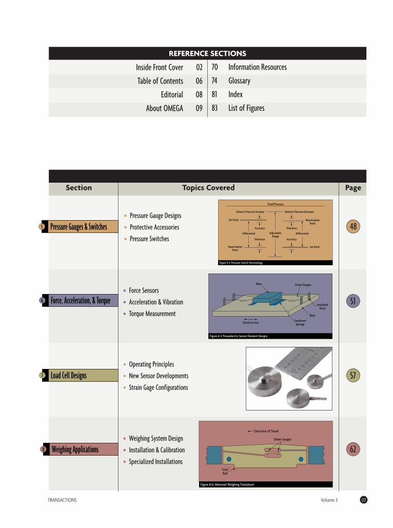
Figure 5-3: Pressure Switch Terminology
Proof Pressure
Reactivation Point
Reactivation Point
Set Point
Set Point
DifferentialDifferential
Accuracy
Accuracy Tolerance
Tolerance
Adjustable Range
Detects Pressure DecreaseDetects Pressure Increase
Force, Acceleration, & Torque6
48
Load Cell Designs7
• Force Sensors
• Acceleration & Vibration
• Torque Measurement
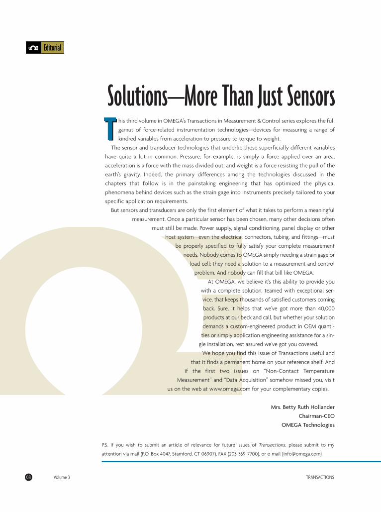
Mass Strain Gauges
Insulated Posts
Base
Cantilever SpringsSensitive Axis
Figure 6-3: Piezoelectric Sensor Element Designs
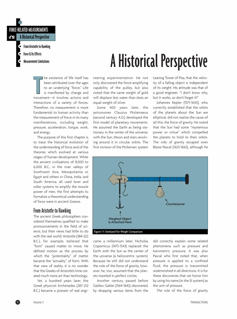
• Operating Principles
• New Sensor Developments
• Strain Gage Configurations
Inside Front Cover 02
Table of Contents 06
Editorial 08
About OMEGA 09
51
57
REFERENCE SECTIONS
70 Information Resources
74 Glossary
81 Index
83 List of Figures
Weighing Applications 8
• Weighing System Design
• Installation & Calibration
• Specialized Installations
62
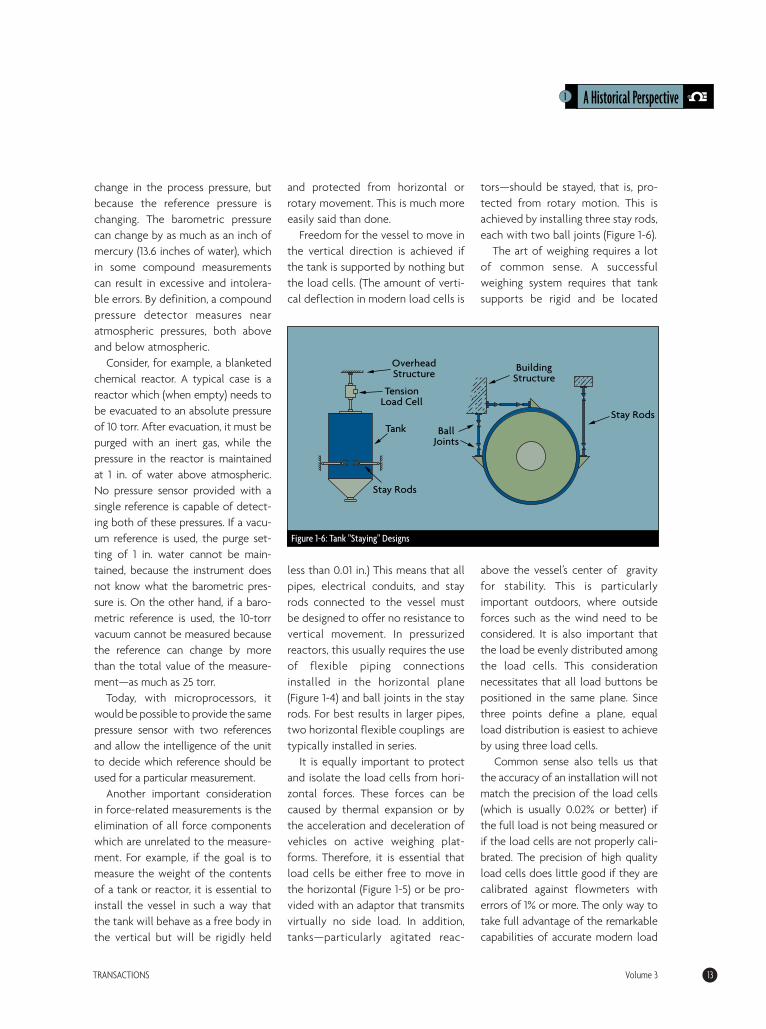
Figure 8-6: Monorail Weighing Transducer
Strain Gauges
Direction of Travel
"Live" Rail
Editorial
08 Volume 3 TRANSACTIONS
Solutions–More Than Just SensorsT his third volume in OMEGA’s Transactions in Measurement & Control series explores the full
gamut of force-related instrumentation technologies—devices for measuring a range of
kindred variables from acceleration to pressure to torque to weight.
The sensor and transducer technologies that underlie these superficially different variables
have quite a lot in common. Pressure, for example, is simply a force applied over an area,
acceleration is a force with the mass divided out, and weight is a force resisting the pull of the
earth’s gravity. Indeed, the primary differences among the technologies discussed in the
chapters that follow is in the painstaking engineering that has optimized the physical
phenomena behind devices such as the strain gage into instruments precisely tailored to your
specific application requirements.
But sensors and transducers are only the first element of what it takes to perform a meaningful
measurement. Once a particular sensor has been chosen, many other decisions often
must still be made. Power supply, signal conditioning, panel display or other
host system—even the electrical connectors, tubing, and fittings—must
be properly specified to fully satisfy your complete measurement
needs. Nobody comes to OMEGA simply needing a strain gage or
load cell; they need a solution to a measurement and control
problem. And nobody can fill that bill like OMEGA.
At OMEGA, we believe it’s this ability to provide you
with a complete solution, teamed with exceptional ser-
vice, that keeps thousands of satisfied customers coming
back. Sure, it helps that we’ve got more than 40,000
products at our beck and call, but whether your solution
demands a custom-engineered product in OEM quanti-
ties or simply application engineering assistance for a sin-
gle installation, rest assured we’ve got you covered.
We hope you find this issue of Transactions useful and
that it finds a permanent home on your reference shelf. And
if the first two issues on “Non-Contact Temperature
Measurement” and “Data Acquisition” somehow missed you, visit
us on the web at www.omega.com for your complementary copies.
T
Mrs. Betty Ruth Hollander
Chairman-CEO
OMEGA Technologies
P.S. If you wish to submit an article of relevance for future issues of Transactions, please submit to my
attention via mail (P.O. Box 4047, Stamford, CT 06907), FAX (203-359-7700), or e-mail ([email protected]).

About OMEGA
TRANSACTIONS Volume 3 09
OMEGA’s Transactions in Measurement & Control series, as well as our legendary set of handbooks and
encyclopedias, are designed to provide at-your-fingertips access to the technical information you need
to help meet your measurement and control requirements. But when your needs exceed the printed
word—when technical assistance is required to select among alternative products, or when no “off-the-shelf”
product seems to fill the bill—we hope you’ll turn to OMEGA. There is no advertising or
promotional material in the Transactions series. There will be none.
Our people, our facilities, and our commitment to customer service set the standard
for control and instrumentation. A sampler of our comprehensive resources and
capabilities:
• OMEGA’s commitment to leading-edge research and development and
state-of-the-art manufacturing keeps us firmly at the forefront of technology.
OMEGA’s Development and Engineering Center, located on our Stamford, CT,
campus, is home to OMEGA’s design and engineering laboratories. All product
designs are tested and perfected here prior to marketing. This facility houses
OMEGA’s metrology lab and other quality control facilities. The testing that takes place here assures
that you receive the best products for your applications.
• On the manufacturing side, our Bridgeport, NJ, vertically integrated manufacturing facility near
Philadelphia houses advanced thermocouple wire production equipment along with a host of other com-
puterized CNC milling machines, injection molding equipment, screw machines, braiders, extruders,
punch presses and much, much more.
• If our broad range of standard products doesn’t quite match your needs, OMEGA is proud to offer the
most sophisticated and extensive custom engineering capabilities in the process measurement and control
industry. Whether you need a simple modification of a standard product or complete customized system,
OMEGA can accommodate your special request. Free CAD drawings also are supplied with customized product
orders, or a new design can be built to your specifications with no obligation.
• We believe in active versus reactive customer service. To complement our current business and
manufacturing operations, OMEGA continues to strive toward new levels of quality by pursuing ISO 9000
quality standards. This systematic approach to quality strengthens OMEGA’s competitive edge. Our
calibration services and quality control test center are trustworthy resources that help satisfy our customers’
needs for accuracy on an initial and ongoing basis.
• The company’s technical center welcomes many corporate groups of engineers and scientists who
turn to OMEGA for training. Our 140-seat auditorium, equipped with the latest in multimedia presentation
technologies, provides an ideal learning environment for training tailored to your company’s needs—from
basic refreshers to in-depth courses.
In short, it is our commitment to quality instrumentation and exceptional customer service that remains
the cornerstone of our success. OMEGA’s priority is clear: we exist to facilitate solutions to your needs.
For more information about Transactions or OMEGA Technologies, look us up on the Internet at
www.omega.com.
Exceeding Your ExpectationsO
The existence of life itself hasbeen attributed over the agesto an underlying “force.” Lifeis manifested by change and
movement—it involves actions andinteractions of a variety of forces.Therefore, no measurement is morefundamental to human activity thanthe measurement of force in its manymanifestations, including weight,pressure, acceleration, torque, work,and energy.
The purpose of this first chapter isto trace the historical evolution ofthe understanding of force and of thetheories which evolved at variousstages of human development. Whilethe ancient civilizations of 8,000 to6,000 B.C., in the river valleys ofSouthwest Asia, Mesopotamia orEgypt and others in China, India, andSouth America, all used lever androller systems to amplify the musclepower of men, the first attempts toformalize a theoretical understandingof force were in ancient Greece.
From Aristotle to HawkingThe ancient Greek philosophers con-sidered themselves qualified to makepronouncements in the field of sci-ence, but their views had little to dowith the real world. Aristotle (384-322B.C.), for example, believed that“form” caused matter to move. Hedefined motion as the process bywhich the “potentiality” of matterbecame the “actuality” of form. Withthat view of reality, it is no wonderthat the Greeks of Aristotle’s time cre-ated much more art than technology.
Yet, a hundred years later, theGreek physicist Archimedes (287-212B.C.) became a pioneer of real engi-
neering experimentation. He notonly discovered the force-amplifyingcapability of the pulley, but alsonoted that the same weight of goldwill displace less water than does anequal weight of silver.
Some 400 years later, theastronomer Clausius Ptolemaeus(second century A.D.) developed thefirst model of planetary movements.He assumed the Earth as being sta-tionary in the center of the universe,with the Sun, Moon and stars revolv-ing around it in circular orbits. Thefirst revision of the Ptolemaic system
came a millennium later; NicholasCopernicus (1473-1543) replaced theEarth with the Sun as the center ofthe universe (a heliocentric system).Because he still did not understandthe role of the force of gravity, how-ever, he, too, assumed that the plan-ets traveled in perfect circles.
Another century passed beforeGalileo Galilei (1564-1642) discovered,by dropping various items from the
Leaning Tower of Pisa, that the veloc-ity of a falling object is independentof its weight. His attitude was that ofa good engineer: “I don’t know why,but it works, so don’t forget it!”
Johannes Kepler (1571-1630), whocorrectly established that the orbitsof the planets about the Sun areelliptical, did not realize the cause ofall this: the force of gravity. He notedthat the Sun had some “mysteriouspower or virtue” which compelledthe planets to hold to their orbits.The role of gravity escaped evenBlaise Pascal (1623-1662), although he
did correctly explain some relatedphenomena such as pressure andbarometric pressure. It was alsoPascal who first noted that, whenpressure is applied to a confinedfluid, the pressure is transmittedundiminished in all directions. It is forthese discoveries that we honor himby using his name (in the SI system) asthe unit of pressure.
The role of the force of gravity
10 Volume 3 TRANSACTIONS
From Aristotle to Hawking
Force & Its Effects
Measurement Limitations
FORCE-RELATED MEASUREMENTSA Historical Perspective
1
TA Historical Perspective
Figure 1-1: Steelyard for Weight Comparison
Counterpoise
Weighed Object Is Attached Here

was first fully understood by Sir IsaacNewton (1642-1727). His law of uni-versal gravitation explained both thefall of bodies on Earth and themotion of heavenly bodies. He provedthat gravitational attraction existsbetween any two material objects. Healso noted that this force is directlyproportional to the product of themasses of the objects and inverselyproportional to the square of the
distance between them. On the Earth’ssurface, the measure of the force ofgravity on a given body is its weight.The strength of the Earth’s gravitation-al field (g) varies from 9.832 m/sec2 atsea level at the poles to 9.78 m/sec2 atsea level at the Equator.
Newton summed up his under-standing of motion in three laws:
1) The law of inertia: A body dis-plays an inherent resistance tochanging its speed or direction. Botha body at rest and a body in motiontend to remain so.
2) The law of acceleration: Mass (m)is a numerical measure of inertia. Theacceleration (a) resulting from a force(F) acting on a mass can be expressedin the equation a = F/m; therefore, itcan be seen that the greater the mass(inertia) of a body, the less accelera-tion will result from the application
of the same amount of force upon it.3) For every action, there is an
equal and opposite reaction.After Newton, progress in under-
standing force-related phenomenaslowed. James Prescott Joule (1818-1889) determined the relationshipbetween heat and the variousmechanical forms of energy. He alsoestablished that energy cannot belost, only transformed (the principleof conservation of energy), definedpotential energy (the capacity fordoing work), and established thatwork performed (energy expended)is the product of the amount offorce applied and the distance trav-eled. In recognition of his contribu-tions, the unit of work and energy inthe SI system is called the joule.
Albert Einstein (1879-1955) con-tributed another quantum jump in ourunderstanding of force-related phe-nomena. He established the speed oflight (c = 186,000 miles/sec) as themaximum theoretical speed that anyobject with mass can travel, and thatmass (m) and energy (e) are equivalentand interchangeable: e = mc2.
Einstein’s theory of relativity cor-rected the discrepancies in Newton’stheory and explained them geomet-rically: concentrations of mattercause a curvature in the space-timecontinuum, resulting in “gravitywaves.” While making enormous con-tributions to the advancement of sci-ence, the goal of developing a uni-fied field theory (a single set of lawsthat explain gravitation, electromag-netism, and subatomic phenomena)eluded Einstein.
Edwin Powell Hubble (1889-1953)improved our understanding of theuniverse, noting that it looks thesame from all positions, and in alldirections, and that distancesbetween galaxies are continuously
increasing. According to Hubble, thisexpansion of the universe started 10to 20 billion years ago with a “bigbang,” and the space-time fabricwhich our universe occupies contin-ues to expand.
Carlo Rubbia (1934- ) and Simon vander Meer (1925- ) further advanced ourunderstanding of force by discoveringthe subatomic W and Z particles whichconvey the “weak force” of atomicdecay. Stephen Hawking (1952- )advanced our understanding even fur-ther with his theory of strings. Stringscan be thought of as tiny vibratingloops from which both matter andenergy derive. His theory holds thepromise of unifying Einstein’s theory ofrelativity, which explains gravity andthe forces acting in the macro world,with quantum theory, which describesthe forces acting on the atomic andsubatomic levels.
Force & Its Effects Force is a quantity capable of chang-ing the size, shape, or motion of anobject. It is a vector quantity and,as such, it has both direction andmagnitude. In the SI system, the
magnitude of a force is measured inunits called newtons, and in poundsin the British/American system. If a
1 A Historical Perspective
TRANSACTIONS Volume 3 11
Figure 1-2: Vacuum Reference Gauge
Process Connection
Force Bar
Bellows
Fulcrum & Seal
Vacuum Reference
Figure 1-3: Atmospheric Reference Gauge
Process Connection
Force Bar
Bellows
Stop
Fulcrum & Seal
Atmospheric Reference

body is in motion, the energy of thatmotion can be quantified as themomentum of the object, the productof its mass and its velocity. If a body isfree to move, the action of a force will
change the velocity of the body.There are four basic forces in
nature: gravitational, magnetic, strongnuclear, and weak nuclear forces. Theweakest of the four is the gravitation-al force. It is also the easiest toobserve, because it acts on all matterand it is always attractive, while hav-ing an infinite range. Its attractiondecreases with distance, but is alwaysmeasurable. Therefore, positional“equilibrium” of a body can only beachieved when gravitational pull isbalanced by another force, such as theupward force exerted on our feet bythe earth’s surface.
Pressure is the ratio between aforce acting on a surface and the areaof that surface. Pressure is measuredin units of force divided by area:pounds per square inch (psi) or, in theSI system, newtons per square meter,or pascals. When an external stress(pressure) is applied to an objectwith the intent to cause a reductionin its volume, this process is calledcompression. Most liquids and solidsare practically incompressible, whilegases are not.
The First Gas Law, called Boyle’slaw, states that the pressure and vol-ume of a gas are inversely propor-tional to one another: PV = k, whereP is pressure, V is volume and k is a
constant of proportionality. TheSecond Gas Law, Charles’ Law, statesthat the volume of an enclosed gas isdirectly proportional to its tempera-ture: V = kT, where T is its absolutetemperature. And, according to theThird Gas Law, the pressure of a gas isdirectly proportional to its absolutetemperature: P = kT.
Combining these three relation-ships yields the ideal gas law: PV =kT. This approximate relationshipholds true for many gases at rela-tively low pressures (not too closeto the point where liquificationoccurs) and high temperatures (nottoo close to the point where con-densation is imminent).
Measurement LimitationsOne of the basic limitations of allmeasurement science, or metrology,is that all measurements are relative.Therefore, all sensors contain a refer-ence point against which the quanti-ty to be measured must be com-pared. The steelyard was one ofmankind’s first relative sensors,invented to measure the weight of an
object (Figure 1-1). It is a beam sup-ported from hooks (A or B), while theobject to be weighed is attached tothe shorter arm of the lever and acounterpoise is moved along thelonger arm until balance is estab-lished. The precision of such weightscales depends on the precision ofthe reference weight (the counter-poise) and the accuracy with which itis positioned.
Similarly, errors in pressure mea-surement are as often caused byinaccurate reference pressures asthey are by sensor inaccuracies. Ifabsolute pressure is to be detected,the reference pressure (theoretically)should be zero—a complete vacuum.In reality, a reference chamber can-not be evacuated to absolute zero(Figure 1-2), but only to a few thou-sandths of a millimeter of mercury(torr). This means that a nonzeroquantity is used as a zero reference.Therefore, the higher that referencepressure, the greater the resultingerror. Another source of error inabsolute pressure measurement is theloss of the vacuum reference due to
the intrusion of air. In the case of “gauge” pressure
measurement, the reference is atmos-pheric pressure, which is itself vari-able (Figure 1-3). Thus, sensor outputcan change not because there is a
A Historical Perspective 1
12 Volume 3 TRANSACTIONS
Figure 1-4: Flexible Load-Cell Connections
Normal Angular Misalignment
Parallel Misalignment
Figure 1-5: Typical Load Cell Installation
change in the process pressure, butbecause the reference pressure ischanging. The barometric pressurecan change by as much as an inch ofmercury (13.6 inches of water), whichin some compound measurementscan result in excessive and intolera-ble errors. By definition, a compoundpressure detector measures nearatmospheric pressures, both aboveand below atmospheric.
Consider, for example, a blanketedchemical reactor. A typical case is areactor which (when empty) needs tobe evacuated to an absolute pressureof 10 torr. After evacuation, it must bepurged with an inert gas, while thepressure in the reactor is maintainedat 1 in. of water above atmospheric.No pressure sensor provided with asingle reference is capable of detect-ing both of these pressures. If a vacu-um reference is used, the purge set-ting of 1 in. water cannot be main-tained, because the instrument doesnot know what the barometric pres-sure is. On the other hand, if a baro-metric reference is used, the 10-torrvacuum cannot be measured becausethe reference can change by morethan the total value of the measure-ment—as much as 25 torr.
Today, with microprocessors, itwould be possible to provide the samepressure sensor with two referencesand allow the intelligence of the unitto decide which reference should beused for a particular measurement.
Another important considerationin force-related measurements is theelimination of all force componentswhich are unrelated to the measure-ment. For example, if the goal is tomeasure the weight of the contentsof a tank or reactor, it is essential toinstall the vessel in such a way thatthe tank will behave as a free body inthe vertical but will be rigidly held
and protected from horizontal orrotary movement. This is much moreeasily said than done.
Freedom for the vessel to move inthe vertical direction is achieved ifthe tank is supported by nothing butthe load cells. (The amount of verti-cal deflection in modern load cells is
less than 0.01 in.) This means that allpipes, electrical conduits, and stayrods connected to the vessel mustbe designed to offer no resistance tovertical movement. In pressurizedreactors, this usually requires the useof flexible piping connectionsinstalled in the horizontal plane(Figure 1-4) and ball joints in the stayrods. For best results in larger pipes,two horizontal flexible couplings aretypically installed in series.
It is equally important to protectand isolate the load cells from hori-zontal forces. These forces can becaused by thermal expansion or bythe acceleration and deceleration ofvehicles on active weighing plat-forms. Therefore, it is essential thatload cells be either free to move inthe horizontal (Figure 1-5) or be pro-vided with an adaptor that transmitsvirtually no side load. In addition,tanks—particularly agitated reac-
tors—should be stayed, that is, pro-tected from rotary motion. This isachieved by installing three stay rods,each with two ball joints (Figure 1-6).
The art of weighing requires a lotof common sense. A successfulweighing system requires that tanksupports be rigid and be located
above the vessel’s center of gravityfor stability. This is particularlyimportant outdoors, where outsideforces such as the wind need to beconsidered. It is also important thatthe load be evenly distributed amongthe load cells. This considerationnecessitates that all load buttons bepositioned in the same plane. Sincethree points define a plane, equalload distribution is easiest to achieveby using three load cells.
Common sense also tells us thatthe accuracy of an installation will notmatch the precision of the load cells(which is usually 0.02% or better) ifthe full load is not being measured orif the load cells are not properly cali-brated. The precision of high qualityload cells does little good if they arecalibrated against flowmeters witherrors of 1% or more. The only way totake full advantage of the remarkablecapabilities of accurate modern load
1 A Historical Perspective
TRANSACTIONS Volume 3 13
Figure 1-6: Tank "Staying" Designs
Overhead Structure
Tension Load Cell
Tank Ball Joints
Stay Rods
Stay Rods
Building Structure
cells is to zero and calibrate the sys-tem using precision dead weights. It isalso important to remember thatdead weights can only be attached toa reactor if hooks or platforms areprovided for them.
Range considerations also areimportant because load cells are per-cent-of-full-scale devices. This meansthat the absolute error correspondingto, say, 0.02% is a function of the totalweight being measured. If the totalweight is 100,000 pounds, theabsolute error is 20 pounds. But if oneneeds to charge a batch of 100 poundsof catalyst into that same reactor, theerror will be 20%, not 0.02%. T
A Historical Perspective 1
14 Volume 3 TRANSACTIONS
References & Further Reading• Black Holes and Baby Universes and Other Essays, Stephen Hawking,
Bantam Books, 1993.• Instrument Engineers’ Handbook, Bela Liptak, CRC Press LLC, 1995.• Instrumentation Reference Book, 2nd Edition, B.E. Noltingk, Butterworth-
Heinemann, 1995. • Marks’ Standard Handbook for Mechanical Engineers, 10th Edition,
Eugene A. Avallone and Theodore Baumeister, McGraw-Hill, 1996.• McGraw-Hill Concise Encyclopedia of Science and Technology, McGraw-
Hill, 1998.• Perry’s Chemical Engineers’ Handbook, 7th Edition, Robert H. Perry, Don
W. Green, and James O. Maloney, McGraw-Hill, 1997. • Process Control Systems: Application, Design, and Tuning, 4th Edition, F.
Greg Shinskey, McGraw Hill, 1996.• Van Nostrand’s Scientific Encyclopedia, Douglas M. Considine and Glenn
D. Considine, Van Nostrand, 1997.
When external forces areapplied to a stationaryobject, stress and strainare the result. Stress is
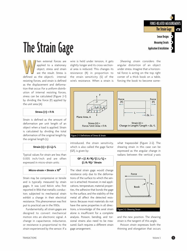
defined as the object’s internalresisting forces, and strain is definedas the displacement and deforma-tion that occur. For a uniform distrib-ution of internal resisting forces,stress can be calculated (Figure 2-1)by dividing the force (F) applied bythe unit area (A):
Stress (σ) = F/A
Strain is defined as the amount ofdeformation per unit length of anobject when a load is applied. Strainis calculated by dividing the totaldeformation of the original length bythe original length (L):
Strain (ε) = (∆ L)/L
Typical values for strain are less than0.005 inch/inch and are oftenexpressed in micro-strain units:
Micro-strain = Strain x 106
Strain may be compressive or tensileand is typically measured by straingages. It was Lord Kelvin who firstreported in 1856 that metallic conduc-tors subjected to mechanical strainexhibit a change in their electricalresistance. This phenomenon was firstput to practical use in the 1930s.
Fundamentally, all strain gages aredesigned to convert mechanicalmotion into an electronic signal. Achange in capacitance, inductance,or resistance is proportional to thestrain experienced by the sensor. If a
wire is held under tension, it getsslightly longer and its cross-section-al area is reduced. This changes itsresistance (R) in proportion tothe strain sensitivity (S) of thewire’s resistance. When a strain is
introduced, the strain sensitivity,which is also called the gage factor(GF), is given by:
GF = (∆ R/R)/(∆ L/L) = (∆ R/R)/ Strain
The ideal strain gage would changeresistance only due to the deforma-tions of the surface to which the sen-sor is attached. However, in real appli-cations, temperature, material proper-ties, the adhesive that bonds the gageto the surface, and the stability of themetal all affect the detected resis-tance. Because most materials do nothave the same properties in all direc-tions, a knowledge of the axial strainalone is insufficient for a completeanalysis. Poisson, bending, and tor-sional strains also need to be mea-sured. Each requires a different straingage arrangement.
Shearing strain considers theangular distortion of an objectunder stress. Imagine that a horizon-tal force is acting on the top rightcorner of a thick book on a table,forcing the book to become some-
what trapezoidal (Figure 2-2). Theshearing strain in this case can beexpressed as the angular change inradians between the vertical y-axis
and the new position. The shearingstrain is the tangent of this angle.
Poisson strain expresses both thethinning and elongation that occurs
TRANSACTIONS Volume 3 15
W
Figure 2-1: Definitions of Stress & Strain
Plane Area, A
Force (F)
Force (F)
L
F
∆L
Stress (σ) = Force/Unit Area = F/A
Strain (ε) = Change in Length/Length = ∆L/L
Figure 2-2: Shearing Strain
Force
γBook
Sensor Designs
Measuring Circuits
Application & Installation
FORCE-RELATED MEASUREMENTSThe Strain Gage
2
The Strain Gage
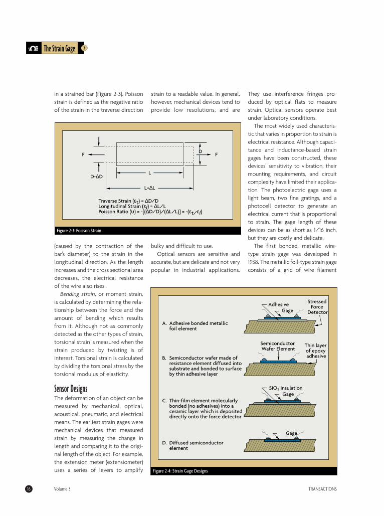
in a strained bar (Figure 2-3). Poissonstrain is defined as the negative ratioof the strain in the traverse direction
(caused by the contraction of thebar’s diameter) to the strain in thelongitudinal direction. As the lengthincreases and the cross sectional areadecreases, the electrical resistanceof the wire also rises.
Bending strain, or moment strain,is calculated by determining the rela-tionship between the force and theamount of bending which resultsfrom it. Although not as commonlydetected as the other types of strain,torsional strain is measured when thestrain produced by twisting is ofinterest. Torsional strain is calculatedby dividing the torsional stress by thetorsional modulus of elasticity.
Sensor DesignsThe deformation of an object can bemeasured by mechanical, optical,acoustical, pneumatic, and electricalmeans. The earliest strain gages weremechanical devices that measuredstrain by measuring the change inlength and comparing it to the origi-nal length of the object. For example,the extension meter (extensiometer)uses a series of levers to amplify
strain to a readable value. In general,however, mechanical devices tend toprovide low resolutions, and are
bulky and difficult to use. Optical sensors are sensitive and
accurate, but are delicate and not verypopular in industrial applications.
They use interference fringes pro-duced by optical flats to measurestrain. Optical sensors operate bestunder laboratory conditions.
The most widely used characteris-tic that varies in proportion to strain iselectrical resistance. Although capaci-tance and inductance-based straingages have been constructed, thesedevices’ sensitivity to vibration, theirmounting requirements, and circuitcomplexity have limited their applica-tion. The photoelectric gage uses alight beam, two fine gratings, and aphotocell detector to generate anelectrical current that is proportionalto strain. The gage length of thesedevices can be as short as 1/16 inch,but they are costly and delicate.
The first bonded, metallic wire-type strain gage was developed in1938. The metallic foil-type strain gageconsists of a grid of wire filament
The Strain Gage 2
16 Volume 3 TRANSACTIONS
Figure 2-3: Poisson Strain
Traverse Strain (εt) = ∆D/D Longitudinal Strain (εl) = ∆L/L Poisson Ratio (υ) = -[(∆D/D)/(∆L/L)] = -(εt/εl)
D-∆D
L+∆L
F
L
FD
Figure 2-4: Strain Gage Designs
A. Adhesive bonded metallic foil element
AdhesiveGage
Gage
Semiconductor Wafer Element
SiO2 insulation
Thin layer of epoxy adhesive
Stressed Force
Detector
B. Semiconductor wafer made of resistance element diffused into substrate and bonded to surface by thin adhesive layer
C. Thin-film element molecularly bonded (no adhesives) into a ceramic layer which is deposited directly onto the force detector
D. Diffused semiconductor element
Gage
(a resistor) of approximately 0.001 in.(0.025 mm) thickness, bonded directlyto the strained surface by a thin layerof epoxy resin (Figure 2-4A). When aload is applied to the surface, theresulting change in surface length iscommunicated to the resistor and thecorresponding strain is measured interms of the electrical resistance ofthe foil wire, which varies linearly withstrain. The foil diaphragm and theadhesive bonding agent must worktogether in transmitting the strain,while the adhesive must also serve asan electrical insulator between thefoil grid and the surface.
When selecting a strain gage, onemust consider not only the straincharacteristics of the sensor, but alsoits stability and temperature sensitiv-ity. Unfortunately, the most desirablestrain gage materials are also sensitiveto temperature variations and tend tochange resistance as they age. Fortests of short duration, this may notbe a serious concern, but for continu-ous industrial measurement, onemust include temperature and driftcompensation.
Each strain gage wire material hasits characteristic gage factor, resis-tance, temperature coefficient ofgage factor, thermal coefficient ofresistivity, and stability. Typical mate-rials include Constantan (copper-nick-el alloy), Nichrome V (nickel-chromealloy), platinum alloys (usually tung-sten), Isoelastic (nickel-iron alloy), orKarma-type alloy wires (nickel-chrome alloy), foils, or semiconductormaterials. The most popular alloysused for strain gages are copper-nick-el alloys and nickel-chromium alloys.
In the mid-1950s, scientists at BellLaboratories discovered the piezore-sistive characteristics of germaniumand silicon. Although the materialsexhibited substantial nonlinearity
and temperature sensitivity, they hadgage factors more than fifty times,and sensitivity more than a 100times, that of metallic wire or foilstrain gages. Silicon wafers are alsomore elastic than metallic ones.After being strained, they returnmore readily to their original shapes.
Around 1970, the first semiconduc-tor (silicon) strain gages were devel-oped for the automotive industry. Asopposed to other types of straingages, semiconductor strain gagesdepend on the piezoresistive effectsof silicon or germanium and measure
the change in resistance with stressas opposed to strain. The semicon-ductor bonded strain gage is a waferwith the resistance element diffusedinto a substrate of silicon. The waferelement usually is not provided witha backing, and bonding it to thestrained surface requires great care asonly a thin layer of epoxy is used toattach it (Figure 2-4B). The size ismuch smaller and the cost muchlower than for a metallic foil sensor.The same epoxies that are used to
attach foil gages also are used tobond semiconductor gages.
While the higher unit resistanceand sensitivity of semiconductorwafer sensors are definite advan-tages, their greater sensitivity totemperature variations and tendencyto drift are disadvantages in compar-ison to metallic foil sensors. Anotherdisadvantage of semiconductorstrain gages is that the resistance-to-strain relationship is nonlinear,varying 10-20% from a straight-lineequation. With computer-controlledinstrumentation, these limitations
can be overcome through softwarecompensation.
A further improvement is the thin-film strain gage that eliminates theneed for adhesive bonding (Figure 2-4C). The gage is produced by firstdepositing an electrical insulation(typically a ceramic) onto thestressed metal surface, and thendepositing the strain gage onto thisinsulation layer. Vacuum depositionor sputtering techniques are used tobond the materials molecularly.
2 The Strain Gage
TRANSACTIONS Volume 3 17
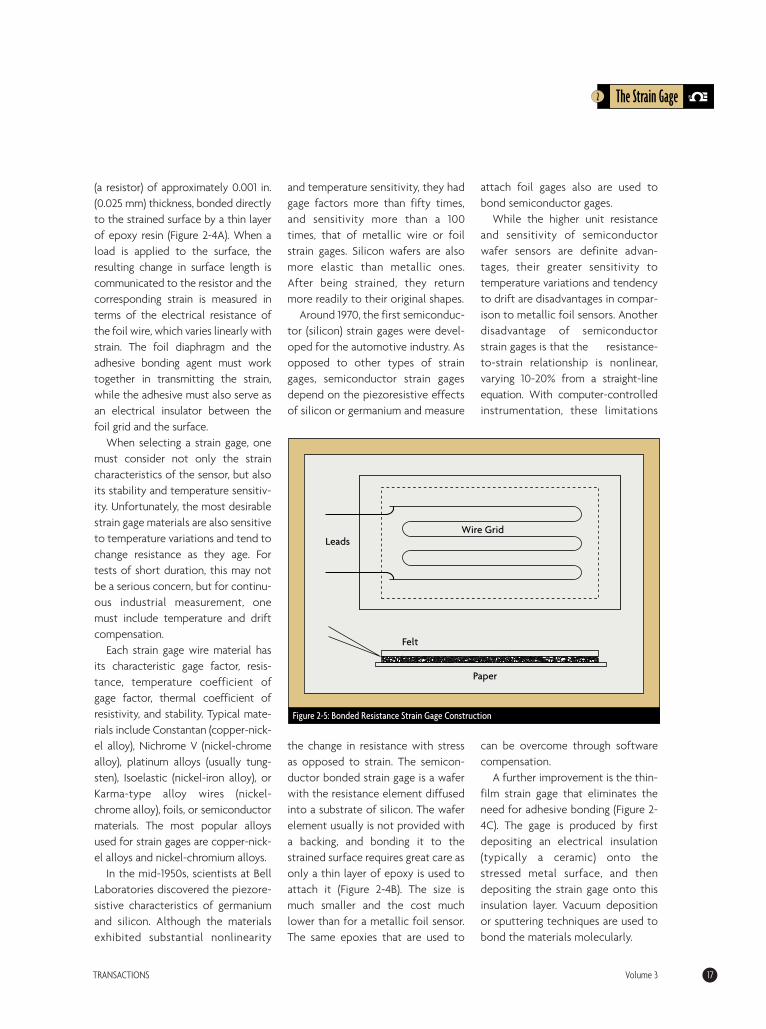
Figure 2-5: Bonded Resistance Strain Gage Construction
Wire Grid
Felt
Leads
Paper
Because the thin-film gage is mole-cularly bonded to the specimen, theinstallation is much more stable andthe resistance values experience lessdrift. Another advantage is that thestressed force detector can be a
metallic diaphragm or beam with adeposited layer of ceramic insulation.
Diffused semiconductor straingages represent a further improve-ment in strain gage technologybecause they eliminate the need forbonding agents. By eliminating bond-ing agents, errors due to creep andhysteresis also are eliminated. The dif-fused semiconductor strain gage usesphotolithography masking techniquesand solid-state diffusion of boron tomolecularly bond the resistance ele-ments. Electrical leads are directlyattached to the pattern (Figure 2-4D).
The diffused gage is limited to
moderate-temperature applicationsand requires temperature compensa-tion. Diffused semiconductors oftenare used as sensing elements in pres-sure transducers. They are small,inexpensive, accurate and repeatable,
provide a wide pressure range, andgenerate a strong output signal. Theirlimitations include sensitivity toambient temperature variations,which can be compensated for inintelligent transmitter designs.
In summary, the ideal strain gage issmall in size and mass, low in cost,easily attached, and highly sensitiveto strain but insensitive to ambientor process temperature variations.
• Bonded Resistance GagesThe bonded semiconductor straingage was schematically described inFigures 2-4A and 2-4B. These devices
represent a popular method of mea-suring strain. The gage consists of agrid of very fine metallic wire, foil, orsemiconductor material bonded tothe strained surface or carrier matrixby a thin insulated layer of epoxy(Figure 2-5). When the carrier matrixis strained, the strain is transmittedto the grid material through theadhesive. The variations in the elec-trical resistance of the grid are mea-sured as an indication of strain. Thegrid shape is designed to providemaximum gage resistance whilekeeping both the length and width ofthe gage to a minimum.
Bonded resistance strain gageshave a good reputation. They are rel-atively inexpensive, can achieveoverall accuracy of better than±0.10%, are available in a short gagelength, are only moderately affectedby temperature changes, have smallphysical size and low mass, and arehighly sensitive. Bonded resistancestrain gages can be used to measureboth static and dynamic strain.
In bonding strain gage elements toa strained surface, it is important thatthe gage experience the same strainas the object. With an adhesivematerial inserted between the sen-sors and the strained surface, theinstallation is sensitive to creep dueto degradation of the bond, temper-ature influences, and hysteresiscaused by thermoelastic strain.Because many glues and epoxy resinsare prone to creep, it is important touse resins designed specifically forstrain gages.
The bonded resistance strain gageis suitable for a wide variety of envi-ronmental conditions. It can measurestrain in jet engine turbines operatingat very high temperatures and incryogenic fluid applications at tem-peratures as low as -452°F (-269°C). It
The Strain Gage 2
18 Volume 3 TRANSACTIONS
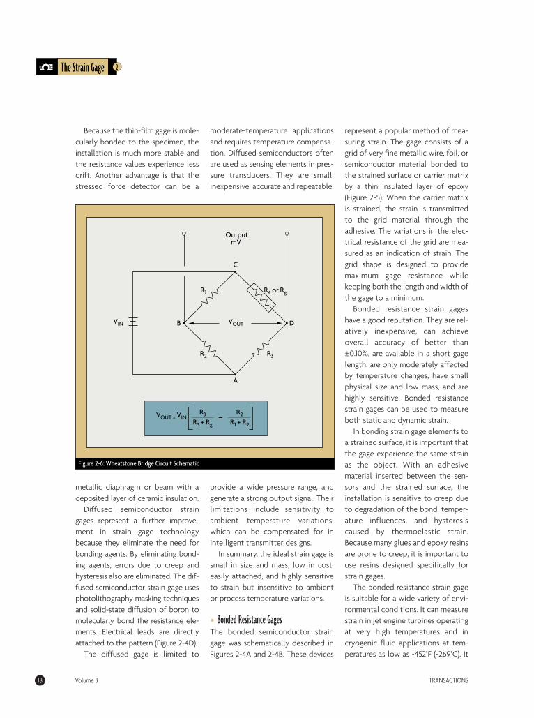
Figure 2-6: Wheatstone Bridge Circuit Schematic
VOUT
Output mV
VIN
A
C
B
R2
R1
R3
R4 or Rg
D
VOUT = VIN R3 _ R3 + Rg
R2
R1 + R2
has low mass and size, high sensitivity,and is suitable for static and dynamic
applications. Foil elements are avail-able with unit resistances from 120 to5,000 ohms. Gage lengths from0.008 in. to 4 in. are available com-mercially. The three primary consid-erations in gage selection are: oper-ating temperature, the nature of thestrain to be detected, and stabilityrequirements. In addition, selectingthe right carrier material, grid alloy,adhesive, and protective coatingwill guarantee the success of theapplication.
Measuring CircuitsIn order to measure strain with abonded resistance strain gage, itmust be connected to an electric cir-cuit that is capable of measuring theminute changes in resistance corre-sponding to strain. Strain gage trans-ducers usually employ four straingage elements electrically connect-ed to form a Wheatstone bridge cir-cuit (Figure 2-6).
A Wheatstone bridge is a dividedbridge circuit used for the measure-ment of static or dynamic electricalresistance. The output voltage of theWheatstone bridge is expressed in
millivolts output per volt input. TheWheatstone circuit is also well suited
for temperature compensation. In Figure 2-6, if R1, R2, R3, and R4 are
equal, and a voltage, VIN, is appliedbetween points A and C, then theoutput between points B and Dwill show no potential difference.
However, if R4 is changed to somevalue which does not equal R1, R2, andR3, the bridge will become unbalancedand a voltage will exist at the outputterminals. In a so-called G-bridgeconfiguration, the variable strain sen-sor has resistance Rg, while the otherarms are fixed value resistors.
The sensor, however, can occupyone, two, or four arms of the bridge,depending on the application. Thetotal strain, or output voltage of thecircuit (VOUT) is equivalent to the dif-ference between the voltage dropacross R1 and R4, or Rg. This can alsobe written as:
VOUT = VCD - VCB
For more detail, see Figure 2-6. Thebridge is considered balanced whenR1/R2 = Rg/R3 and, therefore, VOUT
equals zero.Any small change in the resis-
tance of the sensing grid will throwthe bridge out of balance, making itsuitable for the detection of strain.When the bridge is set up so that Rg
is the only active strain gage, asmall change in Rg will result in anoutput voltage from the bridge. Ifthe gage factor is GF, the strain
measurement is related to thechange in Rg as follows:
Strain = (∆Rg/Rg)/GF
The number of active strain gagesthat should be connected to thebridge depends on the application.
2 The Strain Gage
TRANSACTIONS Volume 3 19
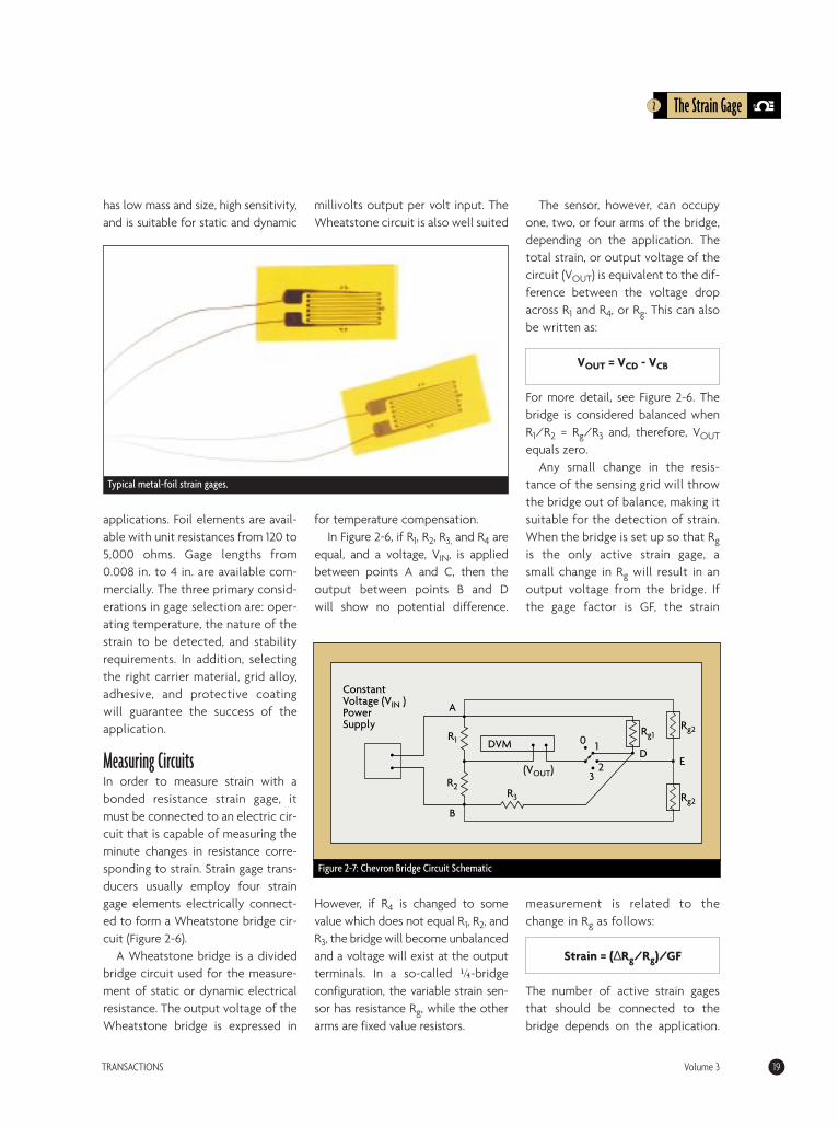
Figure 2-7: Chevron Bridge Circuit Schematic
Constant Voltage (VIN ) Power Supply
DVM
R2
Rg1 Rg2
Rg2 R3
R1
A
B
D E 3
1 0
2 (VOUT)
Typical metal-foil strain gages.
For example, it may be useful to con-nect gages that are on opposite sides
of a beam, one in compression andthe other in tension. In this arrange-ment, one can effectively double thebridge output for the same strain. Ininstallations where all of the arms areconnected to strain gages, tempera-ture compensation is automatic, asresistance change due to tempera-ture variations will be the same forall arms of the bridge.
In a four-element Wheatstonebridge, usually two gages are wired incompression and two in tension. Forexample, if R1 and R3 are in tension(positive) and R2 and R4 are in com-pression (negative), then the outputwill be proportional to the sum of allthe strains measured separately. Forgages located on adjacent legs, thebridge becomes unbalanced in pro-portion to the difference in strain. Forgages on opposite legs, the bridge bal-ances in proportion to the sum of thestrains. Whether bending strain, axialstrain, shear strain, or torsional strainis being measured, the strain gagearrangement will determine the rela-tionship between the output and thetype of strain being measured. As
shown in Figure 2-6, if a positive ten-sile strain occurs on gages R2 and R3,
and a negative strain is experienced bygages R1 and R4, the total output,VOUT, would be four times the resis-tance of a single gage.
• The Chevron BridgeThe Chevron bridge is illustrated inFigure 2-7. It is a multiple channelarrangement that serves to com-pensate for the changes in bridge-
arm resistances by periodicallyswitching them. Here, the four chan-
nel positions are used to switch thedigital voltmeter (DVM) between G-bridge (one active gage) and H-bridge (two active gages) configura-tions. The DVM measurementdevice always shares the power sup-ply and an internal H-bridge. Thisarrangement is most popular forstrain measurements on rotatingmachines, where it can reduce thenumber of slip rings required.
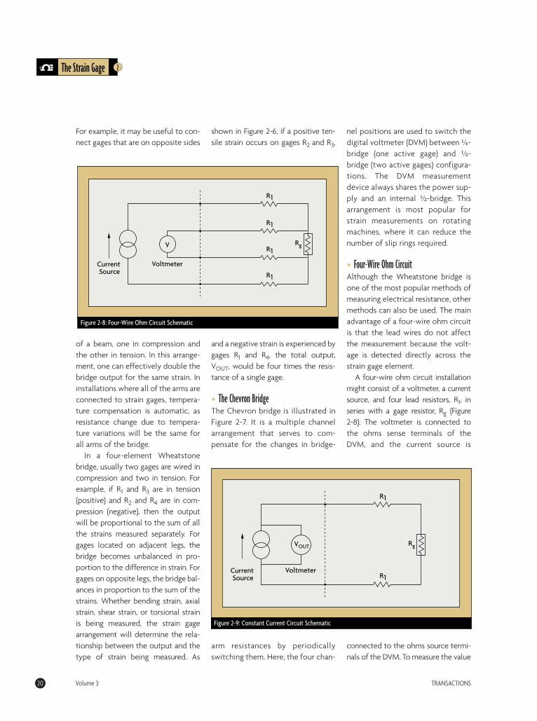
• Four-Wire Ohm CircuitAlthough the Wheatstone bridge isone of the most popular methods ofmeasuring electrical resistance, othermethods can also be used. The mainadvantage of a four-wire ohm circuitis that the lead wires do not affectthe measurement because the volt-age is detected directly across thestrain gage element.
A four-wire ohm circuit installationmight consist of a voltmeter, a currentsource, and four lead resistors, R1, inseries with a gage resistor, Rg (Figure2-8). The voltmeter is connected tothe ohms sense terminals of theDVM, and the current source is
connected to the ohms source termi-nals of the DVM. To measure the value
The Strain Gage 2
20 Volume 3 TRANSACTIONS
Figure 2-9: Constant Current Circuit Schematic
Current Source
Voltmeter
VOUT Rg
R1
R1
Figure 2-8: Four-Wire Ohm Circuit Schematic
Current Source
Voltmeter
V Rg
R1
R1
R1
R1

of strain, a low current flow (typicallyone milliampere) is supplied to thecircuit. While the voltmeter measuresthe voltage drop across Rg, theabsolute resistance value is computedby the multimeter from the values of
current and voltage.The measurement is usually done
by first measuring the value of gageresistance in an unstrained condi-tion and then making a secondmeasurement with strain applied.The difference in the measuredgage resistances divided by theunstrained resistance gives a frac-tional value of the strain. This valueis used with the gage factor (GF) tocalculate strain.
The four-wire circuit is also suitablefor automatic voltage offset compen-sation. The voltage is first measuredwhen there is no current flow. Thismeasured value is then subtractedfrom the voltage reading when cur-rent is flowing. The resulting voltage
difference is then used to computethe gage resistance. Because of theirsensitivity, four-wire strain gages aretypically used to measure low fre-quency dynamic strains. When mea-suring higher frequency strains, the
bridge output needs to be amplified.The same circuit also can be used witha semiconductor strain-gage sensorand high speed digital voltmeter. Ifthe DVM sensitivity is 100 microvolts,the current source is 0.44 mil-liamperes, the strain-gage elementresistance is 350 ohms and its gagefactor is 100, the resolution of themeasurement will be 6 microstrains.
• Constant Current CircuitResistance can be measured by excit-ing the bridge with either a constantvoltage or a constant current source.Because R = V/I, if either V or I is heldconstant, the other will vary with theresistance. Both methods can be used.
While there is no theoretical
advantage to using a constant cur-rent source (Figure 2-9) as comparedto a constant voltage, in some casesthe bridge output will be more linearin a constant current system. Also, ifa constant current source is used, iteliminates the need to sense thevoltage at the bridge; therefore, onlytwo wires need to be connected tothe strain gage element.
The constant current circuit is mosteffective when dynamic strain is beingmeasured. This is because, if a dynam-ic force is causing a change in the resis-tance of the strain gage (Rg), onewould measure the time varying com-ponent of the output (VOUT), whereasslowly changing effects such aschanges in lead resistance due to tem-perature variations would be rejected.Using this configuration, temperaturedrifts become nearly negligible.
Application & InstallationThe output of a strain gage circuit isa very low-level voltage signal requir-ing a sensitivity of 100 microvolts orbetter. The low level of the signalmakes it particularly susceptible tounwanted noise from other electricaldevices. Capacitive coupling causedby the lead wires’ running too closeto AC power cables or ground cur-rents are potential error sources instrain measurement. Other errorsources may include magneticallyinduced voltages when the leadwires pass through variable magneticfields, parasitic (unwanted) contactresistances of lead wires, insulationfailure, and thermocouple effects atthe junction of dissimilar metals. Thesum of such interferences can resultin significant signal degradation.
• ShieldingMost electric interference and noiseproblems can be solved by shielding
2 The Strain Gage
TRANSACTIONS Volume 3 21
Figure 2-10: Alternative Lead-Wire Configurations
Offset Compensated
Rg Rg DVM
i=0
4-Wire Ohms
2-Wire Bridge 3-Wire Bridge
A+
- BDVM
C
Rg DVM Rg R1
and guarding. A shield around themeasurement lead wires will inter-cept interferences and may alsoreduce any errors caused by insula-tion degradation. Shielding also willguard the measurement from capac-itive coupling. If the measurementleads are routed near electromag-netic interference sources such astransformers, twisting the leads willminimize signal degradation due tomagnetic induction. By twisting thewire, the flux-induced current is
inverted and the areas that the fluxcrosses cancel out. For industrialprocess applications, twisted andshielded lead wires are used almostwithout exception.
• GuardingGuarding the instrumentation itself isjust as important as shielding thewires. A guard is a sheet-metal boxsurrounding the analog circuitry andis connected to the shield. If groundcurrents flow through the strain-gageelement or its lead wires, aWheatstone bridge circuit cannotdistinguish them from the flow gen-erated by the current source.
Guarding guarantees that terminalsof electrical components are at thesame potential, which thereby pre-vents extraneous current flows.
Connecting a guard lead betweenthe test specimen and the negativeterminal of the power supply pro-vides an additional current patharound the measuring circuit. Byplacing a guard lead path in the pathof an error-producing current, all ofthe elements involved (i.e., floatingpower supply, strain gage, all other
measuring equipment) will be at thesame potential as the test speci-men. By using twisted and shieldedlead wires and integrating DVMswith guarding, common mode noiseerror can virtually be eliminated.
• Lead-Wire EffectsStrain gages are sometimes mountedat a distance from the measuringequipment. This increases the possi-bility of errors due to temperaturevariations, lead desensitization, andlead-wire resistance changes. In atwo-wire installation (Figure 2-10A),the two leads are in series with thestrain-gage element, and any change
in the lead-wire resistance (R1) will beindistinguishable from changes in theresistance of the strain gage (Rg).
To correct for lead-wire effects,an additional, third lead can beintroduced to the top arm of thebridge, as shown in Figure 2-10B. Inthis configuration, wire C acts as asense lead with no current flowingin it, and wires A and B are in oppo-site legs of the bridge. This is theminimum acceptable method ofwiring strain gages to a bridge tocancel at least part of the effect ofextension wire errors. Theoretically,if the lead wires to the sensor havethe same nominal resistance, thesame temperature coefficient, andare maintained at the same temper-ature, full compensation isobtained. In reality, wires are manu-factured to a tolerance of about10%, and three-wire installationdoes not completely eliminate two-wire errors, but it does reduce themby an order of magnitude. If furtherimprovement is desired, four-wireand offset-compensated installa-tions (Figures 2-10C and 2-10D)should be considered.
In two-wire installations, the errorintroduced by lead-wire resistance isa function of the resistance ratioR1/Rg. The lead error is usually not sig-nificant if the lead-wire resistance (R1)is small in comparison to the gageresistance (Rg), but if the lead-wireresistance exceeds 0.1% of the nomi-nal gage resistance, this source oferror becomes significant. Therefore,in industrial applications, lead-wirelengths should be minimized or elim-inated by locating the transmitterdirectly at the sensor.
• Temperature and the Gage FactorStrain-sensing materials, such as cop-per, change their internal structure at
The Strain Gage 2
22 Volume 3 TRANSACTIONS
Advance (Cu Ni)
Nichrome (Ni Cr)
Perc
ent
Cha
nge
In G
age
Fact
or
-400 -200 0 200 400 600 800 1000 1200 1400 1600 (-240) (-129) (-18) (93) (204) (315) (426) (538) (649) (760) (871)
120
110
100
90
80
70
Temperature °F (°C)
Karma (Ni Cr +)
Platinum- Tungsten Alloy
Figure 2-11: Gage-Factor Temperature Dependence

high temperatures. Temperature canalter not only the properties of astrain gage element, but also canalter the properties of the basematerial to which the strain gage isattached. Differences in expansioncoefficients between the gage andbase materials may cause dimension-al changes in the sensor element.
Expansion or contraction of thestrain-gage element and/or thebase material introduces errors thatare difficult to correct. For example,a change in the resistivity or in thetemperature coefficient of resis-tance of the strain gage elementchanges the zero reference used tocalibrate the unit.
The gage factor is the strain sensi-tivity of the sensor. The manufacturershould always supply data on thetemperature sensitivity of the gagefactor. Figure 2-11 shows the variationin gage factors of the various straingage materials as a function of operat-ing temperature. Copper-nickel alloyssuch as Advance have gage factorsthat are relatively sensitive to operat-ing temperature variations, makingthem the most popular choice forstrain gage materials.
• Apparent StrainApparent strain is any change in gageresistance that is not caused by thestrain on the force element.Apparent strain is the result of theinteraction of the thermal coeffi-cient of the strain gage and the dif-ference in expansion between thegage and the test specimen. The vari-ation in the apparent strain of vari-ous strain-gage materials as a func-tion of operating temperature isshown in Figure 2-12. In addition tothe temperature effects, apparentstrain also can change because ofaging and instability of the metal and
the bonding agent.Compensation for apparent
strain is necessary if the tempera-ture varies while the strain is beingmeasured. In most applications, theamount of error depends on thealloy used, the accuracy required,and the amount of the temperaturevariation. If the operating tempera-ture of the gage and the apparentstrain characteristics are known,compensation is possible.
• Stability ConsiderationsIt is desirable that the strain-gagemeasurement system be stable andnot drift with time. In calibratedinstruments, the passage of time
always causes some drift and loss ofcalibration. The stability of bondedstrain-gage transducers is inferior tothat of diffused strain-gage ele-ments. Hysteresis and creepingcaused by imperfect bonding is oneof the fundamental causes of insta-
bility, particularly in high operatingtemperature environments.
Before mounting strain-gage ele-ments, it should be established thatthe stressed force detector itself isuniform and homogeneous, becauseany surface deformities will result ininstability errors. In order to removeany residual stresses in the forcedetectors, they should be carefullyannealed, hardened, and stress-relieved using temperature aging. Atransducer that uses force-detectorsprings, diaphragms, or bellowsshould also be provided withmechanical isolation. This will pro-tect the sensor element from exter-nal stresses caused either by the
strain of mounting or by the attachingof electric conduits to the transducer.
If stable sensors are used, such asdeposited thin-film element types,and if the force-detector structure iswell designed, balancing and com-pensation resistors will be sufficient
2 The Strain Gage
TRANSACTIONS Volume 3 23
Apparent Strain Slope 10-6 Inches/Inch/°F (Microns/mm/°C)
Platinum Tungsten Alloy
Nichrome
Karma
Advance
Base Reference Stainless Steel
500 600 700 800 900 1000 1100 1200 1300(260) (315) (371) (426) (482) (538) (593) (649) (704)
100
75
50
20
10
0
-5
(0.180)
(0.135)
(0.090)
(0.036)
(0.018)
(-0.009)
Temperature °F (°C)
Figure 2-12: Apparent Strain Variation with Temperature
for periodic recalibration of the unit.The most stable sensors are madefrom platinum or other low-temper-ature coefficient materials. It is alsoimportant that the transducer beoperated within its design limits.
Otherwise, permanent calibrationshifts can result. Exposing the trans-ducer to temperatures outside itsoperating limits can also degradeperformance. Similarly, the transduc-er should be protected from vibra-tion, acceleration, and shock.
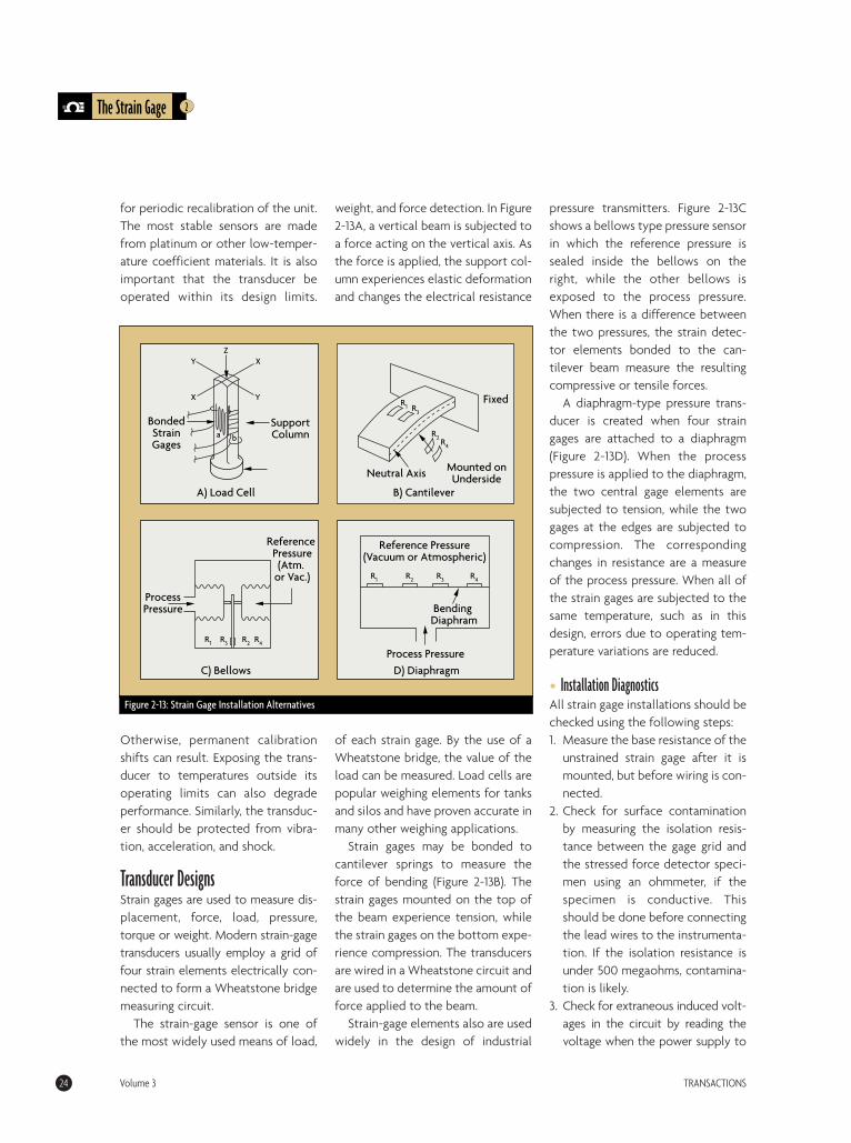
Transducer DesignsStrain gages are used to measure dis-placement, force, load, pressure,torque or weight. Modern strain-gagetransducers usually employ a grid offour strain elements electrically con-nected to form a Wheatstone bridgemeasuring circuit.
The strain-gage sensor is one ofthe most widely used means of load,
weight, and force detection. In Figure2-13A, a vertical beam is subjected toa force acting on the vertical axis. Asthe force is applied, the support col-umn experiences elastic deformationand changes the electrical resistance
of each strain gage. By the use of aWheatstone bridge, the value of theload can be measured. Load cells arepopular weighing elements for tanksand silos and have proven accurate inmany other weighing applications.
Strain gages may be bonded tocantilever springs to measure theforce of bending (Figure 2-13B). Thestrain gages mounted on the top ofthe beam experience tension, whilethe strain gages on the bottom expe-rience compression. The transducersare wired in a Wheatstone circuit andare used to determine the amount offorce applied to the beam.
Strain-gage elements also are usedwidely in the design of industrial
pressure transmitters. Figure 2-13Cshows a bellows type pressure sensorin which the reference pressure issealed inside the bellows on theright, while the other bellows isexposed to the process pressure.When there is a difference betweenthe two pressures, the strain detec-tor elements bonded to the can-tilever beam measure the resultingcompressive or tensile forces.
A diaphragm-type pressure trans-ducer is created when four straingages are attached to a diaphragm(Figure 2-13D). When the processpressure is applied to the diaphragm,the two central gage elements aresubjected to tension, while the twogages at the edges are subjected tocompression. The correspondingchanges in resistance are a measureof the process pressure. When all ofthe strain gages are subjected to thesame temperature, such as in thisdesign, errors due to operating tem-perature variations are reduced.
• Installation DiagnosticsAll strain gage installations should bechecked using the following steps:1. Measure the base resistance of the
unstrained strain gage after it ismounted, but before wiring is con-nected.
2. Check for surface contaminationby measuring the isolation resis-tance between the gage grid andthe stressed force detector speci-men using an ohmmeter, if thespecimen is conductive. Thisshould be done before connectingthe lead wires to the instrumenta-tion. If the isolation resistance isunder 500 megaohms, contamina-tion is likely.
3. Check for extraneous induced volt-ages in the circuit by reading thevoltage when the power supply to
The Strain Gage 2
24 Volume 3 TRANSACTIONS
Figure 2-13: Strain Gage Installation Alternatives
D) Diaphragm
R1 R2 R3 R4
Reference Pressure (Vacuum or Atmospheric)
Z
Bending Diaphram
Process Pressure
Reference Pressure (Atm.
or Vac.)
Process Pressure
C) Bellows
R1 R3 R2 R4
R1 R3
R2R4
Mounted on Underside
Fixed
Neutral Axis
B) Cantilever
Support Column
Bonded Strain Gages
a b
XZ
X
Y
Y
A) Load Cell

the bridge is disconnected. Bridgeoutput voltage readings for eachstrain-gage channel should benearly zero.
4. Connect the excitation powersupply to the bridge and ensureboth the correct voltage level andits stability.
5. Check the strain gage bond byapplying pressure to the gage. Thereading should be unaffected. T
2 The Strain Gage
TRANSACTIONS Volume 3 25
References & Further Reading• Omegadyne®Pressure, Force, Load, Torque Databook, OMEGADYNE, Inc.,
1996.• The Pressure, Strain, and Force Handbook™, Omega Press LLC, 1996.• Instrument Engineers’ Handbook, Bela Liptak, CRC Press LLC, 1995. • Marks’ Standard Handbook for Mechanical Engineers, 10th Edition,
Eugene A. Avallone and Theodore Baumeister, McGraw-Hill, 1996.• McGraw-Hill Concise Encyclopedia of Science and Technology, McGraw-
Hill, 1998.• Process/Industrial Instruments and Controls Handbook, 4th Edition,
Douglas M. Considine, McGraw-Hill, 1993.• Van Nostrand’s Scientific Encyclopedia, Douglas M. Considine and Glenn
D. Considine, Van Nostrand, 1997.
Mechanical methods ofmeasuring pressure havebeen known for centuries.U-tube manometers were
among the first pressure indicators.Originally, these tubes were made ofglass, and scales were added to themas needed. But manometers are large,cumbersome, and not well suited forintegration into automatic controlloops. Therefore, manometers areusually found in the laboratory orused as local indicators. Dependingon the reference pressure used, theycould indicate absolute, gauge, anddifferential pressure.
Differential pressure transducersoften are used in flow measurementwhere they can measure the pressuredifferential across a venturi, orifice, orother type of primary element. Thedetected pressure differential is relat-ed to flowing velocity and thereforeto volumetric flow. Many features ofmodern pressure transmitters havecome from the differential pressuretransducer. In fact, one might consider
the differential pressure transmitterthe model for all pressure transducers.
“Gauge” pressure is defined relativeto atmospheric conditions. In thoseparts of the world that continue touse English units, gauge pressure isindicated by adding a “g” to the unitsdescriptor. Therefore, the pressureunit “pounds per square inch gauge” isabbreviated psig. When using SI units,it is proper to add “gauge” to the unitsused, such as “Pa gauge.” When pres-sure is to be measured in absoluteunits, the reference is full vacuum andthe abbreviation for “pounds persquare inch absolute” is psia.
Often, the terms pressure gauge,sensor, transducer, and transmitterare used interchangeably. The termpressure gauge usually refers to aself-contained indicator that con-verts the detected process pressureinto the mechanical motion of apointer. A pressure transducer mightcombine the sensor element of agauge with a mechanical-to-electri-cal or mechanical-to-pneumatic con-
verter and a power supply. A pressuretransmitter is a standardized pressuremeasurement package consisting ofthree basic components: a pressuretransducer, its power supply, and asignal conditioner/retransmitter thatconverts the transducer signal into astandardized output.
Pressure transmitters can sendthe process pressure of interestusing an analog pneumatic (3-15psig), analog electronic (4-20 mAdc), or digital electronic signal.When transducers are directly inter-faced with digital data acquisitionsystems and are located at some
distance from the data acquisitionhardware, high output voltage sig-nals are preferred. These signalsmust be protected against both elec-tromagnetic and radio frequencyinterference (EMI/RFI) when travel-ing longer distances.
Pressure transducer performance-related terms also require definition.Transducer accuracy refers to thedegree of conformity of the mea-
26 Volume 3 TRANSACTIONS
From Mechanical to Electronic
Transducer Types
Practical Considerations
FORCE-RELATED MEASUREMENTSProcess Pressure Measurement
3
MProcess Pressure Measurement
Figure 3-1: Bourdon Tube Designs
Moving Tip
Process Pressure
Process Pressure
µ
A
A
Process Pressure
C-Bourdon Spiral Helical
sured value to an accepted standard.It is usually expressed as a percent-age of either the full scale or of theactual reading of the instrument. In
case of percent-full-scale devices,error increases as the absolute valueof the measurement drops.Repeatability refers to the closenessof agreement among a number ofconsecutive measurements of thesame variable. Linearity is a measureof how well the transducer outputincreases linearly with increasingpressure. Hysteresis error describesthe phenomenon whereby the sameprocess pressure results in differentoutput signals depending uponwhether the pressure is approachedfrom a lower or higher pressure.
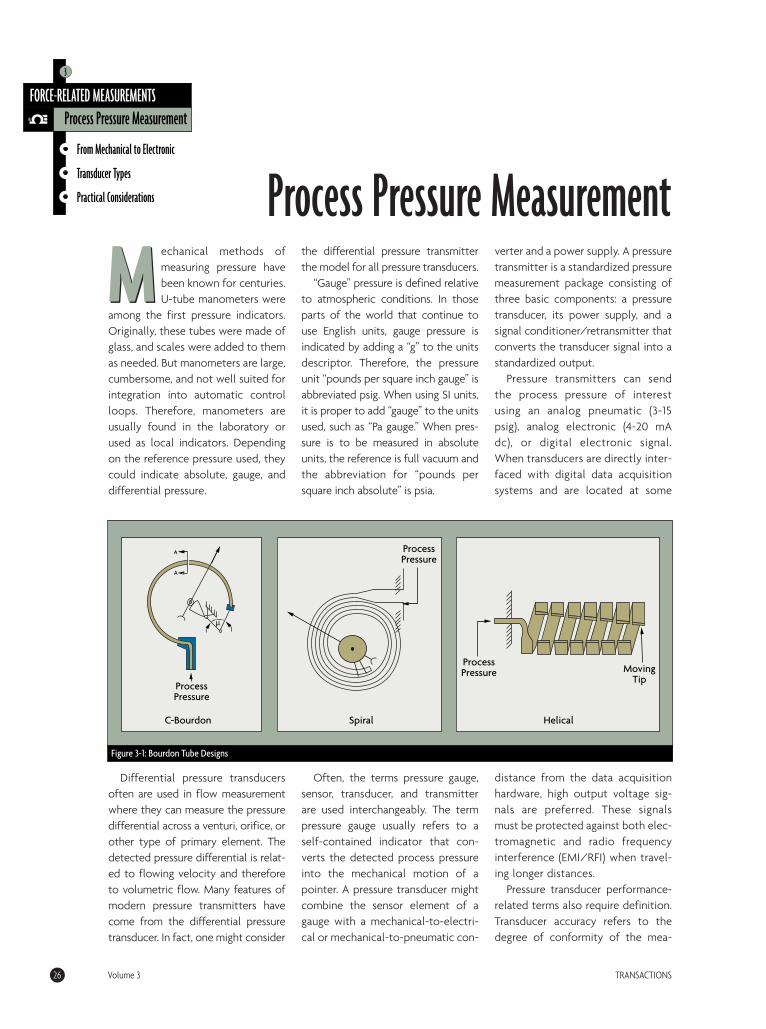
From Mechanical to ElectronicThe first pressure gauges used flexi-ble elements as sensors. As pressurechanged, the flexible element
moved, and this motion was used torotate a pointer in front of a dial. Inthese mechanical pressure sensors,a Bourdon tube, a diaphragm, or abellows element detected theprocess pressure and caused a cor-responding movement.
A Bourdon tube is C-shaped andhas an oval cross-section with oneend of the tube connected to theprocess pressure (Figure 3-1A). Theother end is sealed and connected tothe pointer or transmitter mecha-nism. To increase their sensitivity,Bourdon tube elements can be
extended into spirals or helical coils(Figures 3-1B and 3-1C). This increasestheir effective angular length andtherefore increases the movement at
their tip, which in turn increases theresolution of the transducer.
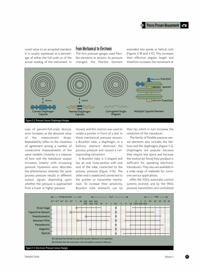
The family of flexible pressure sen-sor elements also includes the bel-lows and the diaphragms (Figure 3-2).Diaphragms are popular becausethey require less space and becausethe motion (or force) they produce issufficient for operating electronictransducers. They also are available ina wide range of materials for corro-sive service applications.
After the 1920s, automatic controlsystems evolved, and by the 1950spressure transmitters and centralized
3 Process Pressure Measurement
TRANSACTIONS Volume 3 27
Convex Diaphragm Capsule
Motion
Nested Diaphragm Capsule
Motion
Corrugated Single Diagram
Multiple Capsule Element
Free End
Spacers
Fixed End
Figure 3-2: Pressure Sensor Diaphragm Designs
Figure 3-3: Electronic Pressure Sensor Ranges
Strain Gage
Capacitive Sensors
Potentiometric
Resonant Wire
Piezoelectric
Magnetic
Optical
10-14 10-10 10-6 10-3 10-1 1 50 200 400 600 4 7 11 102 103 104 105 106
-300 -200 -100 -10 -5 -1 0.1 +1 +5 +10 +100 +200 +300+-
V
V
V
V
V
A
A
A
A
A
A
A
mmHg absolute
V Indicates that the device uses full-vacuum reference in its operation
A Indicates that the instrument uses atmospheric pressure reference
"H20 PSIG
control rooms were commonplace.Therefore, the free end of a Bourdontube (bellows or diaphragm) nolonger had to be connected to alocal pointer, but served to convert aprocess pressure into a transmitted(electrical or pneumatic) signal. Atfirst, the mechanical linkage was con-nected to a pneumatic pressuretransmitter, which usually generateda 3-15 psig output signal for transmis-sion over distances of several hun-dred feet, or even farther withbooster repeaters. Later, as solidstate electronics matured and trans-mission distances increased, pressuretransmitters became electronic. Theearly designs generated dc voltageoutputs (10-50 mV; 1-5 V; 0-100 mV),but later were standardized as 4-20mA dc current output signals.
Because of the inherent limita-tions of mechanical motion-balancedevices, first the force-balance andlater the solid state pressure transduc-er were introduced. The first unbond-ed-wire strain gages were introducedin the late 1930s. In this device, thewire filament is attached to a struc-ture under strain, and the resistance in
the strained wire is measured. Thisdesign was inherently unstable andcould not maintain calibration. There
also were problems with degradationof the bond between the wire fila-ment and the diaphragm, and withhysteresis caused by thermoelasticstrain in the wire.
The search for improved pressureand strain sensors first resulted in theintroduction of bonded thin-film andfinally diffused semiconductor straingages. These were first developed forthe automotive industry, but shortlythereafter moved into the generalfield of pressure measurement andtransmission in all industrial and sci-entific applications. Semiconductorpressure sensors are sensitive, inex-pensive, accurate and repeatable.(For more details on strain gage oper-ation, see Chapter 2.)
Many pneumatic pressure trans-mitters are still in operation, particu-
3Process Pressure Measurement
28 Volume 3 TRANSACTIONS
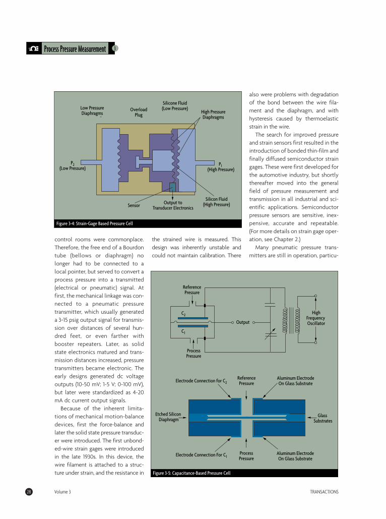
Figure 3-4: Strain-Gage Based Pressure Cell
Low Pressure Diaphragms
Overload Plug
Silicone Fluid (Low Pressure)
High Pressure Diaphragms
P2 (Low Pressure)
Output to Transducer ElectronicsSensor
Silicon Fluid (High Pressure)
P1 (High Pressure)
High Frequency Oscillator
C2
C1
Output
Reference Pressure
Process Pressure
Electrode Connection for C2Reference Pressure
Aluminum Electrode On Glass Substrate
Glass Substrates
Aluminum Electrode On Glass Substrate
Electrode Connection For C1Process Pressure
Etched Silicon Diaphragm
Figure 3-5: Capacitance-Based Pressure Cell
larly in the petrochemical industry.But as control systems continue tobecome more centralized and com-puterized, these devices have beenreplaced by analog electronic and,more recently, digital electronictransmitters.
Transducer TypesFigure 3-3 provides an overall orienta-tion to the scientist or engineer whomight be faced with the task of select-ing a pressure detector from amongthe many designs available. This tableshows the ranges of pressures and vac-uums that various sensor types arecapable of detecting and the types ofinternal references (vacuum or atmos-pheric pressure) used, if any.
Because electronic pressure trans-ducers are of greatest utility forindustrial and laboratory data acqui-sition and control applications, theoperating principles and pros andcons of each of these is further elab-orated in this section.
• Strain GageWhen a strain gage, as described indetail in Chapter 2, is used to mea-
sure the deflection of an elasticdiaphragm or Bourdon tube, itbecomes a component in a pressuretransducer. Strain gage-type pressure
transducers are widely used. Strain-gage transducers are used
for narrow-span pressure and fordifferential pressure measurements.Essentially, the strain gage is usedto measure the displacement of anelastic diaphragm due to a differ-ence in pressure across the
diaphragm. These devices candetect gauge pressure if the lowpressure port is left open to theatmosphere or differential pressure
if connected to two process pres-sures. If the low pressure side is asealed vacuum reference, the trans-mitter will act as an absolute pres-sure transmitter.
Strain gage transducers are avail-able for pressure ranges as low as3 inches of water to as high as200,000 psig (1400 MPa). Inaccuracyranges from 0.1% of span to 0.25% offull scale. Additional error sourcescan be a 0.25% of full scale drift oversix months and a 0.25% full scaletemperature effect per 1000° F.
• CapacitanceCapacitance pressure transducerswere originally developed for use inlow vacuum research. This capaci-tance change results from themovement of a diaphragm element(Figure 3-5). The diaphragm is usuallymetal or metal-coated quartz and isexposed to the process pressure onone side and to the reference pressureon the other. Depending on the type
3 Process Pressure Measurement
TRANSACTIONS Volume 3 29
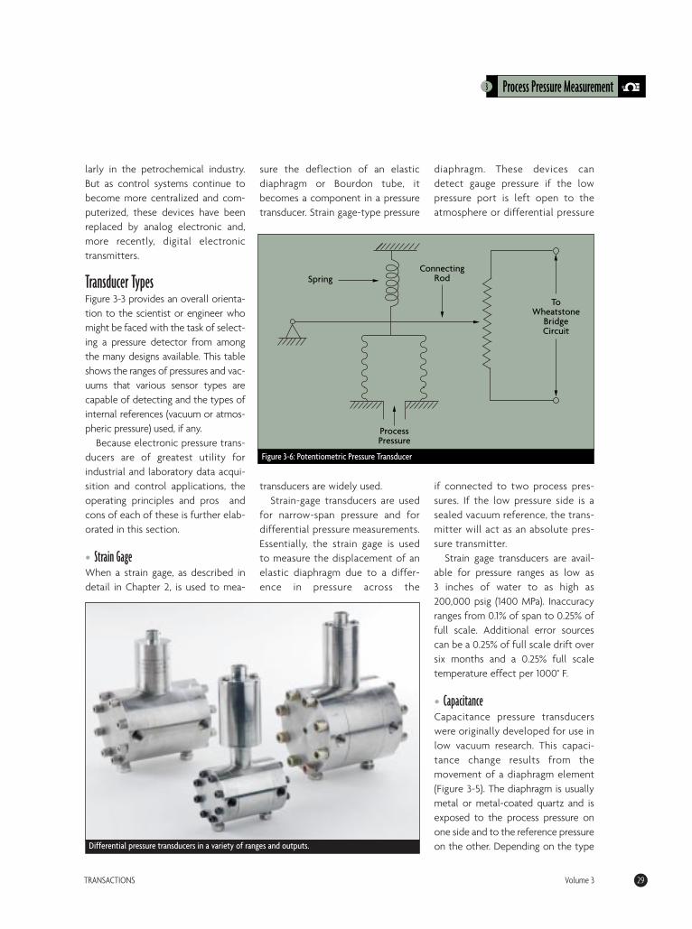
Connecting Rod
Process Pressure
To Wheatstone
Bridge Circuit
Spring
Figure 3-6: Potentiometric Pressure Transducer
Differential pressure transducers in a variety of ranges and outputs.
of pressure, the capacitive transducercan be either an absolute, gauge, ordifferential pressure transducer.
Stainless steel is the most commondiaphragm material used, but for cor-rosive service, high-nickel steel alloys,
such as Inconel or Hastelloy, give bet-ter performance. Tantalum also isused for highly corrosive, high tem-perature applications. As a specialcase, silver diaphragms can be usedto measure the pressure of chlorine,fluorine, and other halogens in theirelemental state.
In a capacitance-type pressure sen-sor, a high-frequency, high-voltageoscillator is used to charge the sensingelectrode elements. In a two-platecapacitor sensor design, the move-ment of the diaphragm between the
plates is detected as an indication ofthe changes in process pressure.
As shown in Figure 3-5, the deflec-tion of the diaphragm causes achange in capacitance that is detect-ed by a bridge circuit. This circuit can
be operated in either a balanced orunbalanced mode. In balanced mode,the output voltage is fed to a nulldetector and the capacitor arms arevaried to maintain the bridge at null.Therefore, in the balanced mode, thenull setting itself is a measure ofprocess pressure. When operated inunbalanced mode, the process pres-sure measurement is related to theratio between the output voltageand the excitation voltage.
Single-plate capacitor designs arealso common. In this design, the
plate is located on the back side ofthe diaphragm and the variablecapacitance is a function of deflec-tion of the diaphragm. Therefore,the detected capacitance is an indi-cation of the process pressure. Thecapacitance is converted into eithera direct current or a voltage signalthat can be read directly by panelmeters or microprocessor-basedinput/output boards.
Capacitance pressure transducersare widespread in part because oftheir wide rangeability, from high vac-uums in the micron range to 10,000psig (70 MPa). Differential pressures aslow as 0.01 inches of water can readi-ly be measured. And, compared withstrain gage transducers, they do notdrift much. Better designs are avail-able that are accurate to within 0.1%of reading or 0.01% of full scale. Atypical temperature effect is 0.25% offull scale per 1000° F.
Capacitance-type sensors areoften used as secondary standards,especially in low-differential andlow-absolute pressure applications.They also are quite responsive,because the distance the diaphragmmust physically travel is only a fewmicrons. Newer capacitance pressuretransducers are more resistant tocorrosion and are less sensitive tostray capacitance and vibrationeffects that used to cause “readingjitters” in older designs.
• PotentiometricThe potentiometric pressure sensorprovides a simple method for obtain-ing an electronic output from amechanical pressure gauge. Thedevice consists of a precision poten-tiometer, whose wiper arm is mechan-ically linked to a Bourdon or bellowselement. The movement of thewiper arm across the potentiometer
3Process Pressure Measurement
30 Volume 3 TRANSACTIONS
Electromagnetic Plucking and Sensing Coil
Wire Grip
Vibrating Wire
Wire Grip
Pressure-Sensitive Diaphragm
Resonant WireTo Oscillator
Circuit
High-Side Backup Plate
Metal Tube
High-Pressure Diaphragm
Fluid Transfer Port
Low-Pressure Diaphragm
Electrical Insulator
Preload Spring
Low-Side Backup Plate
Magnet
Magnet
Figure 3-7: Resonant-Wire Pressure Transducer
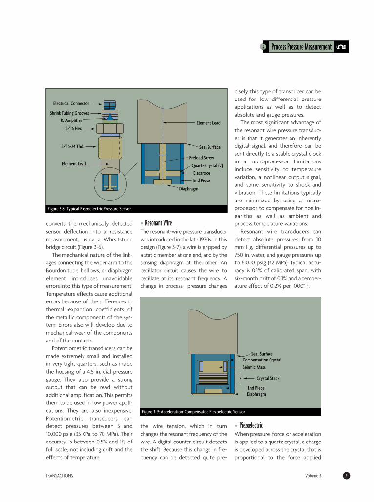
converts the mechanically detectedsensor deflection into a resistancemeasurement, using a Wheatstonebridge circuit (Figure 3-6).
The mechanical nature of the link-ages connecting the wiper arm to theBourdon tube, bellows, or diaphragmelement introduces unavoidableerrors into this type of measurement.Temperature effects cause additionalerrors because of the differences inthermal expansion coefficients ofthe metallic components of the sys-tem. Errors also will develop due tomechanical wear of the componentsand of the contacts.
Potentiometric transducers can bemade extremely small and installedin very tight quarters, such as insidethe housing of a 4.5-in. dial pressuregauge. They also provide a strongoutput that can be read withoutadditional amplification. This permitsthem to be used in low power appli-cations. They are also inexpensive.Potentiometric transducers candetect pressures between 5 and10,000 psig (35 KPa to 70 MPa). Theiraccuracy is between 0.5% and 1% offull scale, not including drift and theeffects of temperature.
• Resonant WireThe resonant-wire pressure transducerwas introduced in the late 1970s. In thisdesign (Figure 3-7), a wire is gripped bya static member at one end, and by thesensing diaphragm at the other. Anoscillator circuit causes the wire tooscillate at its resonant frequency. Achange in process pressure changes
the wire tension, which in turnchanges the resonant frequency of thewire. A digital counter circuit detectsthe shift. Because this change in fre-quency can be detected quite pre-
cisely, this type of transducer can beused for low differential pressureapplications as well as to detectabsolute and gauge pressures.
The most significant advantage ofthe resonant wire pressure transduc-er is that it generates an inherentlydigital signal, and therefore can besent directly to a stable crystal clockin a microprocessor. Limitationsinclude sensitivity to temperaturevariation, a nonlinear output signal,and some sensitivity to shock andvibration. These limitations typicallyare minimized by using a micro-processor to compensate for nonlin-earities as well as ambient andprocess temperature variations.
Resonant wire transducers candetect absolute pressures from 10mm Hg, differential pressures up to750 in. water, and gauge pressures upto 6,000 psig (42 MPa). Typical accu-racy is 0.1% of calibrated span, withsix-month drift of 0.1% and a temper-ature effect of 0.2% per 1000° F.
• PiezoelectricWhen pressure, force or accelerationis applied to a quartz crystal, a chargeis developed across the crystal that isproportional to the force applied
3 Process Pressure Measurement
TRANSACTIONS Volume 3 31
Element Lead
Seal Surface
Preload Screw
Quartz Crystal (2)
Electrode
End Piece
Diaphragm
Electrical Connector
Shrink Tubing Grooves
IC Amplifier
5/16 Hex
5/16-24 Thd.
Element Lead
Figure 3-8: Typical Piezoelectric Pressure Sensor
Seal SurfaceCompensation Crystal
Seismic Mass
Crystal Stack
End PieceDiaphragm
Figure 3-9: Acceleration-Compensated Piezoelectric Sensor
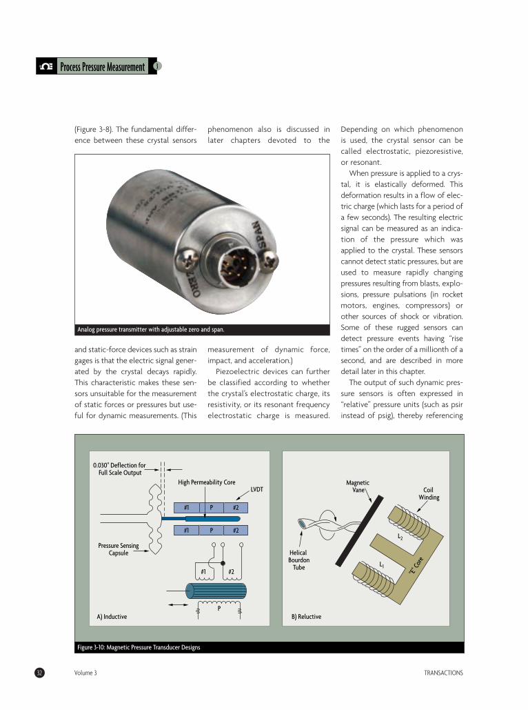
(Figure 3-8). The fundamental differ-ence between these crystal sensors
and static-force devices such as straingages is that the electric signal gener-ated by the crystal decays rapidly.This characteristic makes these sen-sors unsuitable for the measurementof static forces or pressures but use-ful for dynamic measurements. (This
phenomenon also is discussed inlater chapters devoted to the
measurement of dynamic force,impact, and acceleration.)
Piezoelectric devices can furtherbe classified according to whetherthe crystal’s electrostatic charge, itsresistivity, or its resonant frequencyelectrostatic charge is measured.
Depending on which phenomenonis used, the crystal sensor can becalled electrostatic, piezoresistive,or resonant.
When pressure is applied to a crys-tal, it is elastically deformed. Thisdeformation results in a flow of elec-tric charge (which lasts for a period ofa few seconds). The resulting electricsignal can be measured as an indica-tion of the pressure which wasapplied to the crystal. These sensorscannot detect static pressures, but areused to measure rapidly changingpressures resulting from blasts, explo-sions, pressure pulsations (in rocketmotors, engines, compressors) orother sources of shock or vibration.Some of these rugged sensors candetect pressure events having “risetimes” on the order of a millionth of asecond, and are described in moredetail later in this chapter.
The output of such dynamic pres-sure sensors is often expressed in“relative” pressure units (such as psirinstead of psig), thereby referencing
3Process Pressure Measurement
32 Volume 3 TRANSACTIONS
B) Reluctive
Coil Winding
"E" Co
re
L2
L1
#1
#1
P
P
#2
#2
0.030" Deflection for Full Scale Output
High Permeability Core
Pressure Sensing Capsule
LVDT
#1 #2
P
Helical Bourdon
Tube
Magnetic Vane
A) Inductive
Figure 3-10: Magnetic Pressure Transducer Designs
Analog pressure transmitter with adjustable zero and span.
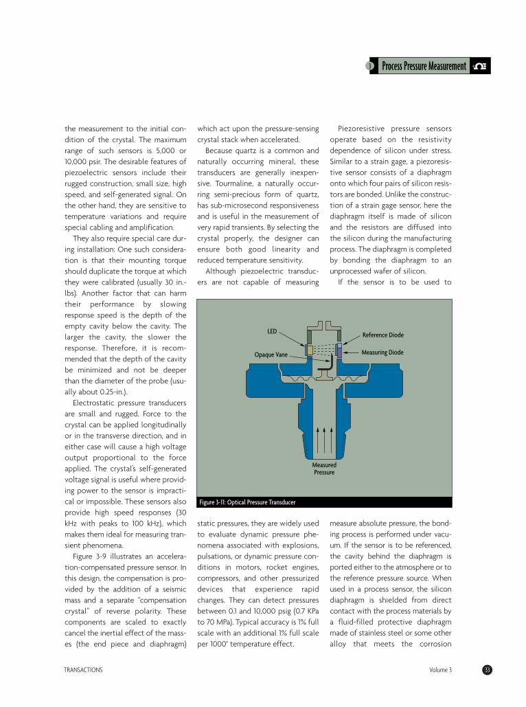
the measurement to the initial con-dition of the crystal. The maximumrange of such sensors is 5,000 or10,000 psir. The desirable features ofpiezoelectric sensors include theirrugged construction, small size, highspeed, and self-generated signal. Onthe other hand, they are sensitive totemperature variations and requirespecial cabling and amplification.
They also require special care dur-ing installation: One such considera-tion is that their mounting torqueshould duplicate the torque at whichthey were calibrated (usually 30 in.-lbs). Another factor that can harmtheir performance by slowingresponse speed is the depth of theempty cavity below the cavity. Thelarger the cavity, the slower theresponse. Therefore, it is recom-mended that the depth of the cavitybe minimized and not be deeperthan the diameter of the probe (usu-ally about 0.25-in.).
Electrostatic pressure transducersare small and rugged. Force to thecrystal can be applied longitudinallyor in the transverse direction, and ineither case will cause a high voltageoutput proportional to the forceapplied. The crystal’s self-generatedvoltage signal is useful where provid-ing power to the sensor is impracti-cal or impossible. These sensors alsoprovide high speed responses (30kHz with peaks to 100 kHz), whichmakes them ideal for measuring tran-sient phenomena.
Figure 3-9 illustrates an accelera-tion-compensated pressure sensor. Inthis design, the compensation is pro-vided by the addition of a seismicmass and a separate “compensationcrystal” of reverse polarity. Thesecomponents are scaled to exactlycancel the inertial effect of the mass-es (the end piece and diaphragm)
which act upon the pressure-sensingcrystal stack when accelerated.
Because quartz is a common andnaturally occurring mineral, thesetransducers are generally inexpen-sive. Tourmaline, a naturally occur-ring semi-precious form of quartz,has sub-microsecond responsivenessand is useful in the measurement ofvery rapid transients. By selecting thecrystal properly, the designer canensure both good linearity andreduced temperature sensitivity.
Although piezoelectric transduc-ers are not capable of measuring
static pressures, they are widely usedto evaluate dynamic pressure phe-nomena associated with explosions,pulsations, or dynamic pressure con-ditions in motors, rocket engines,compressors, and other pressurizeddevices that experience rapidchanges. They can detect pressuresbetween 0.1 and 10,000 psig (0.7 KPato 70 MPa). Typical accuracy is 1% fullscale with an additional 1% full scaleper 1000° temperature effect.
Piezoresistive pressure sensorsoperate based on the resistivitydependence of silicon under stress.Similar to a strain gage, a piezoresis-tive sensor consists of a diaphragmonto which four pairs of silicon resis-tors are bonded. Unlike the construc-tion of a strain gage sensor, here thediaphragm itself is made of siliconand the resistors are diffused intothe silicon during the manufacturingprocess. The diaphragm is completedby bonding the diaphragm to anunprocessed wafer of silicon.
If the sensor is to be used to
measure absolute pressure, the bond-ing process is performed under vacu-um. If the sensor is to be referenced,the cavity behind the diaphragm isported either to the atmosphere or tothe reference pressure source. Whenused in a process sensor, the silicondiaphragm is shielded from directcontact with the process materials bya fluid-filled protective diaphragmmade of stainless steel or some otheralloy that meets the corrosion
3 Process Pressure Measurement
TRANSACTIONS Volume 3 33
Figure 3-11: Optical Pressure Transducer
Measured Pressure
Measuring Diode
Reference DiodeLED
Opaque Vane
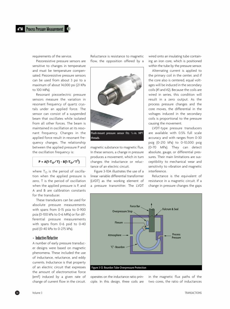
requirements of the service.Piezoresistive pressure sensors are
sensitive to changes in temperatureand must be temperature compen-sated. Piezoresistive pressure sensorscan be used from about 3 psi to amaximum of about 14,000 psi (21 KPato 100 MPa).
Resonant piezoelectric pressuresensors measure the variation inresonant frequency of quartz crys-tals under an applied force. Thesensor can consist of a suspendedbeam that oscillates while isolatedfrom all other forces. The beam ismaintained in oscillation at its reso-nant frequency. Changes in theapplied force result in resonant fre-quency changes. The relationshipbetween the applied pressure P andthe oscillation frequency is:
P = A(1-TO/T) - B(1-TO/T2)
where TO is the period of oscilla-tion when the applied pressure iszero, T is the period of oscillationwhen the applied pressure is P, andA and B are calibration constantsfor the transducer.
These transducers can be used forabsolute pressure measurementswith spans from 0-15 psia to 0-900psia (0-100 kPa to 0-6 MPa) or for dif-ferential pressure measurementswith spans from 0-6 psid to 0-40psid (0-40 kPa to 0-275 kPa).
• Inductive/ReluctiveA number of early pressure transduc-er designs were based on magneticphenomena. These included the useof inductance, reluctance, and eddycurrents. Inductance is that propertyof an electric circuit that expressesthe amount of electromotive force(emf) induced by a given rate ofchange of current flow in the circuit.
Reluctance is resistance to magneticflow, the opposition offered by a
magnetic substance to magnetic flux.In these sensors, a change in pressureproduces a movement, which in turnchanges the inductance or reluc-tance of an electric circuit.
Figure 3-10A illustrates the use of alinear variable differential transformer(LVDT) as the working element ofa pressure transmitter. The LVDT
operates on the inductance ratio prin-ciple. In this design, three coils are
wired onto an insulating tube contain-ing an iron core, which is positionedwithin the tube by the pressure sensor.
Alternating current is applied tothe primary coil in the center, and ifthe core also is centered, equal volt-ages will be induced in the secondarycoils (#1 and #2). Because the coils arewired in series, this condition willresult in a zero output. As theprocess pressure changes and thecore moves, the differential in thevoltages induced in the secondarycoils is proportional to the pressurecausing the movement.
LVDT-type pressure transducersare available with 0.5% full scaleaccuracy and with ranges from 0-30psig (0-210 kPa) to 0-10,000 psig(0-70 MPa). They can detectabsolute, gauge, or differential pres-sures. Their main limitations are sus-ceptibility to mechanical wear andsensitivity to vibration and magneticinterference.
Reluctance is the equivalent ofresistance in a magnetic circuit. If achange in pressure changes the gaps
in the magnetic flux paths of thetwo cores, the ratio of inductances
3Process Pressure Measurement
34 Volume 3 TRANSACTIONS
Force Bar
Overpressure Stop
Flexure
Atmosphere
"C"- Bourdon
Fulcrum & Seal
Process Pressure
Figure 3-12: Bourdon Tube Overpressure Protection
Flush-mount pressure sensor fits G-in. NPT
threads.
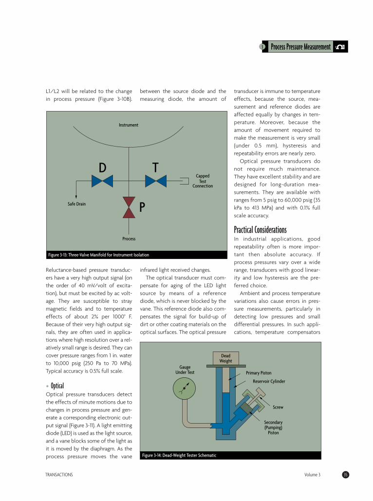
L1/L2 will be related to the changein process pressure (Figure 3-10B).
Reluctance-based pressure transduc-ers have a very high output signal (onthe order of 40 mV/volt of excita-tion), but must be excited by ac volt-age. They are susceptible to straymagnetic fields and to temperatureeffects of about 2% per 1000° F.Because of their very high output sig-nals, they are often used in applica-tions where high resolution over a rel-atively small range is desired. They cancover pressure ranges from 1 in. waterto 10,000 psig (250 Pa to 70 MPa).Typical accuracy is 0.5% full scale.
• OpticalOptical pressure transducers detectthe effects of minute motions due tochanges in process pressure and gen-erate a corresponding electronic out-put signal (Figure 3-11). A light emittingdiode (LED) is used as the light source,and a vane blocks some of the light asit is moved by the diaphragm. As theprocess pressure moves the vane
between the source diode and themeasuring diode, the amount of
infrared light received changes.The optical transducer must com-
pensate for aging of the LED lightsource by means of a referencediode, which is never blocked by thevane. This reference diode also com-pensates the signal for build-up ofdirt or other coating materials on theoptical surfaces. The optical pressure
transducer is immune to temperatureeffects, because the source, mea-surement and reference diodes areaffected equally by changes in tem-perature. Moreover, because theamount of movement required tomake the measurement is very small(under 0.5 mm), hysteresis andrepeatability errors are nearly zero.
Optical pressure transducers donot require much maintenance.They have excellent stability and aredesigned for long-duration mea-surements. They are available withranges from 5 psig to 60,000 psig (35kPa to 413 MPa) and with 0.1% fullscale accuracy.
Practical ConsiderationsIn industrial applications, goodrepeatability often is more impor-tant then absolute accuracy. Ifprocess pressures vary over a widerange, transducers with good linear-ity and low hysteresis are the pre-ferred choice.
Ambient and process temperaturevariations also cause errors in pres-sure measurements, particularly indetecting low pressures and smalldifferential pressures. In such appli-cations, temperature compensators
3 Process Pressure Measurement
TRANSACTIONS Volume 3 35
Instrument
Capped Test
Connection
Safe Drain
Process
Figure 3-13: Three-Valve Manifold for Instrument Isolation
D T
P
Gauge Under Test
Dead Weight
Primary Piston
Reservoir Cylinder
Screw
Secondary (Pumping)
Piston
Figure 3-14: Dead-Weight Tester Schematic
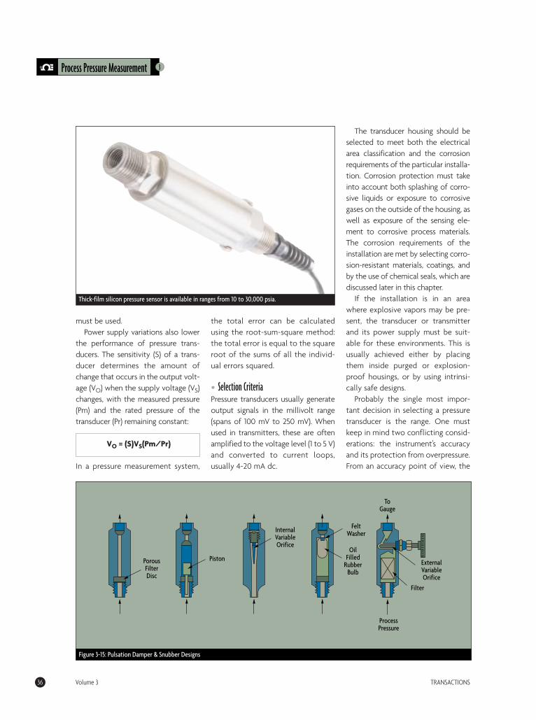
must be used.Power supply variations also lower
the performance of pressure trans-ducers. The sensitivity (S) of a trans-ducer determines the amount ofchange that occurs in the output volt-age (VO) when the supply voltage (VS)changes, with the measured pressure(Pm) and the rated pressure of thetransducer (Pr) remaining constant:
VO = (S)VS(Pm/Pr)
In a pressure measurement system,
the total error can be calculatedusing the root-sum-square method:the total error is equal to the squareroot of the sums of all the individ-ual errors squared.
• Selection CriteriaPressure transducers usually generateoutput signals in the millivolt range(spans of 100 mV to 250 mV). Whenused in transmitters, these are oftenamplified to the voltage level (1 to 5 V)and converted to current loops,usually 4-20 mA dc.
The transducer housing should beselected to meet both the electricalarea classification and the corrosionrequirements of the particular installa-tion. Corrosion protection must takeinto account both splashing of corro-sive liquids or exposure to corrosivegases on the outside of the housing, aswell as exposure of the sensing ele-ment to corrosive process materials.The corrosion requirements of theinstallation are met by selecting corro-sion-resistant materials, coatings, andby the use of chemical seals, which arediscussed later in this chapter.
If the installation is in an areawhere explosive vapors may be pre-sent, the transducer or transmitterand its power supply must be suit-able for these environments. This isusually achieved either by placingthem inside purged or explosion-proof housings, or by using intrinsi-cally safe designs.
Probably the single most impor-tant decision in selecting a pressuretransducer is the range. One mustkeep in mind two conflicting consid-erations: the instrument’s accuracyand its protection from overpressure.From an accuracy point of view, the
3Process Pressure Measurement
36 Volume 3 TRANSACTIONS
Porous Filter Disc
Piston
Internal Variable Orifice
Oil Filled
Rubber Bulb
Felt Washer
External Variable Orifice
Filter
Process Pressure
To Gauge
Figure 3-15: Pulsation Damper & Snubber Designs
Thick-film silicon pressure sensor is available in ranges from 10 to 30,000 psia.
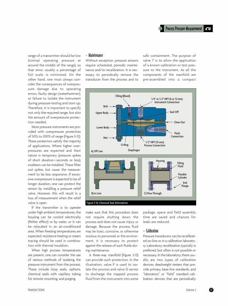
range of a transmitter should be low(normal operating pressure ataround the middle of the range), sothat error, usually a percentage offull scale, is minimized. On theother hand, one must always con-sider the consequences of overpres-sure damage due to operatingerrors, faulty design (waterhammer),or failure to isolate the instrumentduring pressure-testing and start-up.Therefore, it is important to specifynot only the required range, but alsothe amount of overpressure protec-tion needed.
Most pressure instruments are pro-vided with overpressure protectionof 50% to 200% of range (Figure 3-12).These protectors satisfy the majorityof applications. Where higher over-pressures are expected and theirnature is temporary (pressure spikesof short duration—seconds or less),snubbers can be installed. These filterout spikes, but cause the measure-ment to be less responsive. If exces-sive overpressure is expected to be oflonger duration, one can protect thesensor by installing a pressure reliefvalve. However, this will result in aloss of measurement when the reliefvalve is open.
If the transmitter is to operateunder high ambient temperatures, thehousing can be cooled electrically(Peltier effect) or by water, or it canbe relocated in an air-conditionedarea. When freezing temperatures areexpected, resistance heating or steamtracing should be used in combina-tion with thermal insulation.
When high process temperaturesare present, one can consider the useof various methods of isolating thepressure instrument from the process.These include loop seals, siphons,chemical seals with capillary tubingfor remote mounting, and purging.
• MaintenanceWithout exception, pressure sensorsrequire scheduled, periodic mainte-nance and/or recalibration. It is nec-essary to periodically remove thetransducer from the process and to
make sure that this procedure doesnot require shutting down theprocess and does not cause injury ordamage. Because the process fluidmay be toxic, corrosive, or otherwisenoxious to personnel or the environ-ment, it is necessary to protectagainst the release of such fluids dur-ing maintenance.
A three-way manifold (Figure 3-13)can provide such protection. In theillustration, valve P is used to iso-late the process and valve D servesto discharge the trapped processfluid from the instrument into some
safe containment. The purpose ofvalve T is to allow the applicationof a known calibration or test pres-sure to the instrument. As all thecomponents of the manifold arepre-assembled into a compact
package, space and field assemblytime are saved and chances forleaks are reduced.
• CalibrationPressure transducers can be recalibrat-ed on-line or in a calibration laborato-ry. Laboratory recalibration typically ispreferred, but often is not possible ornecessary. In the laboratory, there usu-ally are two types of calibrationdevices: deadweight testers that pro-vide primary, base-line standards, and“laboratory” or “field” standard cali-bration devices that are periodically
3 Process Pressure Measurement
TRANSACTIONS Volume 3 37
Figure 3-16: Chemical Seal Alternatives
A) Off Line
B) In Line
HousingFilling Fluid
Flexible Cylinder
End Flange
C) Flow-Through
1/4" or 1/2" NPT (6 or 13 mm) Instrument Connection
Clean Out
Seal-Off
Flush Connection
1/2" NPT (13 mm) Process Connection
Nut
Lower Body
Upper Body
Bolt
Filling (Bleed)
O-Ring
Diaphragm
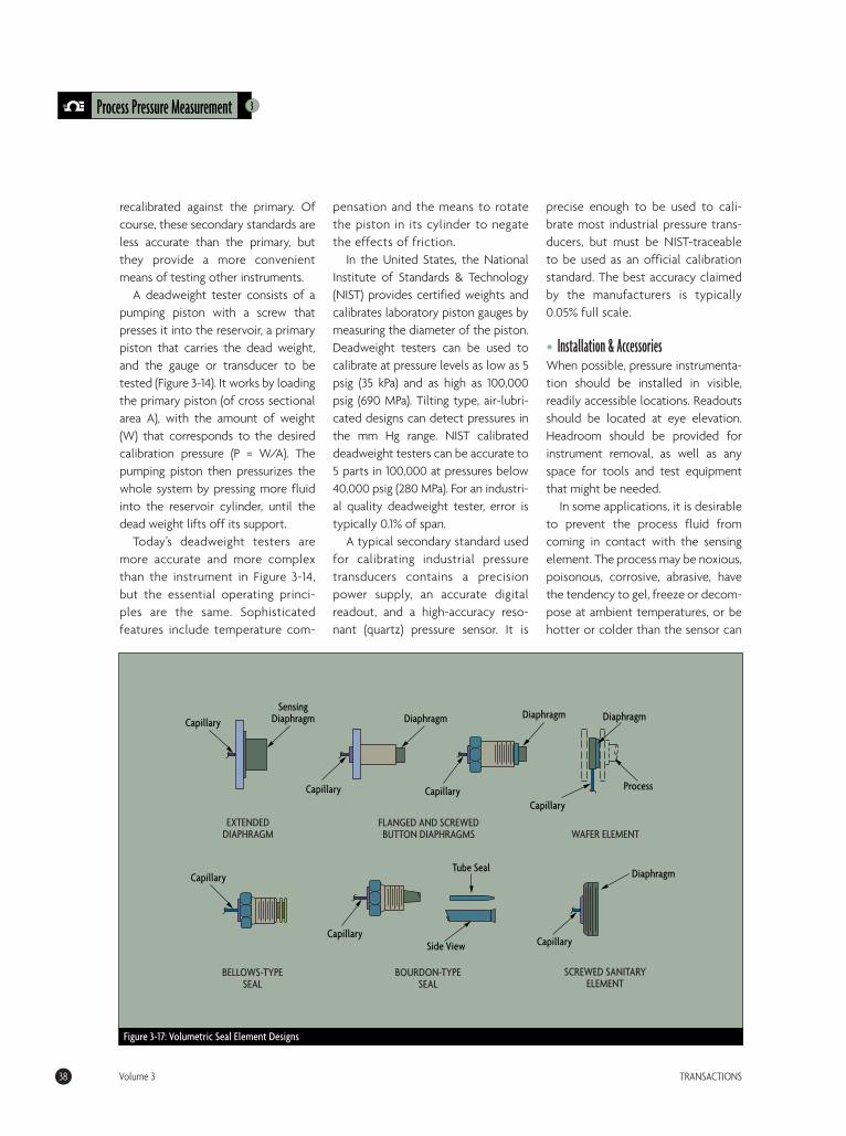
recalibrated against the primary. Ofcourse, these secondary standards areless accurate than the primary, butthey provide a more convenientmeans of testing other instruments.
A deadweight tester consists of apumping piston with a screw thatpresses it into the reservoir, a primarypiston that carries the dead weight,and the gauge or transducer to betested (Figure 3-14). It works by loadingthe primary piston (of cross sectionalarea A), with the amount of weight(W) that corresponds to the desiredcalibration pressure (P = W/A). Thepumping piston then pressurizes thewhole system by pressing more fluidinto the reservoir cylinder, until thedead weight lifts off its support.
Today’s deadweight testers aremore accurate and more complexthan the instrument in Figure 3-14,but the essential operating princi-ples are the same. Sophisticatedfeatures include temperature com-
pensation and the means to rotatethe piston in its cylinder to negatethe effects of friction.
In the United States, the NationalInstitute of Standards & Technology(NIST) provides certified weights andcalibrates laboratory piston gauges bymeasuring the diameter of the piston.Deadweight testers can be used tocalibrate at pressure levels as low as 5psig (35 kPa) and as high as 100,000psig (690 MPa). Tilting type, air-lubri-cated designs can detect pressures inthe mm Hg range. NIST calibrateddeadweight testers can be accurate to5 parts in 100,000 at pressures below40,000 psig (280 MPa). For an industri-al quality deadweight tester, error istypically 0.1% of span.
A typical secondary standard usedfor calibrating industrial pressuretransducers contains a precisionpower supply, an accurate digitalreadout, and a high-accuracy reso-nant (quartz) pressure sensor. It is
precise enough to be used to cali-brate most industrial pressure trans-ducers, but must be NIST-traceableto be used as an official calibrationstandard. The best accuracy claimedby the manufacturers is typically0.05% full scale.
• Installation & AccessoriesWhen possible, pressure instrumenta-tion should be installed in visible,readily accessible locations. Readoutsshould be located at eye elevation.Headroom should be provided forinstrument removal, as well as anyspace for tools and test equipmentthat might be needed.
In some applications, it is desirableto prevent the process fluid fromcoming in contact with the sensingelement. The process may be noxious,poisonous, corrosive, abrasive, havethe tendency to gel, freeze or decom-pose at ambient temperatures, or behotter or colder than the sensor can
3Process Pressure Measurement
38 Volume 3 TRANSACTIONS
CapillarySensing
Diaphragm
EXTENDED DIAPHRAGM
FLANGED AND SCREWED BUTTON DIAPHRAGMS
BELLOWS-TYPE SEAL
BOURDON-TYPE SEAL
SCREWED SANITARY ELEMENT
DiaphragmCapillary
Capillary
Diaphragm
Capillary
Diaphragm
Capillary Process
WAFER ELEMENT
Diaphragm
Capillary
Capillary
Tube Seal
Side View
Figure 3-17: Volumetric Seal Element Designs
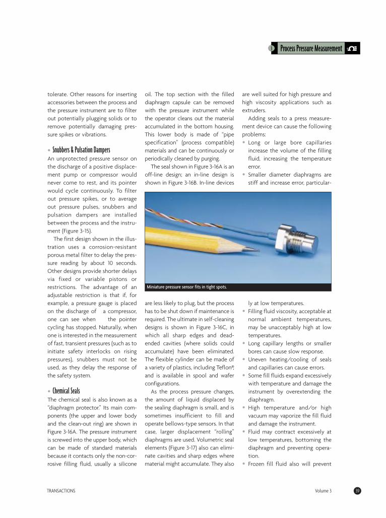
tolerate. Other reasons for insertingaccessories between the process andthe pressure instrument are to filterout potentially plugging solids or toremove potentially damaging pres-sure spikes or vibrations.
• Snubbers & Pulsation DampersAn unprotected pressure sensor onthe discharge of a positive displace-ment pump or compressor wouldnever come to rest, and its pointerwould cycle continuously. To filterout pressure spikes, or to averageout pressure pulses, snubbers andpulsation dampers are installedbetween the process and the instru-ment (Figure 3-15).
The first design shown in the illus-tration uses a corrosion-resistantporous metal filter to delay the pres-sure reading by about 10 seconds.Other designs provide shorter delaysvia fixed or variable pistons orrestrictions. The advantage of anadjustable restriction is that if, forexample, a pressure gauge is placedon the discharge of a compressor,one can see when the pointercycling has stopped. Naturally, whenone is interested in the measurementof fast, transient pressures (such as toinitiate safety interlocks on risingpressures), snubbers must not beused, as they delay the response ofthe safety system.
• Chemical SealsThe chemical seal is also known as a“diaphragm protector.” Its main com-ponents (the upper and lower bodyand the clean-out ring) are shown inFigure 3-16A. The pressure instrumentis screwed into the upper body, whichcan be made of standard materialsbecause it contacts only the non-cor-rosive filling fluid, usually a silicone
oil. The top section with the filleddiaphragm capsule can be removedwith the pressure instrument whilethe operator cleans out the materialaccumulated in the bottom housing.This lower body is made of “pipespecification” (process compatible)materials and can be continuously orperiodically cleaned by purging.
The seal shown in Figure 3-16A is anoff-line design; an in-line design isshown in Figure 3-16B. In-line devices
are less likely to plug, but the processhas to be shut down if maintenance isrequired. The ultimate in self-cleaningdesigns is shown in Figure 3-16C, inwhich all sharp edges and dead-ended cavities (where solids couldaccumulate) have been eliminated.The flexible cylinder can be made ofa variety of plastics, including Teflon®,and is available in spool and waferconfigurations.
As the process pressure changes,the amount of liquid displaced bythe sealing diaphragm is small, and issometimes insufficient to fill andoperate bellows-type sensors. In thatcase, larger displacement “rolling”diaphragms are used. Volumetric sealelements (Figure 3-17) also can elimi-nate cavities and sharp edges wherematerial might accumulate. They also
are well suited for high pressure andhigh viscosity applications such asextruders.
Adding seals to a press measure-ment device can cause the followingproblems:• Long or large bore capillaries
increase the volume of the fillingfluid, increasing the temperatureerror.
• Smaller diameter diaphragms arestiff and increase error, particular-
ly at low temperatures. • Filling fluid viscosity, acceptable at
normal ambient temperatures,may be unacceptably high at lowtemperatures.
• Long capillary lengths or smallerbores can cause slow response.
• Uneven heating/cooling of sealsand capillaries can cause errors.
• Some fill fluids expand excessivelywith temperature and damage theinstrument by overextending thediaphragm.
• High temperature and/or highvacuum may vaporize the fill fluidand damage the instrument.
• Fluid may contract excessively atlow temperatures, bottoming thediaphragm and preventing opera-tion.
• Frozen fill fluid also will prevent
3 Process Pressure Measurement
TRANSACTIONS Volume 3 39
Miniature pressure sensor fits in tight spots.
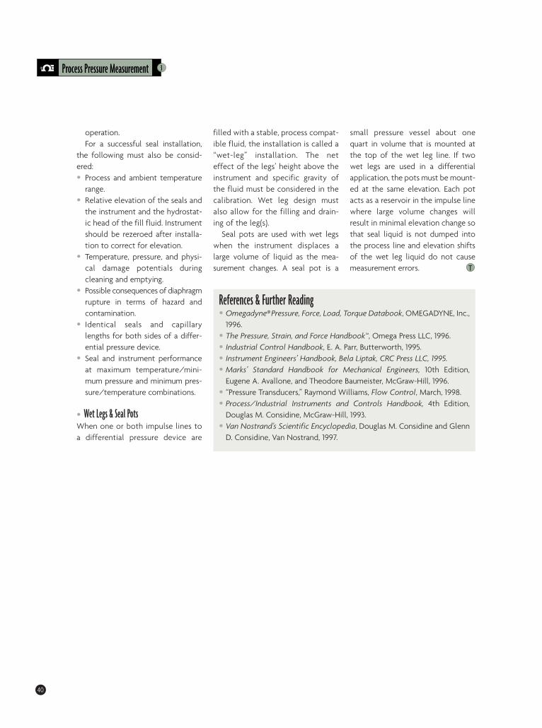
operation.For a successful seal installation,
the following must also be consid-ered: • Process and ambient temperature
range.• Relative elevation of the seals and
the instrument and the hydrostat-ic head of the fill fluid. Instrumentshould be rezeroed after installa-tion to correct for elevation.
• Temperature, pressure, and physi-cal damage potentials duringcleaning and emptying.
• Possible consequences of diaphragmrupture in terms of hazard andcontamination.
• Identical seals and capillarylengths for both sides of a differ-ential pressure device.
• Seal and instrument performanceat maximum temperature/mini-mum pressure and minimum pres-sure/temperature combinations.
• Wet Legs & Seal PotsWhen one or both impulse lines toa differential pressure device are
filled with a stable, process compat-ible fluid, the installation is called a“wet-leg” installation. The neteffect of the legs’ height above theinstrument and specific gravity ofthe fluid must be considered in thecalibration. Wet leg design mustalso allow for the filling and drain-ing of the leg(s).
Seal pots are used with wet legswhen the instrument displaces alarge volume of liquid as the mea-surement changes. A seal pot is a
small pressure vessel about onequart in volume that is mounted atthe top of the wet leg line. If twowet legs are used in a differentialapplication, the pots must be mount-ed at the same elevation. Each potacts as a reservoir in the impulse linewhere large volume changes willresult in minimal elevation change sothat seal liquid is not dumped intothe process line and elevation shiftsof the wet leg liquid do not causemeasurement errors. T
3Process Pressure Measurement
40
References & Further Reading• Omegadyne®Pressure, Force, Load, Torque Databook, OMEGADYNE, Inc.,
1996.• The Pressure, Strain, and Force Handbook™, Omega Press LLC, 1996.• Industrial Control Handbook, E. A. Parr, Butterworth, 1995.• Instrument Engineers’ Handbook, Bela Liptak, CRC Press LLC, 1995.• Marks’ Standard Handbook for Mechanical Engineers, 10th Edition,
Eugene A. Avallone, and Theodore Baumeister, McGraw-Hill, 1996.• “Pressure Transducers,” Raymond Williams, Flow Control, March, 1998.• Process/Industrial Instruments and Controls Handbook, 4th Edition,
Douglas M. Considine, McGraw-Hill, 1993.• Van Nostrand’s Scientific Encyclopedia, Douglas M. Considine and Glenn
D. Considine, Van Nostrand, 1997.
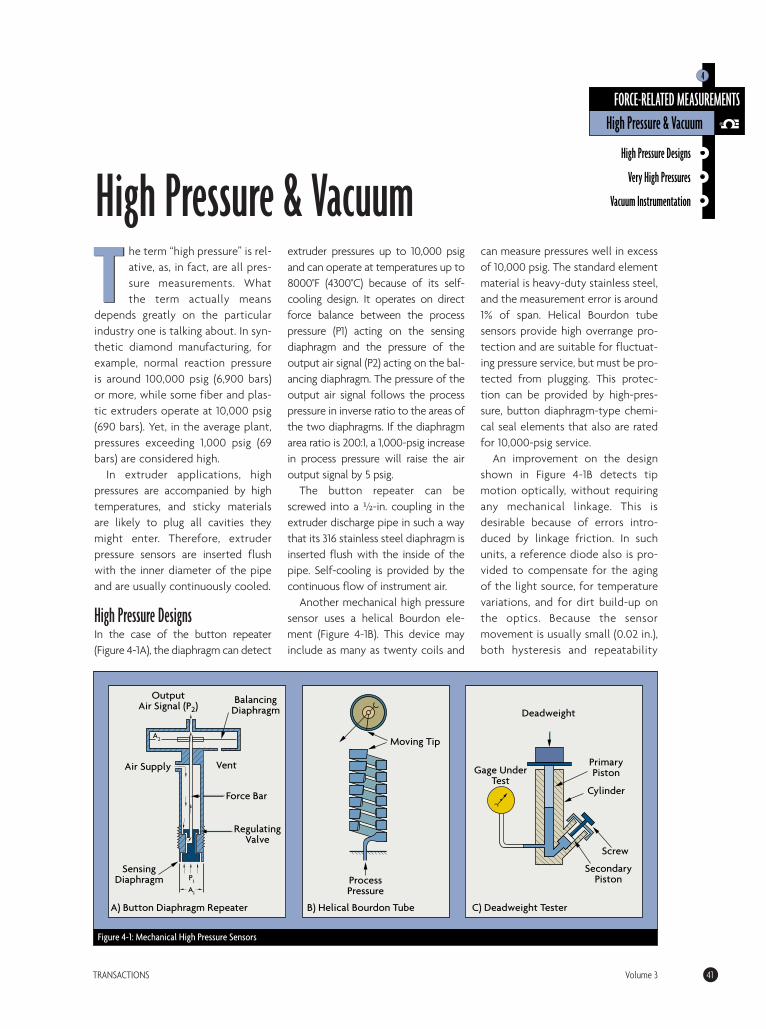
The term “high pressure” is rel-ative, as, in fact, are all pres-sure measurements. Whatthe term actually means
depends greatly on the particularindustry one is talking about. In syn-thetic diamond manufacturing, forexample, normal reaction pressureis around 100,000 psig (6,900 bars)or more, while some fiber and plas-tic extruders operate at 10,000 psig(690 bars). Yet, in the average plant,pressures exceeding 1,000 psig (69bars) are considered high.
In extruder applications, highpressures are accompanied by hightemperatures, and sticky materialsare likely to plug all cavities theymight enter. Therefore, extruderpressure sensors are inserted flushwith the inner diameter of the pipeand are usually continuously cooled.
High Pressure DesignsIn the case of the button repeater(Figure 4-1A), the diaphragm can detect
extruder pressures up to 10,000 psigand can operate at temperatures up to8000°F (4300°C) because of its self-cooling design. It operates on directforce balance between the processpressure (P1) acting on the sensingdiaphragm and the pressure of theoutput air signal (P2) acting on the bal-ancing diaphragm. The pressure of theoutput air signal follows the processpressure in inverse ratio to the areas ofthe two diaphragms. If the diaphragmarea ratio is 200:1, a 1,000-psig increasein process pressure will raise the airoutput signal by 5 psig.
The button repeater can bescrewed into a H-in. coupling in theextruder discharge pipe in such a waythat its 316 stainless steel diaphragm isinserted flush with the inside of thepipe. Self-cooling is provided by thecontinuous flow of instrument air.
Another mechanical high pressuresensor uses a helical Bourdon ele-ment (Figure 4-1B). This device mayinclude as many as twenty coils and
can measure pressures well in excessof 10,000 psig. The standard elementmaterial is heavy-duty stainless steel,and the measurement error is around1% of span. Helical Bourdon tubesensors provide high overrange pro-tection and are suitable for fluctuat-ing pressure service, but must be pro-tected from plugging. This protec-tion can be provided by high-pres-sure, button diaphragm-type chemi-cal seal elements that also are ratedfor 10,000-psig service.
An improvement on the designshown in Figure 4-1B detects tipmotion optically, without requiringany mechanical linkage. This isdesirable because of errors intro-duced by linkage friction. In suchunits, a reference diode also is pro-vided to compensate for the agingof the light source, for temperaturevariations, and for dirt build-up onthe optics. Because the sensormovement is usually small (0.02 in.),both hysteresis and repeatability
TRANSACTIONS Volume 3 41
THigh Pressure & Vacuum
Figure 4-1: Mechanical High Pressure Sensors
Output Air Signal (P2)
A) Button Diaphragm Repeater B) Helical Bourdon Tube C) Deadweight Tester
Balancing Diaphragm
Vent
Force Bar
Regulating Valve
Sensing Diaphragm
AI
PI
A2
Air Supply
Process Pressure
Moving Tip
Primary PistonGage Under
Test
Deadweight
Screw
Secondary Piston
Cylinder
High Pressure Designs
Very High Pressures
Vacuum Instrumentation
FORCE-RELATED MEASUREMENTSHigh Pressure & Vacuum
4
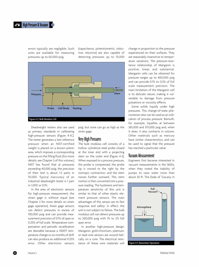
errors typically are negligible. Suchunits are available for measuringpressures up to 60,000 psig.
Deadweight testers also are usedas primary standards in calibratinghigh-pressure sensors (Figure 4-1C).The tester generates a test referencepressure when an NIST-certifiedweight is placed on a known pistonarea, which imposes a correspondingpressure on the filling fluid. (For moredetails, see Chapter 3 of this volume.)NIST has found that at pressuresexceeding 40,000 psig, the precisionof their test is about 1.5 parts in10,000. Typical inaccuracy of anindustrial deadweight tester is 1 partin 1,000 or 0.1%.
In the area of electronic sensorsfor high-pressure measurement, thestrain gage is without equal (seeChapter 2 for more details on straingage operation). Strain gage sensorscan detect pressures in excess of100,000 psig and can provide mea-surement precision of 0.1% of span or0.25% of full scale. Temperature com-pensation and periodic recalibrationare desirable because a 1000°F tem-perature change or six months of driftcan also produce an additional 0.25%error. Other electronic sensors
(capacitance, potentiometric, induc-tive, reluctive) are also capable ofdetecting pressures up to 10,000
psig, but none can go as high as thestrain gage.
Very High PressuresThe bulk modulus cell consists of ahollow cylindrical steel probe closedat the inner end with a projectingstem on the outer end (Figure 4-2).When exposed to a process pressure,the probe is compressed, the probetip is moved to the right by theisotropic contraction, and the stemmoves further outward. This stemmotion is then converted into a pres-sure reading. The hysteresis and tem-perature sensitivity of this unit issimilar to that of other elastic ele-ment pressure sensors. The mainadvantages of this sensor are its fastresponse and safety: in effect, theunit is not subject to failure. The bulkmodulus cell can detect pressures upto 200,000 psig with 1% to 2% fullspan error.
In another high-pressure design,Manganin, gold-chromium, platinum,or lead wire sensors are wound heli-cally on a core. The electrical resis-tance of these wire materials will
change in proportion to the pressureexperienced on their surfaces. Theyare reasonably insensitive to temper-ature variations. The pressure-resis-tance relationship of Manganin ispositive, linear, and substantial.Manganin cells can be obtained forpressure ranges up to 400,000 psigand can provide 0.1% to 0.5% of fullscale measurement precision. Themain limitation of the Manganin cellis its delicate nature, making it vul-nerable to damage from pressurepulsations or viscosity effects.
Some solids liquefy under highpressures. This change-of-state phe-nomenon also can be used as an indi-cation of process pressure. Bismuth,for example, liquefies at between365,000 and 375,000 psig and, whenit does, it also contracts in volume.Other materials such as mercuryhave similar characteristics, and canbe used to signal that the pressurehas reached a particular value.
Vacuum MeasurementEngineers first became interested invacuum measurements in the 1600s,when they noted the inability ofpumps to raise water more thanabout 30 ft. The Duke of Tuscany in
4High Pressure & Vacuum
42 Volume 3 TRANSACTIONS
Figure 4-2: Bulk Modulus Cell
Stem
PackingCell BodyProbe
Pressure
Figure 4-3: Barometer Operation
Atmosphere
Full Vacuum

Italy commissioned Galileo to inves-tigate the “problem.” Galileo, amongothers, also devised a number ofexperiments to investigate theproperties of air. Among the toolsused for these experiments werepistons to measure force and awater barometer (about 34 ft. tall)
to measure vacuum pressure. After Galileo’s death in 1642,
Evangelista Torricelli carried on thework of vacuum-related investiga-tion and invented the mercurybarometer (Figure 4-3). He discoveredthat the atmosphere exerts a force of14.7 lb. per square in. (psi) and that,inside a fully evacuated tube, thepressure was enough to raise a col-umn of mercury to a height of 29.9 in.
(760 mm). The height of a mercurycolumn is therefore a direct measureof the atmospheric pressure.
In 1644, French mathematicianBlaise Pascal asked a group ofmountaineers to carry a barometerinto the Alps and proved that airpressure decreases with altitude.
The average barometric pressure atsea level can balance the height of a760 mm mercury column, and thispressure is defined as a standardAtmosphere. The value for 1/760thof an atmosphere is called a torr, inhonor of Torricelli.
In 1872, McLeod invented theMcLeod vacuum detector gauge,which measures the pressure of agas by measuring its volume twice,
once at the unknown low pressureand again at a higher reference pres-sure. The pressurized new volume isthen an indication of the initialabsolute pressure. Versions of theMcLeod Gauge continue to be usedtoday as a standard for calibratingvacuum gauges.
• ApplicationsVacuum gauges in use today fall intothree main categories: mechanical,thermal, and ionization. Their pres-sure ranges are given in Figure 4-4. Ingeneral, for high vacuum services(around 10-6 torr), either cold cathodeor Bayard-Alpert hot cathode gaugesare suitable. Neither is particularlyaccurate or stable, and both requirefrequent calibration.
4 High Pressure & Vacuum
TRANSACTIONS Volume 3 43
Figure 4-4: Vacuum Gauge Measurement Ranges
Bourdon
Bellows
Diaphragm
Quartz Helix
Liquid Manometer
Molecular Momentum
Capacitance Diaphragm
McLeod Gage
Viscuous Friction of Spinning Ball
Pirani (Thermistor)
Thermocouple, Thermopile
Convectron Gage
Hot Cathode (Schultz-Phelps)
Hot Cathode (Bayard-Alpert)
Cold Cathode (Philips)
Cold Cathode (Redhead)
10-12 10-11 10-10 10-9 10-8 10-7 10-6 10-5 10-4 10-3 10-2 10-1 1 10 100 1000
Mechanical
Thermal
Ionization
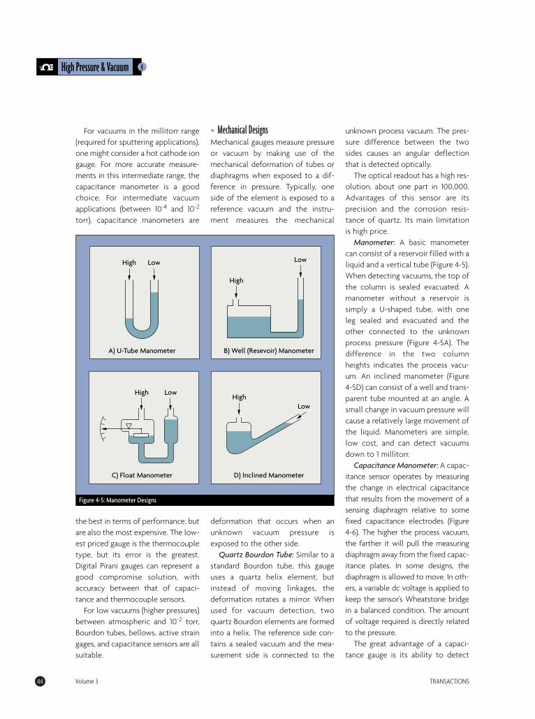
For vacuums in the millitorr range(required for sputtering applications),one might consider a hot cathode iongauge. For more accurate measure-ments in this intermediate range, thecapacitance manometer is a goodchoice. For intermediate vacuumapplications (between 10-4 and 10-2
torr), capacitance manometers are
the best in terms of performance, butare also the most expensive. The low-est priced gauge is the thermocoupletype, but its error is the greatest.Digital Pirani gauges can represent agood compromise solution, withaccuracy between that of capaci-tance and thermocouple sensors.
For low vacuums (higher pressures)between atmospheric and 10-2 torr,Bourdon tubes, bellows, active straingages, and capacitance sensors are allsuitable.
• Mechanical DesignsMechanical gauges measure pressureor vacuum by making use of themechanical deformation of tubes ordiaphragms when exposed to a dif-ference in pressure. Typically, oneside of the element is exposed to areference vacuum and the instru-ment measures the mechanical
deformation that occurs when anunknown vacuum pressure isexposed to the other side.
Quartz Bourdon Tube: Similar to astandard Bourdon tube, this gaugeuses a quartz helix element, butinstead of moving linkages, thedeformation rotates a mirror. Whenused for vacuum detection, twoquartz Bourdon elements are formedinto a helix. The reference side con-tains a sealed vacuum and the mea-surement side is connected to the
unknown process vacuum. The pres-sure difference between the twosides causes an angular deflectionthat is detected optically.
The optical readout has a high res-olution, about one part in 100,000.Advantages of this sensor are itsprecision and the corrosion resis-tance of quartz. Its main limitationis high price.
Manometer: A basic manometercan consist of a reservoir filled with aliquid and a vertical tube (Figure 4-5).When detecting vacuums, the top ofthe column is sealed evacuated. Amanometer without a reservoir issimply a U-shaped tube, with oneleg sealed and evacuated and theother connected to the unknownprocess pressure (Figure 4-5A). Thedifference in the two columnheights indicates the process vacu-um. An inclined manometer (Figure4-5D) can consist of a well and trans-parent tube mounted at an angle. Asmall change in vacuum pressure willcause a relatively large movement ofthe liquid. Manometers are simple,low cost, and can detect vacuumsdown to 1 millitorr.
Capacitance Manometer: A capac-itance sensor operates by measuringthe change in electrical capacitancethat results from the movement of asensing diaphragm relative to somefixed capacitance electrodes (Figure4-6). The higher the process vacuum,the farther it will pull the measuringdiaphragm away from the fixed capac-itance plates. In some designs, thediaphragm is allowed to move. In oth-ers, a variable dc voltage is applied tokeep the sensor’s Wheatstone bridgein a balanced condition. The amountof voltage required is directly relatedto the pressure.
The great advantage of a capaci-tance gauge is its ability to detect
4High Pressure & Vacuum
44 Volume 3 TRANSACTIONS
Figure 4-5: Manometer Designs
High
A) U-Tube Manometer
C) Float Manometer
B) Well (Resevoir) Manometer
D) Inclined Manometer
Low
High
Low
High LowHigh
Low
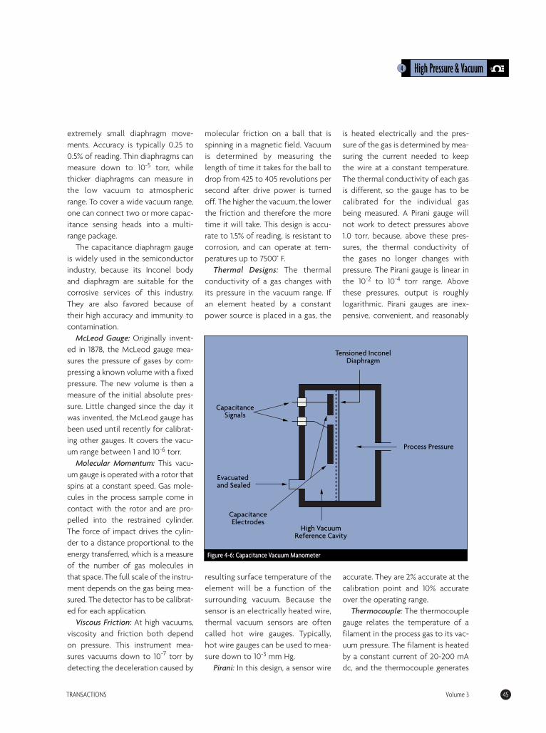
extremely small diaphragm move-ments. Accuracy is typically 0.25 to0.5% of reading. Thin diaphragms canmeasure down to 10-5 torr, whilethicker diaphragms can measure inthe low vacuum to atmosphericrange. To cover a wide vacuum range,one can connect two or more capac-itance sensing heads into a multi-range package.
The capacitance diaphragm gaugeis widely used in the semiconductorindustry, because its Inconel bodyand diaphragm are suitable for thecorrosive services of this industry.They are also favored because oftheir high accuracy and immunity tocontamination.
McLeod Gauge: Originally invent-ed in 1878, the McLeod gauge mea-sures the pressure of gases by com-pressing a known volume with a fixedpressure. The new volume is then ameasure of the initial absolute pres-sure. Little changed since the day itwas invented, the McLeod gauge hasbeen used until recently for calibrat-ing other gauges. It covers the vacu-um range between 1 and 10-6 torr.
Molecular Momentum: This vacu-um gauge is operated with a rotor thatspins at a constant speed. Gas mole-cules in the process sample come incontact with the rotor and are pro-pelled into the restrained cylinder.The force of impact drives the cylin-der to a distance proportional to theenergy transferred, which is a measureof the number of gas molecules inthat space. The full scale of the instru-ment depends on the gas being mea-sured. The detector has to be calibrat-ed for each application.
Viscous Friction: At high vacuums,viscosity and friction both dependon pressure. This instrument mea-sures vacuums down to 10-7 torr bydetecting the deceleration caused by
molecular friction on a ball that isspinning in a magnetic field. Vacuumis determined by measuring thelength of time it takes for the ball todrop from 425 to 405 revolutions persecond after drive power is turnedoff. The higher the vacuum, the lowerthe friction and therefore the moretime it will take. This design is accu-rate to 1.5% of reading, is resistant tocorrosion, and can operate at tem-peratures up to 7500° F.
Thermal Designs: The thermalconductivity of a gas changes withits pressure in the vacuum range. Ifan element heated by a constantpower source is placed in a gas, the
resulting surface temperature of theelement will be a function of thesurrounding vacuum. Because thesensor is an electrically heated wire,thermal vacuum sensors are oftencalled hot wire gauges. Typically,hot wire gauges can be used to mea-sure down to 10-3 mm Hg.
Pirani: In this design, a sensor wire
is heated electrically and the pres-sure of the gas is determined by mea-suring the current needed to keepthe wire at a constant temperature.The thermal conductivity of each gasis different, so the gauge has to becalibrated for the individual gasbeing measured. A Pirani gauge willnot work to detect pressures above1.0 torr, because, above these pres-sures, the thermal conductivity ofthe gases no longer changes withpressure. The Pirani gauge is linear inthe 10-2 to 10-4 torr range. Abovethese pressures, output is roughlylogarithmic. Pirani gauges are inex-pensive, convenient, and reasonably
accurate. They are 2% accurate at thecalibration point and 10% accurateover the operating range.
Thermocouple: The thermocouplegauge relates the temperature of afilament in the process gas to its vac-uum pressure. The filament is heatedby a constant current of 20-200 mAdc, and the thermocouple generates
4 High Pressure & Vacuum
TRANSACTIONS Volume 3 45
Figure 4-6: Capacitance Vacuum Manometer
Tensioned Inconel Diaphragm
Capacitance Signals
Process Pressure
Evacuated and Sealed
Capacitance Electrodes
High Vacuum Reference Cavity
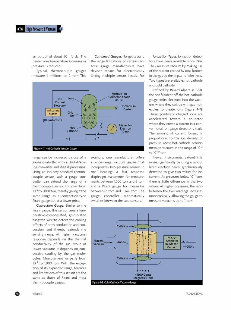
an output of about 20 mV dc. Theheater wire temperature increases aspressure is reduced.
Typical thermocouple gaugesmeasure 1 millitorr to 2 torr. This
range can be increased by use of agauge controller with a digital/ana-log converter and digital processing.Using an industry standard thermo-couple sensor, such a gauge con-troller can extend the range of athermocouple sensor to cover from10-3 to 1,000 torr, thereby giving it thesame range as a convection-typePirani gauge but at a lower price.
Convection Gauge: Similar to thePirani gauge, this sensor uses a tem-perature-compensated, gold-platedtungsten wire to detect the coolingeffects of both conduction and con-vection, and thereby extends thesensing range. At higher vacuums,response depends on the thermalconductivity of the gas, while atlower vacuums it depends on con-vective cooling by the gas mole-cules. Measurement range is from10-3 to 1,000 torr. With the excep-tion of its expanded range, featuresand limitations of this sensor are thesame as those of Pirani and mostthermocouple gauges.
Combined Gauges: To get aroundthe range limitations of certain sen-sors, gauge manufacturers havedevised means for electronicallylinking multiple sensor heads. For
example, one manufacturer offersa wide-range vacuum gauge thatincorporates two pressure sensors inone housing: a fast responsediaphragm manometer for measure-ments between 1,500 torr and 2 torr,and a Pirani gauge for measuringbetween 2 torr and 1 millitorr. Thegauge controller automaticallyswitches between the two sensors.
Ionization Types: Ionization detec-tors have been available since 1916.They measure vacuum by making useof the current carried by ions formedin the gas by the impact of electrons.Two types are available: hot cathodeand cold cathode.
Refined by Bayard-Alpert in 1950,the hot filament off the hot-cathodegauge emits electrons into the vacu-um, where they collide with gas mol-ecules to create ions (Figure 4-7).These positively charged ions areaccelerated toward a collectorwhere they create a current in a con-ventional ion gauge detector circuit.The amount of current formed isproportional to the gas density orpressure. Most hot-cathode sensorsmeasure vacuum in the range of 10-2
to 10-10 torr.Newer instruments extend this
range significantly by using a modu-lated electron beam, synchronouslydetected to give two values for ioncurrent. At pressures below 10-3 torr,there is little difference in the twovalues. At higher pressures, the ratiobetween the two readings increasesmonotonically, allowing the gauge tomeasure vacuums up to 1 torr.
4High Pressure & Vacuum
46 Volume 3 TRANSACTIONS
Figure 4-8: Cold-Cathode Vacuum Gauge
Process Vacuum
Cathode
Anode
~1500 Gauss Magnetic Field
-Micro-
Ammeter Reads the
Vacuum ~4000 V
+
Cathode
Figure 4-7: Hot-Cathode Vacuum Gauge
IonsPositive Ion
Collector Anode @ - 30
To Vacuum System
Meter For Electron (10 mA)
Grid + 150V
(100 mA/torr)
Hot Cathode
++
Ion Current
Detector
-
++
+ ++
- - ----
- -
Indicating Meter
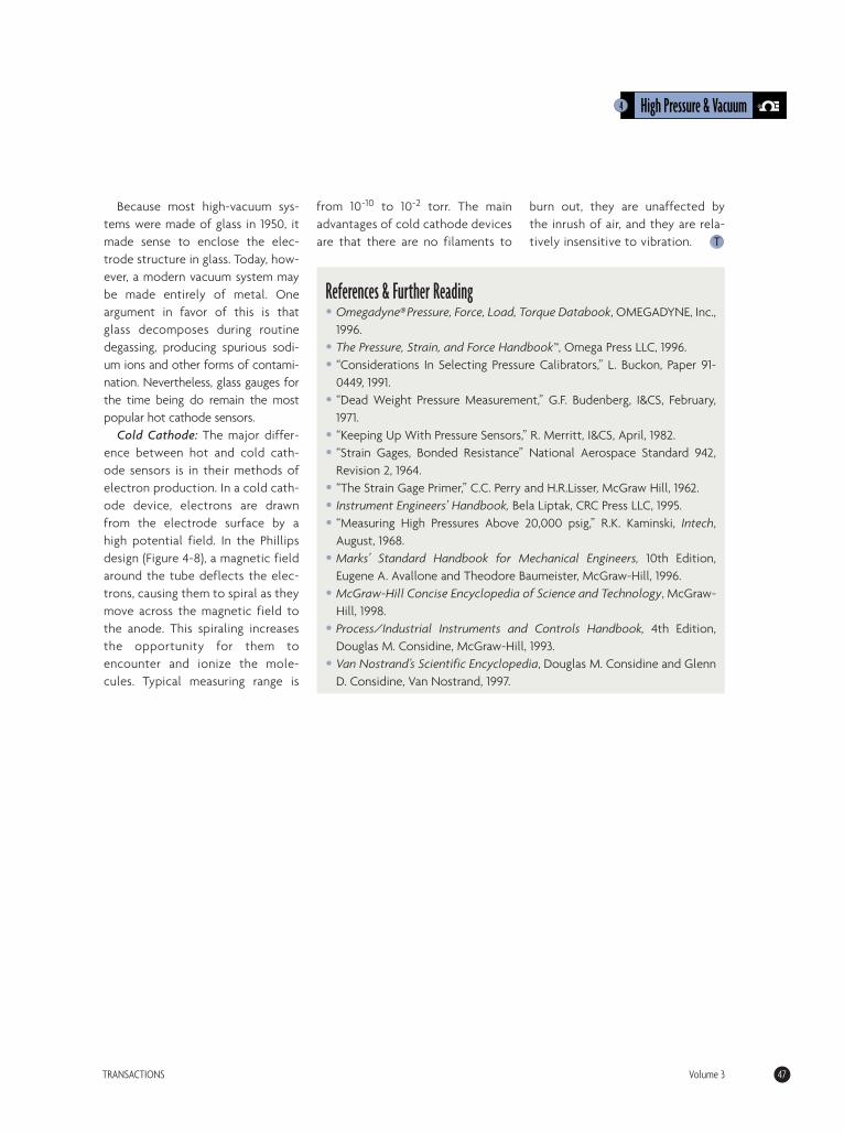
Because most high-vacuum sys-tems were made of glass in 1950, itmade sense to enclose the elec-trode structure in glass. Today, how-ever, a modern vacuum system maybe made entirely of metal. Oneargument in favor of this is thatglass decomposes during routinedegassing, producing spurious sodi-um ions and other forms of contami-nation. Nevertheless, glass gauges forthe time being do remain the mostpopular hot cathode sensors.
Cold Cathode: The major differ-ence between hot and cold cath-ode sensors is in their methods ofelectron production. In a cold cath-ode device, electrons are drawnfrom the electrode surface by ahigh potential field. In the Phillipsdesign (Figure 4-8), a magnetic fieldaround the tube deflects the elec-trons, causing them to spiral as theymove across the magnetic field tothe anode. This spiraling increasesthe opportunity for them toencounter and ionize the mole-cules. Typical measuring range is
from 10-10 to 10-2 torr. The mainadvantages of cold cathode devicesare that there are no filaments to
burn out, they are unaffected bythe inrush of air, and they are rela-tively insensitive to vibration. T
4 High Pressure & Vacuum
TRANSACTIONS Volume 3 47
References & Further Reading• Omegadyne®Pressure, Force, Load, Torque Databook, OMEGADYNE, Inc.,
1996.• The Pressure, Strain, and Force Handbook™, Omega Press LLC, 1996.• “Considerations In Selecting Pressure Calibrators,” L. Buckon, Paper 91-
0449, 1991.• “Dead Weight Pressure Measurement,” G.F. Budenberg, I&CS, February,
1971.• “Keeping Up With Pressure Sensors,” R. Merritt, I&CS, April, 1982.• “Strain Gages, Bonded Resistance” National Aerospace Standard 942,
Revision 2, 1964. • “The Strain Gage Primer,” C.C. Perry and H.R.Lisser, McGraw Hill, 1962.• Instrument Engineers’ Handbook, Bela Liptak, CRC Press LLC, 1995.• “Measuring High Pressures Above 20,000 psig,” R.K. Kaminski, Intech,
August, 1968.• Marks’ Standard Handbook for Mechanical Engineers, 10th Edition,
Eugene A. Avallone and Theodore Baumeister, McGraw-Hill, 1996.• McGraw-Hill Concise Encyclopedia of Science and Technology, McGraw-
Hill, 1998.• Process/Industrial Instruments and Controls Handbook, 4th Edition,
Douglas M. Considine, McGraw-Hill, 1993.• Van Nostrand’s Scientific Encyclopedia, Douglas M. Considine and Glenn
D. Considine, Van Nostrand, 1997.
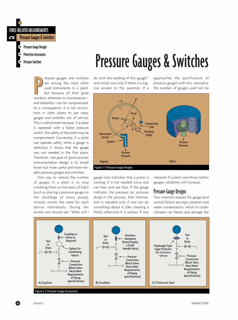
Pressure gauges and switchesare among the most oftenused instruments in a plant.But because of their great
numbers, attention to maintenance—and reliability—can be compromised.As a consequence, it is not uncom-mon in older plants to see manygauges and switches out of service.This is unfortunate because, if a plantis operated with a failed pressureswitch, the safety of the plant may becompromised. Conversely, if a plantcan operate safely while a gauge isdefective, it shows that the gaugewas not needed in the first place.Therefore, one goal of good processinstrumentation design is to installfewer but more useful and more reli-able pressure gauges and switches.
One way to reduce the numberof gauges in a plant is to stopinstalling them on the basis of habit(such as placing a pressure gauge onthe discharge of every pump).Instead, review the need for eachdevice individually. During thereview one should ask: “What will I
do with the reading of this gauge?”and install one only if there is a log-ical answer to the question. If a
gauge only indicates that a pump isrunning, it is not needed, since onecan hear and see that. If the gaugeindicates the pressure (or pressuredrop) in the process, that informa-tion is valuable only if one can dosomething about it (like cleaning afilter); otherwise it is useless. If one
approaches the specification ofpressure gauges with this mentality,the number of gauges used will be
reduced. If a plant uses fewer, bettergauges, reliability will increase.
Pressure Gauge DesignsTwo common reasons for gauge (andswitch) failure are pipe vibration andwater condensation, which in colderclimates can freeze and damage the
48 Volume 3 TRANSACTIONS
Pressure Gauge Designs
Protective Accessories
Pressure Switches
FORCE-RELATED MEASUREMENTSPressure Gauges & Switches
5
PPressure Gauges & Switches
Figure 5-1: Pressure Gauge Designs
µ
Process Pressure
A
A
Pivot
Connecting Link
Traveling Angle
Socket
Movement Sector
Pinion
Regular Filled
Process Pressure
Figure 5-2: Pressure Gauge Accessories
Test or
Drain
Coupling or Union as Required
Pulsation Dampener
(Some Employ a Small
Needle Valve)Diaphragm-Type Gage Protector For Corrosive
Service Pressure Connection (Block Valve Must Meet
Requirements of Piping
Specifications)
Pressure Connection (Block Valve Must Meet
Requirements of Piping
Specifications)
Pressure Connection (Block Valve Must Meet
Requirements of Piping
Specifications)
Siphon for Condensing
Vapors
Test or
Drain
Test or
Drain
A) Syphon B) Snubber C) Chemical Seal
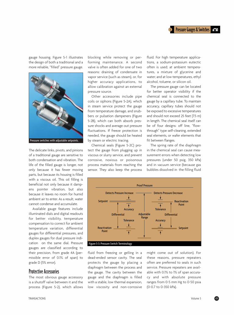
gauge housing. Figure 5-1 illustratesthe design of both a traditional and amore reliable, “filled” pressure gauge.
The delicate links, pivots, and pinionsof a traditional gauge are sensitive toboth condensation and vibration. Thelife of the filled gauge is longer, notonly because it has fewer movingparts, but because its housing is filledwith a viscous oil. This oil filling isbeneficial not only because it damp-ens pointer vibration, but alsobecause it leaves no room for humidambient air to enter. As a result, watercannot condense and accumulate.
Available gauge features includeilluminated dials and digital readoutsfor better visibility, temperaturecompensation to correct for ambienttemperature variation, differentialgauges for differential pressures, andduplex gauges for dual pressure indi-cation on the same dial. Pressuregauges are classified according totheir precision, from grade 4A (per-missible error of 0.1% of span) tograde D (5% error).
Protective AccessoriesThe most obvious gauge accessoryis a shutoff valve between it and theprocess (Figure 5-2), which allows
blocking while removing or per-forming maintenance. A secondvalve is often added for one of tworeasons: draining of condensate invapor service (such as steam), or, forhigher accuracy applications, toallow calibration against an externalpressure source.
Other accessories include pipecoils or siphons (Figure 5-2A), whichin steam service protect the gaugefrom temperature damage, and snub-bers or pulsation dampeners (Figure5-2B), which can both absorb pres-sure shocks and average out pressurefluctuations. If freeze protection isneeded, the gauge should be heatedby steam or electric tracing.
Chemical seals (Figure 5-2C) pro-tect the gauge from plugging up inviscous or slurry service, and preventcorrosive, noxious or poisonousprocess materials from reaching thesensor. They also keep the process
fluid from freezing or gelling in adead-ended sensor cavity. The sealprotects the gauge by placing adiaphragm between the process andthe gauge. The cavity between thegauge and the diaphragm is filledwith a stable, low thermal expansion,low viscosity and non-corrosive
fluid. For high temperature applica-tions, a sodium-potassium eutecticoften is used; at ambient tempera-tures, a mixture of glycerine andwater; and at low temperatures, ethylalcohol, toluene, or silicon oil.
The pressure gauge can be locatedfor better operator visibility if thechemical seal is connected to thegauge by a capillary tube. To maintainaccuracy, capillary tubes should notbe exposed to excessive temperaturesand should not exceed 25 feet (7.5 m)in length. The chemical seal itself canbe of four designs: off line, “flow-through” type self-cleaning, extendedseal elements, or wafer elements thatfit between flanges.
The spring rate of the diaphragmin the chemical seal can cause mea-surement errors when detecting lowpressures (under 50 psig, 350 kPa)and in vacuum service (because gasbubbles dissolved in the filling fluid
might come out of solution). Forthese reasons, pressure repeatersoften are preferred to seals in suchservice. Pressure repeaters are avail-able with 0.1% to 1% of span accura-cy and with absolute pressureranges from 0-5 mm Hg to 0-50 psia(0-0.7 to 0-350 kPa).
5 Pressure Gauges & Switches
TRANSACTIONS Volume 3 49
Figure 5-3: Pressure Switch Terminology
Proof Pressure
Reactivation Point
Reactivation Point
Setpoint
Setpoint
DifferentialDifferential
Accuracy
Accuracy Tolerance
Tolerance
Adjustable Range
Detects Pressure DecreaseDetects Pressure Increase
Pressure switches with adjustable setpoints.
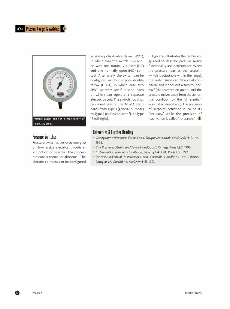
Pressure SwitchesPressure switches serve to energizeor de-energize electrical circuits asa function of whether the processpressure is normal or abnormal. Theelectric contacts can be configured
as single pole double throw (SPDT),in which case the switch is provid-ed with one normally closed (NC)and one normally open (NO) con-tact. Alternately, the switch can beconfigured as double pole doublethrow (DPDT), in which case twoSPDT switches are furnished, eachof which can operate a separateelectric circuit. The switch housingscan meet any of the NEMA stan-dards from Type 1 (general purpose)to Type 7 (explosion proof), or Type12 (oil tight).
Figure 5-3 illustrates the terminolo-gy used to describe pressure switchfunctionality and performance. Whenthe pressure reaches the setpoint(which is adjustable within the range),the switch signals an “abnormal con-dition” and it does not return to “nor-mal” (the reactivation point) until thepressure moves away from the abnor-mal condition by the “differential”(also called dead-band). The precisionof setpoint actuation is called its“accuracy,” while the precision ofreactivation is called “tolerance.” T
5Pressure Gauges & Switches
50 Volume 3 TRANSACTIONS
References & Further Reading• Omegadyne®Pressure, Force, Load, Torque Databook, OMEGADYNE, Inc.,
1996.• The Pressure, Strain, and Force Handbook™, Omega Press LLC, 1996.• Instrument Engineers’ Handbook, Bela Liptak, CRC Press LLC, 1995. • Process/Industrial Instruments and Controls Handbook, 4th Edition,
Douglas M. Considine, McGraw-Hill, 1993.
Pressure gauges come in a wide variety of
ranges and units.
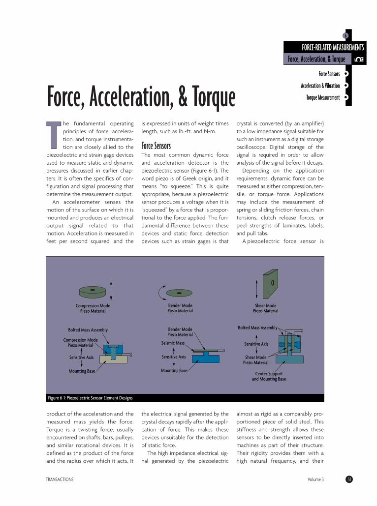
The fundamental operatingprinciples of force, accelera-tion, and torque instrumenta-tion are closely allied to the
piezoelectric and strain gage devicesused to measure static and dynamicpressures discussed in earlier chap-ters. It is often the specifics of con-figuration and signal processing thatdetermine the measurement output.
An accelerometer senses themotion of the surface on which it ismounted and produces an electricaloutput signal related to thatmotion. Acceleration is measured infeet per second squared, and the
product of the acceleration and themeasured mass yields the force.Torque is a twisting force, usuallyencountered on shafts, bars, pulleys,and similar rotational devices. It isdefined as the product of the forceand the radius over which it acts. It
is expressed in units of weight timeslength, such as lb.-ft. and N-m.
Force Sensors The most common dynamic forceand acceleration detector is thepiezoelectric sensor (Figure 6-1). Theword piezo is of Greek origin, and itmeans “to squeeze.” This is quiteappropriate, because a piezoelectricsensor produces a voltage when it is“squeezed” by a force that is propor-tional to the force applied. The fun-damental difference between thesedevices and static force detectiondevices such as strain gages is that
the electrical signal generated by thecrystal decays rapidly after the appli-cation of force. This makes thesedevices unsuitable for the detectionof static force.
The high impedance electrical sig-nal generated by the piezoelectric
crystal is converted (by an amplifier)to a low impedance signal suitable forsuch an instrument as a digital storageoscilloscope. Digital storage of thesignal is required in order to allowanalysis of the signal before it decays.
Depending on the applicationrequirements, dynamic force can bemeasured as either compression, ten-sile, or torque force. Applicationsmay include the measurement ofspring or sliding friction forces, chaintensions, clutch release forces, orpeel strengths of laminates, labels,and pull tabs.
A piezoelectric force sensor is
almost as rigid as a comparably pro-portioned piece of solid steel. Thisstiffness and strength allows thesesensors to be directly inserted intomachines as part of their structure.Their rigidity provides them with ahigh natural frequency, and their
TRANSACTIONS Volume 3 51
Force Sensors
Acceleration & Vibration
Torque Measurement
FORCE-RELATED MEASUREMENTS
6
Force, Acceleration, & Torque
TForce, Acceleration, & Torque
Compression Mode Piezo Material
Bender Mode Piezo Material
Shear Mode Piezo Material
Bender Mode Piezo Material
Seismic Mass
Mounting Base
Sensitive Axis
Bolted Mass Assembly
Shear Mode Piezo Material
Sensitive Axis
Center Support and Mounting Base
Bolted Mass Assembly
Compression Mode Piezo Material
Mounting Base
Sensitive Axis
Figure 6-1: Piezoelectric Sensor Element Designs
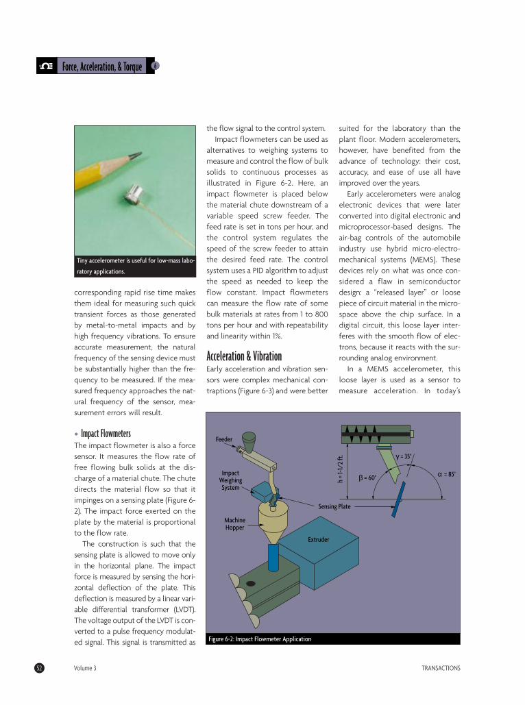
corresponding rapid rise time makesthem ideal for measuring such quicktransient forces as those generatedby metal-to-metal impacts and byhigh frequency vibrations. To ensureaccurate measurement, the naturalfrequency of the sensing device mustbe substantially higher than the fre-quency to be measured. If the mea-sured frequency approaches the nat-ural frequency of the sensor, mea-surement errors will result.
• Impact FlowmetersThe impact flowmeter is also a forcesensor. It measures the flow rate offree flowing bulk solids at the dis-charge of a material chute. The chutedirects the material flow so that itimpinges on a sensing plate (Figure 6-2). The impact force exerted on theplate by the material is proportionalto the flow rate.
The construction is such that thesensing plate is allowed to move onlyin the horizontal plane. The impactforce is measured by sensing the hori-zontal deflection of the plate. Thisdeflection is measured by a linear vari-able differential transformer (LVDT).The voltage output of the LVDT is con-verted to a pulse frequency modulat-ed signal. This signal is transmitted as
the flow signal to the control system.Impact flowmeters can be used as
alternatives to weighing systems tomeasure and control the flow of bulksolids to continuous processes asillustrated in Figure 6-2. Here, animpact flowmeter is placed belowthe material chute downstream of avariable speed screw feeder. Thefeed rate is set in tons per hour, andthe control system regulates thespeed of the screw feeder to attainthe desired feed rate. The controlsystem uses a PID algorithm to adjustthe speed as needed to keep theflow constant. Impact flowmeterscan measure the flow rate of somebulk materials at rates from 1 to 800tons per hour and with repeatabilityand linearity within 1%.
Acceleration & VibrationEarly acceleration and vibration sen-sors were complex mechanical con-traptions (Figure 6-3) and were better
suited for the laboratory than theplant floor. Modern accelerometers,however, have benefited from theadvance of technology: their cost,accuracy, and ease of use all haveimproved over the years.
Early accelerometers were analogelectronic devices that were laterconverted into digital electronic andmicroprocessor-based designs. Theair-bag controls of the automobileindustry use hybrid micro-electro-mechanical systems (MEMS). Thesedevices rely on what was once con-sidered a flaw in semiconductordesign: a “released layer” or loosepiece of circuit material in the micro-space above the chip surface. In adigital circuit, this loose layer inter-feres with the smooth flow of elec-trons, because it reacts with the sur-rounding analog environment.
In a MEMS accelerometer, thisloose layer is used as a sensor tomeasure acceleration. In today’s
6Force, Acceleration, & Torque
52 Volume 3 TRANSACTIONS
Impact Weighing System
Feeder
Machine Hopper
Extruder
h =
1-1/2
ft.
β = 60°
γ = 35°
α = 85°
Sensing Plate
Figure 6-2: Impact Flowmeter Application
Tiny accelerometer is useful for low-mass labo-
ratory applications.
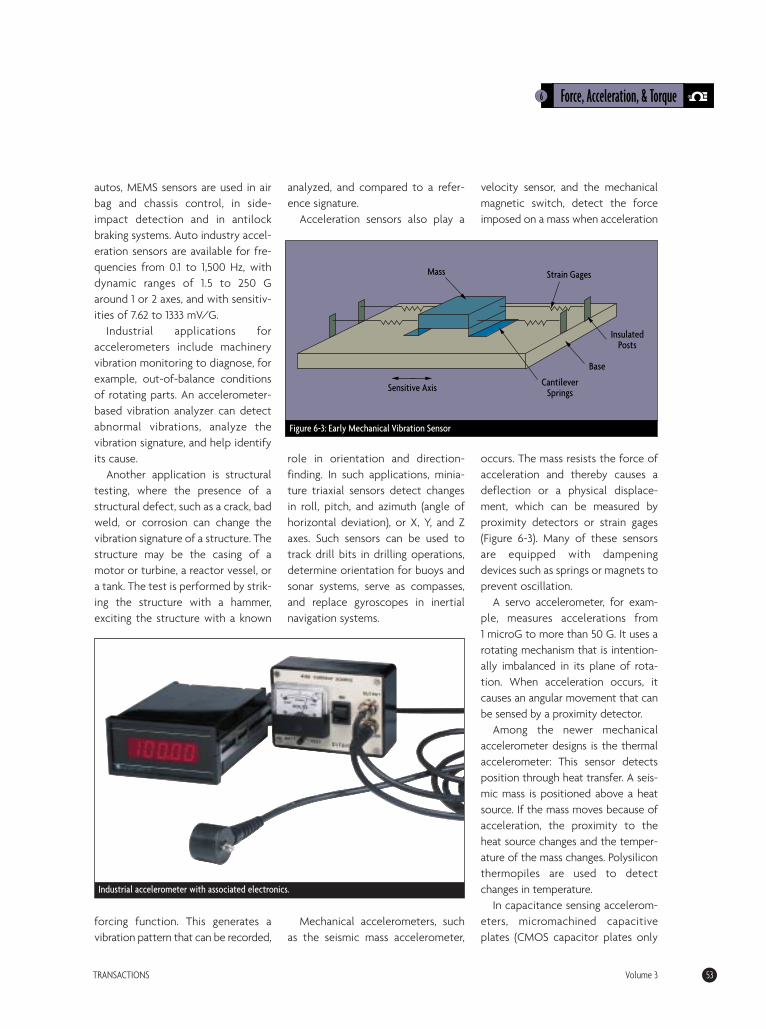
autos, MEMS sensors are used in airbag and chassis control, in side-impact detection and in antilockbraking systems. Auto industry accel-eration sensors are available for fre-quencies from 0.1 to 1,500 Hz, withdynamic ranges of 1.5 to 250 Garound 1 or 2 axes, and with sensitiv-ities of 7.62 to 1333 mV/G.
Industrial applications foraccelerometers include machineryvibration monitoring to diagnose, forexample, out-of-balance conditionsof rotating parts. An accelerometer-based vibration analyzer can detectabnormal vibrations, analyze thevibration signature, and help identifyits cause.
Another application is structuraltesting, where the presence of astructural defect, such as a crack, badweld, or corrosion can change thevibration signature of a structure. Thestructure may be the casing of amotor or turbine, a reactor vessel, ora tank. The test is performed by strik-ing the structure with a hammer,exciting the structure with a known
forcing function. This generates avibration pattern that can be recorded,
analyzed, and compared to a refer-ence signature.
Acceleration sensors also play a
role in orientation and direction-finding. In such applications, minia-ture triaxial sensors detect changesin roll, pitch, and azimuth (angle ofhorizontal deviation), or X, Y, and Zaxes. Such sensors can be used totrack drill bits in drilling operations,determine orientation for buoys andsonar systems, serve as compasses,and replace gyroscopes in inertialnavigation systems.
Mechanical accelerometers, suchas the seismic mass accelerometer,
velocity sensor, and the mechanicalmagnetic switch, detect the forceimposed on a mass when acceleration
occurs. The mass resists the force ofacceleration and thereby causes adeflection or a physical displace-ment, which can be measured byproximity detectors or strain gages(Figure 6-3). Many of these sensorsare equipped with dampeningdevices such as springs or magnets toprevent oscillation.
A servo accelerometer, for exam-ple, measures accelerations from1 microG to more than 50 G. It uses arotating mechanism that is intention-ally imbalanced in its plane of rota-tion. When acceleration occurs, itcauses an angular movement that canbe sensed by a proximity detector.
Among the newer mechanicalaccelerometer designs is the thermalaccelerometer: This sensor detectsposition through heat transfer. A seis-mic mass is positioned above a heatsource. If the mass moves because ofacceleration, the proximity to theheat source changes and the temper-ature of the mass changes. Polysiliconthermopiles are used to detectchanges in temperature.
In capacitance sensing accelerom-eters, micromachined capacitiveplates (CMOS capacitor plates only
6 Force, Acceleration, & Torque
TRANSACTIONS Volume 3 53
Mass Strain Gages
Insulated Posts
Base
Cantilever SpringsSensitive Axis
Figure 6-3: Early Mechanical Vibration Sensor
Industrial accelerometer with associated electronics.
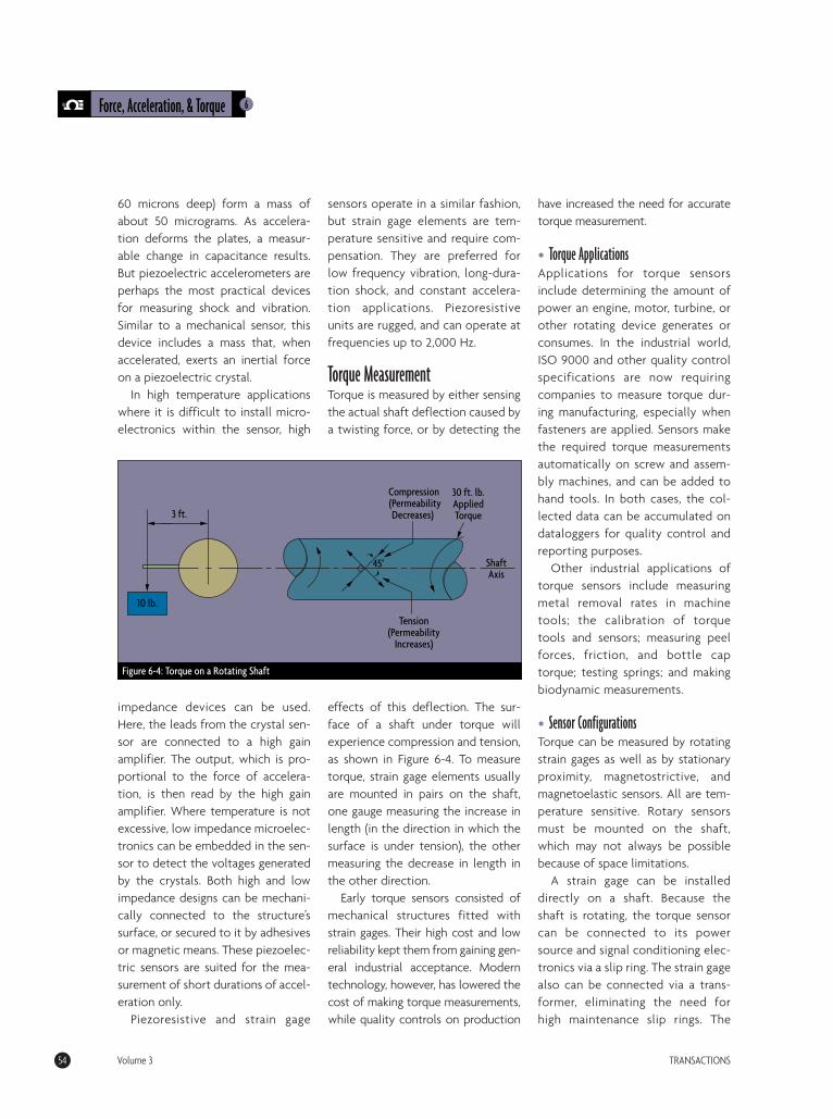
60 microns deep) form a mass ofabout 50 micrograms. As accelera-tion deforms the plates, a measur-able change in capacitance results.But piezoelectric accelerometers areperhaps the most practical devicesfor measuring shock and vibration.Similar to a mechanical sensor, thisdevice includes a mass that, whenaccelerated, exerts an inertial forceon a piezoelectric crystal.
In high temperature applicationswhere it is difficult to install micro-electronics within the sensor, high
impedance devices can be used.Here, the leads from the crystal sen-sor are connected to a high gainamplifier. The output, which is pro-portional to the force of accelera-tion, is then read by the high gainamplifier. Where temperature is notexcessive, low impedance microelec-tronics can be embedded in the sen-sor to detect the voltages generatedby the crystals. Both high and lowimpedance designs can be mechani-cally connected to the structure’ssurface, or secured to it by adhesivesor magnetic means. These piezoelec-tric sensors are suited for the mea-surement of short durations of accel-eration only.
Piezoresistive and strain gage
sensors operate in a similar fashion,but strain gage elements are tem-perature sensitive and require com-pensation. They are preferred forlow frequency vibration, long-dura-tion shock, and constant accelera-tion applications. Piezoresistiveunits are rugged, and can operate atfrequencies up to 2,000 Hz.
Torque MeasurementTorque is measured by either sensingthe actual shaft deflection caused bya twisting force, or by detecting the
effects of this deflection. The sur-face of a shaft under torque willexperience compression and tension,as shown in Figure 6-4. To measuretorque, strain gage elements usuallyare mounted in pairs on the shaft,one gauge measuring the increase inlength (in the direction in which thesurface is under tension), the othermeasuring the decrease in length inthe other direction.
Early torque sensors consisted ofmechanical structures fitted withstrain gages. Their high cost and lowreliability kept them from gaining gen-eral industrial acceptance. Moderntechnology, however, has lowered thecost of making torque measurements,while quality controls on production
have increased the need for accuratetorque measurement.
• Torque ApplicationsApplications for torque sensorsinclude determining the amount ofpower an engine, motor, turbine, orother rotating device generates orconsumes. In the industrial world,ISO 9000 and other quality controlspecifications are now requiringcompanies to measure torque dur-ing manufacturing, especially whenfasteners are applied. Sensors makethe required torque measurementsautomatically on screw and assem-bly machines, and can be added tohand tools. In both cases, the col-lected data can be accumulated ondataloggers for quality control andreporting purposes.
Other industrial applications oftorque sensors include measuringmetal removal rates in machinetools; the calibration of torquetools and sensors; measuring peelforces, friction, and bottle captorque; testing springs; and makingbiodynamic measurements.
• Sensor ConfigurationsTorque can be measured by rotatingstrain gages as well as by stationaryproximity, magnetostrictive, andmagnetoelastic sensors. All are tem-perature sensitive. Rotary sensorsmust be mounted on the shaft,which may not always be possiblebecause of space limitations.
A strain gage can be installeddirectly on a shaft. Because theshaft is rotating, the torque sensorcan be connected to its powersource and signal conditioning elec-tronics via a slip ring. The strain gagealso can be connected via a trans-former, eliminating the need forhigh maintenance slip rings. The
6Force, Acceleration, & Torque
54 Volume 3 TRANSACTIONS
3 ft.
Compression (Permeability
Decreases)
30 ft. lb. Applied Torque
Shaft Axis
Tension (Permeability
Increases)
10 lb.
45°
Figure 6-4: Torque on a Rotating Shaft

excitation voltage for the straingage is inductively coupled, and thestrain gage output is converted to amodulated pulse frequency (Figure6-5). Maximum speed of such anarrangement is 15,000 rpm.
Strain gages also can be mountedon stationary support members or onthe housing itself. These “reaction”sensors measure the torque that istransferred by the shaft to therestraining elements. The resultantreading is not completely accurate, asit disregards the inertia of the motor.
Strain gages used for torque mea-surements include foil, diffusedsemiconductor, and thin film types.These can be attached directly tothe shaft by soldering or adhesives. Ifthe centrifugal forces are not large—and an out-of-balance load can betolerated—the associated electron-ics, including battery, amplifier, andradio frequency transmitter all can
be strapped to the shaft.Proximity and displacement sensors
also can detect torque by measuringthe angular displacement between ashaft’s two ends. By fixing two identi-cal toothed wheels to the shaft atsome distance apart, the angular dis-placement caused by the torque canbe measured. Proximity sensors or
photocells located at each toothedwheel produce output voltages
whose phase difference increases asthe torque twists the shaft.
Another approach is to aim a sin-gle photocell through both sets oftoothed wheels. As torque risesand causes one wheel to overlapthe other, the amount of lightreaching the photocell is reduced.Displacements caused by torque canalso be detected by other optical,inductive, capacitive, and potentio-metric sensors. For example, a capaci-tance-type torque sensor can measurethe change in capacitance that occurswhen torque causes the gap betweentwo capacitance plates to vary.
The ability of a shaft material toconcentrate magnetic flux—mag-netic permeability—also varies withtorque and can be measured using amagnetostrictive sensor. When theshaft has no loading, its permeabili-ty is uniform. Under torsion, perme-ability and the number of flux linesincrease in proportion to torque.This type of sensor can be mountedto the side of the shaft using twoprimary and two secondary wind-ings. Alternatively, it can bearranged with many primary andsecondary windings on a ring
6 Force, Acceleration, & Torque
TRANSACTIONS Volume 3 55
Oscillator (Supply)
Amplifier Demodulator
Output Signal
Bridge Excitation Strain
Elements
Torque Bridge
Bridge Output
STATIONARY PORTION ROTATING PORTION
Figure 6-5: Inductive Coupling of Torque Sensors
Reaction torque cell with flange mounts.
around the shaft.A magnetoelastic torque sensor
detects changes in permeability bymeasuring changes in its own mag-netic field. One magnetoelastic sen-sor is constructed as a thin ring ofsteel tightly coupled to a stainlesssteel shaft. This assembly acts as apermanent magnet whose magneticfield is proportional to the torqueapplied to the shaft. The shaft isconnected between a drive motorand the driven device, such as ascrew machine. A magnetometerconverts the generated magneticfield into an electrical output signalthat is proportional to the torquebeing applied. T
6Force, Acceleration, & Torque
56 Volume 3 TRANSACTIONS
References & Further Reading• Omegadyne®Pressure, Force, Load, Torque Databook, OMEGADYNE, Inc.,
1996.• The Pressure, Strain, and Force Handbook™, Omega Press LLC, 1996.• Industrial Control Handbook, E. A. Parr, Butterworth, 1995.• Instrument Engineers’ Handbook, Bela Liptak, CRC Press LLC, 1995.• Instrumentation Reference Book, 2nd Edition, B.E. Noltingk, Butterworth-
Heinemann, 1995.• “Overcoming the High Cost of Torque Sensing in Industrial Applications,”
Darrell Williams, Eaton Corp., 1998.• Process/Industrial Instruments and Controls Handbook, 4th Edition,
Douglas M. Considine, McGraw-Hill, 1993.• Sensor and Analyzer Handbook, H.N. Norton, Prentice Hall, 1982.• “Sensors: The Next Wave of Infotech Innovation,” Paul Saffo, Institute for
the Future, 1998.• Van Nostrand’s Scientific Encyclopedia, Douglas M. Considine and Glenn
D. Considine, Van Nostrand, 1997.• Vibration Analysis for Electronic Equipment, 2nd Edition, Dave S.
Steinberg, Wiley, 1988.
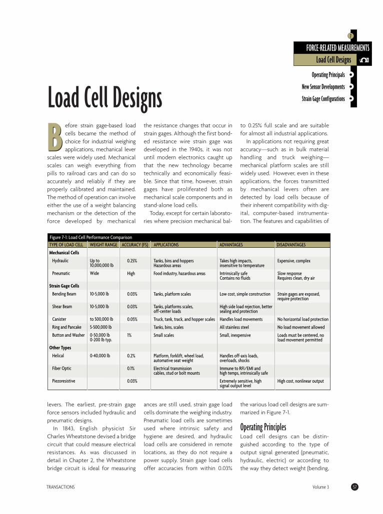
Before strain gage-based loadcells became the method ofchoice for industrial weighingapplications, mechanical lever
scales were widely used. Mechanicalscales can weigh everything frompills to railroad cars and can do soaccurately and reliably if they areproperly calibrated and maintained.The method of operation can involveeither the use of a weight balancingmechanism or the detection of theforce developed by mechanical
levers. The earliest, pre-strain gageforce sensors included hydraulic andpneumatic designs.
In 1843, English physicist SirCharles Wheatstone devised a bridgecircuit that could measure electricalresistances. As was discussed indetail in Chapter 2, the Wheatstonebridge circuit is ideal for measuring
the resistance changes that occur instrain gages. Although the first bond-ed resistance wire strain gage wasdeveloped in the 1940s, it was notuntil modern electronics caught upthat the new technology becametechnically and economically feasi-ble. Since that time, however, straingages have proliferated both asmechanical scale components and instand-alone load cells.
Today, except for certain laborato-ries where precision mechanical bal-
ances are still used, strain gage loadcells dominate the weighing industry.Pneumatic load cells are sometimesused where intrinsic safety andhygiene are desired, and hydraulicload cells are considered in remotelocations, as they do not require apower supply. Strain gage load cellsoffer accuracies from within 0.03%
to 0.25% full scale and are suitablefor almost all industrial applications.
In applications not requiring greataccuracy—such as in bulk materialhandling and truck weighing—mechanical platform scales are stillwidely used. However, even in theseapplications, the forces transmittedby mechanical levers often aredetected by load cells because oftheir inherent compatibility with dig-ital, computer-based instrumenta-tion. The features and capabilities of
the various load cell designs are sum-marized in Figure 7-1.
Operating PrinciplesLoad cell designs can be distin-guished according to the type ofoutput signal generated (pneumatic,hydraulic, electric) or according tothe way they detect weight (bending,
TRANSACTIONS Volume 3 57
B
Mechanical Cells
Hydraulic
Pneumatic
Strain Gage Cells
Bending Beam
Shear Beam
Canister
Ring and Pancake
Button and Washer
Other Types
Helical
Fiber Optic
Piezoresistive
TYPE OF LOAD CELL WEIGHT RANGE ACCURACY (FS) APPLICATIONS ADVANTAGES DISADVANTAGES
Up to 10,000,000 lb
Wide
10-5,000 lb
10-5,000 lb
to 500,000 lb
5-500,000 lb
0-50,000 lb 0-200 lb typ.
0-40,000 lb
Figure 7-1: Load Cell Performance Comparison
0.25%
High
0.03%
0.03%
0.05%
1%
0.2%
0.1%
0.03%
Tanks, bins and hoppers Hazardous areas
Food industry, hazardous areas
Tanks, platform scales
Tanks, platforms scales, off-center loads
Truck, tank, track, and hopper scales
Tanks, bins, scales
Small scales
Platform, forklift, wheel load, automative seat weight
Electrical transmission cables, stud or bolt mounts
Takes high impacts, insensitive to temperature
Intrinsically safe Contains no fluids
Low cost, simple construction
High side load rejection, better sealing and protection
Handles load movements
All stainless steel
Small, inexpensive
Handles off-axis loads, overloads, shocks
Immune to RFI/EMI and high temps, intrinsically safe
Extremely sensitive, high signal output level
Expensive, complex
Slow response Requires clean, dry air
Strain gages are exposed, require protection
No horizontal load protection
No load movement allowed
Loads must be centered, no load movement permitted
High cost, nonlinear output
Operating Principals
New Sensor Developments
Strain Gage Configurations
FORCE-RELATED MEASUREMENTS
7
Load Cell Designs
Load Cell Designs
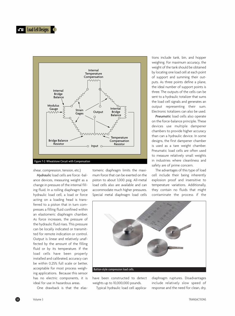
shear, compression, tension, etc.)Hydraulic load cells are force -bal-
ance devices, measuring weight as achange in pressure of the internal fill-ing fluid. In a rolling diaphragm typehydraulic load cell, a load or forceacting on a loading head is trans-ferred to a piston that in turn com-presses a filling fluid confined withinan elastomeric diaphragm chamber.As force increases, the pressure ofthe hydraulic fluid rises. This pressurecan be locally indicated or transmit-ted for remote indication or control.Output is linear and relatively unaf-fected by the amount of the fillingfluid or by its temperature. If theload cells have been properlyinstalled and calibrated, accuracy canbe within 0.25% full scale or better,acceptable for most process weigh-ing applications. Because this sensorhas no electric components, it isideal for use in hazardous areas.
One drawback is that the elas-
tomeric diaphragm limits the maxi-mum force that can be exerted on thepiston to about 1,000 psig. All-metalload cells also are available and canaccommodate much higher pressures.Special metal diaphragm load cells
have been constructed to detectweights up to 10,000,000 pounds.
Typical hydraulic load cell applica-
tions include tank, bin, and hopperweighing. For maximum accuracy, theweight of the tank should be obtainedby locating one load cell at each pointof support and summing their out-puts. As three points define a plane,the ideal number of support points isthree. The outputs of the cells can besent to a hydraulic totalizer that sumsthe load cell signals and generates anoutput representing their sum.Electronic totalizers can also be used.
Pneumatic load cells also operateon the force-balance principle. Thesedevices use multiple dampenerchambers to provide higher accuracythan can a hydraulic device. In somedesigns, the first dampener chamberis used as a tare weight chamber.Pneumatic load cells are often usedto measure relatively small weightsin industries where cleanliness andsafety are of prime concern.
The advantages of this type of loadcell include their being inherentlyexplosion proof and insensitive totemperature variations. Additionally,they contain no fluids that mightcontaminate the process if the
diaphragm ruptures. Disadvantagesinclude relatively slow speed ofresponse and the need for clean, dry,
7Load Cell Designs
58 Volume 3 TRANSACTIONS
Bridge Balance Resistor
Modulus Gauge Strain
Gages Output
Input
Internal Temperature
Compensation
Internal Bridge
Balance
Temperature Compensation
Resistor
Internal Bridge Balance
Figure 7-2: Wheatstone Circuit with Compensation
Button-style compression load cells.
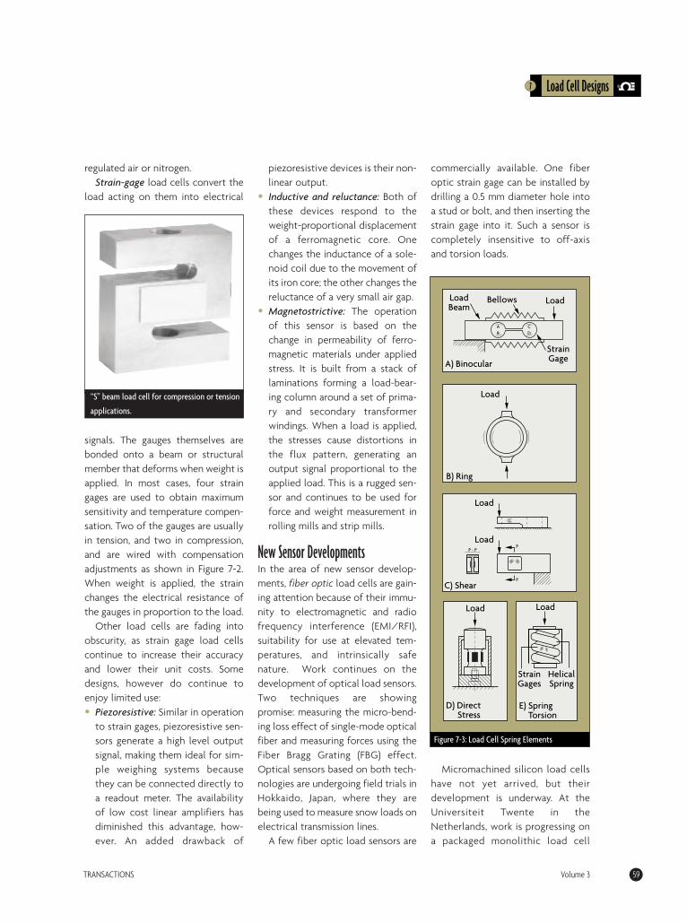
regulated air or nitrogen.Strain-gage load cells convert the
load acting on them into electrical
signals. The gauges themselves arebonded onto a beam or structuralmember that deforms when weight isapplied. In most cases, four straingages are used to obtain maximumsensitivity and temperature compen-sation. Two of the gauges are usuallyin tension, and two in compression,and are wired with compensationadjustments as shown in Figure 7-2.When weight is applied, the strainchanges the electrical resistance ofthe gauges in proportion to the load.
Other load cells are fading intoobscurity, as strain gage load cellscontinue to increase their accuracyand lower their unit costs. Somedesigns, however do continue toenjoy limited use:• Piezoresistive: Similar in operation
to strain gages, piezoresistive sen-sors generate a high level outputsignal, making them ideal for sim-ple weighing systems becausethey can be connected directly toa readout meter. The availabilityof low cost linear amplifiers hasdiminished this advantage, how-ever. An added drawback of
piezoresistive devices is their non-linear output.
• Inductive and reluctance: Both ofthese devices respond to theweight-proportional displacementof a ferromagnetic core. Onechanges the inductance of a sole-noid coil due to the movement ofits iron core; the other changes thereluctance of a very small air gap.
• Magnetostrictive: The operationof this sensor is based on thechange in permeability of ferro-magnetic materials under appliedstress. It is built from a stack oflaminations forming a load-bear-ing column around a set of prima-ry and secondary transformerwindings. When a load is applied,the stresses cause distortions inthe flux pattern, generating anoutput signal proportional to theapplied load. This is a rugged sen-sor and continues to be used forforce and weight measurement inrolling mills and strip mills.
New Sensor DevelopmentsIn the area of new sensor develop-ments, fiber optic load cells are gain-ing attention because of their immu-nity to electromagnetic and radiofrequency interference (EMI/RFI),suitability for use at elevated tem-peratures, and intrinsically safenature. Work continues on thedevelopment of optical load sensors.Two techniques are showingpromise: measuring the micro-bend-ing loss effect of single-mode opticalfiber and measuring forces using theFiber Bragg Grating (FBG) effect.Optical sensors based on both tech-nologies are undergoing field trials inHokkaido, Japan, where they arebeing used to measure snow loads onelectrical transmission lines.
A few fiber optic load sensors are
commercially available. One fiberoptic strain gage can be installed bydrilling a 0.5 mm diameter hole intoa stud or bolt, and then inserting thestrain gage into it. Such a sensor iscompletely insensitive to off-axisand torsion loads.
Micromachined silicon load cellshave not yet arrived, but theirdevelopment is underway. At theUniversiteit Twente in theNetherlands, work is progressing ona packaged monolithic load cell
7 Load Cell Designs
TRANSACTIONS Volume 3 59
Figure 7-3: Load Cell Spring Elements
AB
CD
Load Beam
Bellows Load
Strain Gage
Load
A) Binocular
B) Ring
C) Shear
D) Direct Stress
E) Spring Torsion
PP - P
P
Load
Load
Load Load
Strain Gages
Helical Spring
“S” beam load cell for compression or tension
applications.
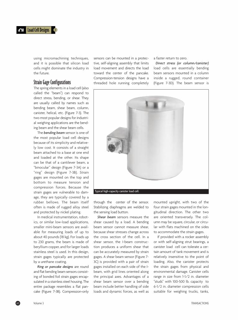
using micromachining techniques,and it is possible that silicon loadcells might dominate the industry inthe future.
Strain Gage ConfigurationsThe spring elements in a load cell (alsocalled the “beam”) can respond todirect stress, bending, or shear. Theyare usually called by names such asbending beam, shear beam, column,canister, helical, etc. (Figure 7-3). Thetwo most popular designs for industri-al weighing applications are the bend-ing beam and the shear beam cells.
The bending beam sensor is one ofthe most popular load cell designsbecause of its simplicity and relative-ly low cost. It consists of a straightbeam attached to a base at one endand loaded at the other. Its shapecan be that of a cantilever beam, a“binocular” design (Figure 7-3A) or a“ring” design (Figure 7-3B). Straingages are mounted on the top andbottom to measure tension andcompression forces. Because thestrain gages are vulnerable to dam-age, they are typically covered by arubber bellows. The beam itselfoften is made of rugged alloy steeland protected by nickel plating.
In medical instrumentation, robot-ics, or similar low-load applications,smaller mini-beam sensors are avail-able for measuring loads of up toabout 40 pounds (18 kg). For loads upto 230 grams, the beam is made ofberyllium copper, and for larger loadsstainless steel is used. In this design,strain gages typically are protectedby a urethane coating.
Ring or pancake designs are roundand flat bending beam sensors consist-ing of bonded foil strain gages encap-sulated in a stainless steel housing. Theentire package resembles a flat pan-cake (Figure 7-3B). Compression-only
sensors can be mounted in a protec-tive, self-aligning assembly that limitsload movement and directs the loadtoward the center of the pancake.Compression-tension designs have athreaded hole running completely
through the center of the sensor.Stabilizing diaphragms are welded tothe sensing load button.
Shear beam sensors measure theshear caused by a load. A bendingbeam sensor cannot measure shear,because shear stresses change acrossthe cross section of the cell. In ashear sensor, the I-beam construc-tion produces a uniform shear thatcan be accurately measured by straingages. A shear beam sensor (Figure 7-3C) is provided with a pair of straingages installed on each side of the I-beam, with grid lines oriented alongthe principal axes. Advantages of ashear beam sensor over a bendingbeam include better handling of sideloads and dynamic forces, as well as
a faster return to zero. Direct stress (or column/canister)
load cells are essentially bendingbeam sensors mounted in a columninside a rugged, round container(Figure 7-3D). The beam sensor is
mounted upright, with two of thefour strain gages mounted in the lon-gitudinal direction. The other twoare oriented transversely. The col-umn may be square, circular, or circu-lar with flats machined on the sidesto accommodate the strain gages.
If provided with a rocker assemblyor with self-aligning strut bearings, acanister load cell can tolerate a cer-tain amount of tank movement and isrelatively insensitive to the point ofloading. Also, the canister protectsthe strain gages from physical andenvironmental damage. Canister cellsrange in size from 1-1/2 in. diameter“studs” with 100-500 lb. capacity to6-1/2 in. diameter compression cellssuitable for weighing trucks, tanks,
7Load Cell Designs
60 Volume 3 TRANSACTIONS
Typical high-capacity canister load cell.
and hoppers up to 500,000 lb. Helical load cells are better able
to handle off-axis loading than arecanister-type compression cells(Figure 7-3E). The operation of ahelical load cell is based on that ofa spring. A spring balances a loadforce by its own torsional moment.The torsional reaction travels fromthe top of the helix to the bottom.By measuring this torsional momentwith strain gages mounted on thespring, a helical load cell can pro-vide reasonably accurate load mea-surement without the need forexpensive mounting structures.Forces caused by asymmetrical oroff-axis loading have little effect onthe spring, and the strain gage sen-sors can measure both tension andcompression forces.
A helical load cell can be mountedon rough surfaces, even where theupper and lower surfaces are not par-allel, and total error can still remainwithin 0.5%. The helical load cell alsois resistant to shock and overload (itcan handle a thousandfold overload),
making it ideal for force or load mea-surements on vehicle axles, seats, or inforklift applications.
Button and flat washer bondedstrain gage load cells are available insizes from 1/4 to 1-1/2 in. diameter.The smallest sensors are availableonly in compression styles, but someof the larger cells have threadedholes for also measuring tension.While most of the tiny sensors han-dle up to about 200 lb., some are
capable of measuring up to 50,000 lb.Because these little cells have no fix-tures or flexures, off-axis loading andshifting loads cannot be tolerated.
On the other hand, button andflat washer load cells are extremelyconvenient and easy to use. Even thesmallest sensor is built of stainlesssteel, has a built in, full four-armWheatstone bridge, and can mea-sure up to 200 lb. at temperatures upto 1500°F. T
7 Load Cell Designs
TRANSACTIONS Volume 3 61
References & Further Reading• Omegadyne®Pressure, Force, Load, Torque Databook, OMEGADYNE, Inc.,
1996.• The Pressure, Strain, and Force Handbook™, Omega Press LLC, 1996.• Elements of Electronic Instrumentation and Measurements, 3rd Edition,
Joseph J. Carr, Prentice Hall, 1996.• Industrial Control Handbook, E.A. Parr, Butterworth-Heinemann, 1995.• Instrument Engineers’ Handbook, Bela Liptak, CRC Press LLC, 1995. • Process/Industrial Instruments and Controls Handbook, 4th Edition,
Douglas M. Considine, McGraw-Hill, 1993.• Van Nostrand’s Scientific Encyclopedia, Douglas M. Considine and Glenn
D. Considine, Van Nostrand, 1997.• Weighing and Force Measurement in the ‘90s, T. Kemeny, IMEKO TC
Series, 1991.
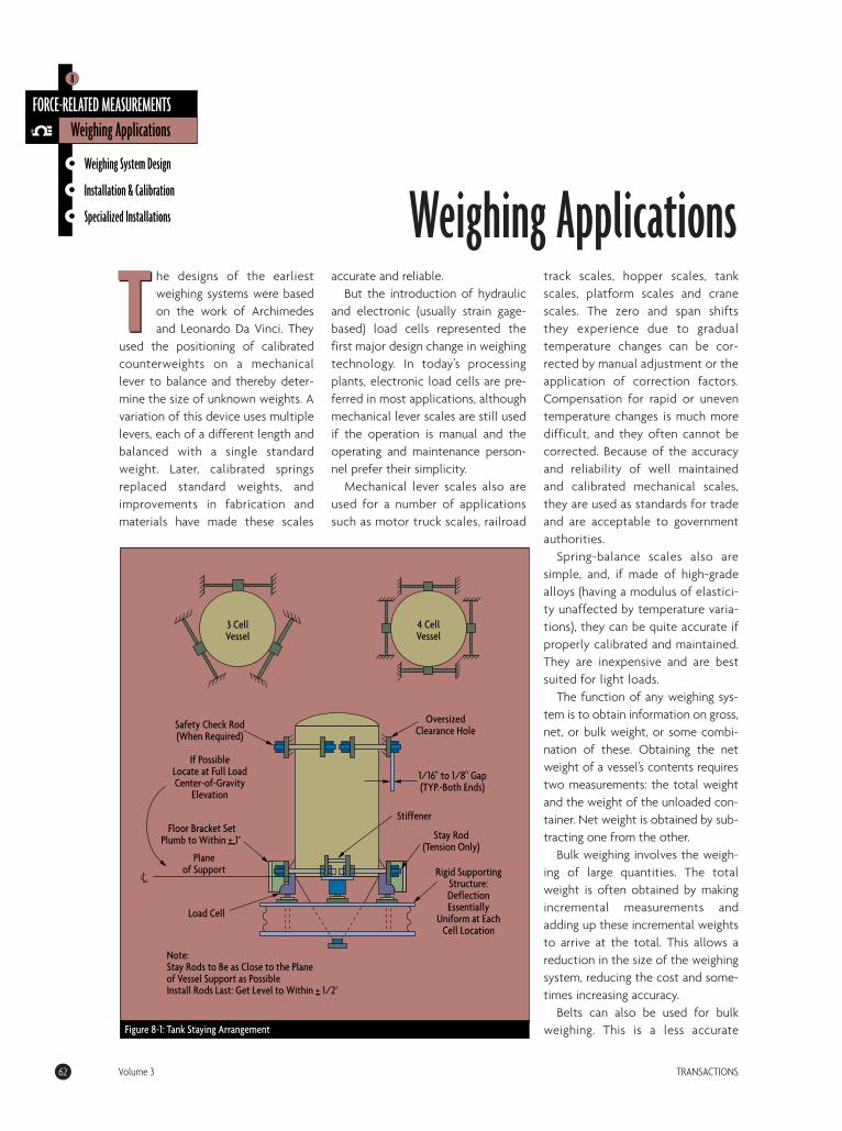
The designs of the earliestweighing systems were basedon the work of Archimedesand Leonardo Da Vinci. They
used the positioning of calibratedcounterweights on a mechanicallever to balance and thereby deter-mine the size of unknown weights. Avariation of this device uses multiplelevers, each of a different length andbalanced with a single standardweight. Later, calibrated springsreplaced standard weights, andimprovements in fabrication andmaterials have made these scales
accurate and reliable. But the introduction of hydraulic
and electronic (usually strain gage-based) load cells represented thefirst major design change in weighingtechnology. In today’s processingplants, electronic load cells are pre-ferred in most applications, althoughmechanical lever scales are still usedif the operation is manual and theoperating and maintenance person-nel prefer their simplicity.
Mechanical lever scales also areused for a number of applicationssuch as motor truck scales, railroad
track scales, hopper scales, tankscales, platform scales and cranescales. The zero and span shiftsthey experience due to gradualtemperature changes can be cor-rected by manual adjustment or theapplication of correction factors.Compensation for rapid or uneventemperature changes is much moredifficult, and they often cannot becorrected. Because of the accuracyand reliability of well maintainedand calibrated mechanical scales,they are used as standards for tradeand are acceptable to governmentauthorities.
Spring-balance scales also aresimple, and, if made of high-gradealloys (having a modulus of elastici-ty unaffected by temperature varia-tions), they can be quite accurate ifproperly calibrated and maintained.They are inexpensive and are bestsuited for light loads.
The function of any weighing sys-tem is to obtain information on gross,net, or bulk weight, or some combi-nation of these. Obtaining the netweight of a vessel’s contents requirestwo measurements: the total weightand the weight of the unloaded con-tainer. Net weight is obtained by sub-tracting one from the other.
Bulk weighing involves the weigh-ing of large quantities. The totalweight is often obtained by makingincremental measurements andadding up these incremental weightsto arrive at the total. This allows areduction in the size of the weighingsystem, reducing the cost and some-times increasing accuracy.
Belts can also be used for bulkweighing. This is a less accurate
62 Volume 3 TRANSACTIONS
Weighing System Design
Installation & Calibration
Specialized Installations
FORCE-RELATED MEASUREMENTSWeighing Applications
8
TWeighing Applications
3 Cell Vessel
4 Cell Vessel
Safety Check Rod (When Required)
If Possible
Locate at Full Load Center-of-Gravity
Elevation
Oversized Clearance Hole
Stiffener
Stay Rod (Tension Only)
Rigid Supporting Structure: Deflection Essentially
Uniform at Each Cell Location
Load Cell
Floor Bracket Set Plumb to Within + 1°
Plane of Support
1/16" to 1/8" Gap (TYP.-Both Ends)
Note: Stay Rods to Be as Close to the Plane of Vessel Support as Possible Install Rods Last: Get Level to Within + 1/2°
Figure 8-1: Tank Staying Arrangement
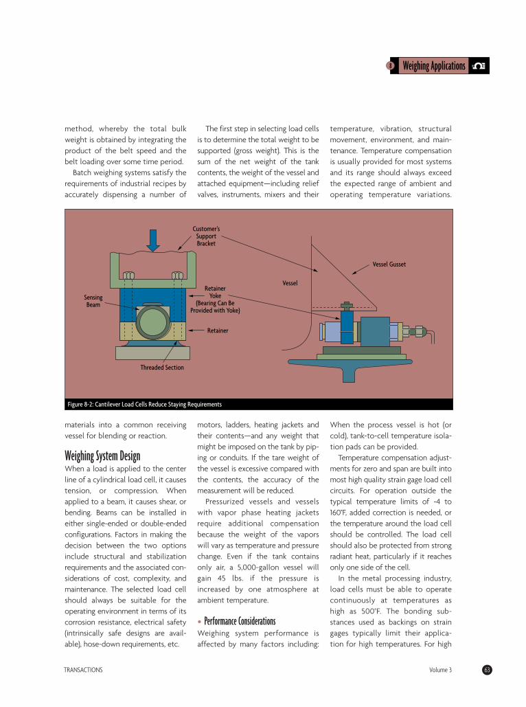
method, whereby the total bulkweight is obtained by integrating theproduct of the belt speed and thebelt loading over some time period.
Batch weighing systems satisfy therequirements of industrial recipes byaccurately dispensing a number of
materials into a common receivingvessel for blending or reaction.
Weighing System DesignWhen a load is applied to the centerline of a cylindrical load cell, it causestension, or compression. Whenapplied to a beam, it causes shear, orbending. Beams can be installed ineither single-ended or double-endedconfigurations. Factors in making thedecision between the two optionsinclude structural and stabilizationrequirements and the associated con-siderations of cost, complexity, andmaintenance. The selected load cellshould always be suitable for theoperating environment in terms of itscorrosion resistance, electrical safety(intrinsically safe designs are avail-able), hose-down requirements, etc.
The first step in selecting load cellsis to determine the total weight to besupported (gross weight). This is thesum of the net weight of the tankcontents, the weight of the vessel andattached equipment—including reliefvalves, instruments, mixers and their
motors, ladders, heating jackets andtheir contents—and any weight thatmight be imposed on the tank by pip-ing or conduits. If the tare weight ofthe vessel is excessive compared withthe contents, the accuracy of themeasurement will be reduced.
Pressurized vessels and vesselswith vapor phase heating jacketsrequire additional compensationbecause the weight of the vaporswill vary as temperature and pressurechange. Even if the tank containsonly air, a 5,000-gallon vessel willgain 45 lbs. if the pressure isincreased by one atmosphere atambient temperature.
• Performance Considerations Weighing system performance isaffected by many factors including:
temperature, vibration, structuralmovement, environment, and main-tenance. Temperature compensationis usually provided for most systemsand its range should always exceedthe expected range of ambient andoperating temperature variations.
When the process vessel is hot (orcold), tank-to-cell temperature isola-tion pads can be provided.
Temperature compensation adjust-ments for zero and span are built intomost high quality strain gage load cellcircuits. For operation outside thetypical temperature limits of -4 to160°F, added correction is needed, orthe temperature around the load cellshould be controlled. The load cellshould also be protected from strongradiant heat, particularly if it reachesonly one side of the cell.
In the metal processing industry,load cells must be able to operatecontinuously at temperatures ashigh as 500°F. The bonding sub-stances used as backings on straingages typically limit their applica-tion for high temperatures. For high
8 Weighing Applications
TRANSACTIONS Volume 3 63
Customer's Support Bracket
Sensing Beam
Retainer Yoke
(Bearing Can Be Provided with Yoke)
Retainer
Vessel
Vessel Gusset
Threaded Section
Figure 8-2: Cantilever Load Cells Reduce Staying Requirements

temperature applications, strainsensing wire alloys can be installedwith inorganic (ceramic) bondingcement. Alternatively, a flame spraytechnique can be used, where moltenaluminum oxide is sprayed on thestrain sensing grid to hold it in place.Such installations can tolerate short-term operations up to 1000°F.
Vibration influences can be mini-mized by isolating the weighing systemsupports from structures or concretefoundations that support motors orother vibrating equipment or areaffected by nearby vehicular traffic.Vibration absorption pads are availableto isolate the load cells from the vibra-tion of the tank, but performance willbe best if isolation pads are used at thevibration source. Similarly, weighttransmitters can be provided with fil-tering for the removal of noise caused
by vibration, but it is best if vibrationdoes not exist in the first place. Duringweighing, it is desirable to stop all in-and outflows and to turn off allmotors and mixers that are attachedto the weighed tank, if at all possible.
In agitated vessels, baffle plates shouldbe added to reduce surging and gyra-tion of the contents.
The load cell environment is adynamic one and therefore requiresperiodic checking. This shouldinclude an attempt to keep thecell(s), cable, and associated junctionbox clear of debris, ice, or standingwater (or other liquids), and shieldedfrom heat, direct sunlight, and wind.Cells should also be protected fromlightning and electrical surges.Maintenance should include checkingthe load cell environment, structures,wiring and junction boxes (for mois-ture and to tighten terminals), adjust-ment of stay and check rods, and peri-odic calibration and checking to makesure that the load is balanced.
Load cells can withstand up to200% of their capacity in side loads.
If a vessel is bumped by a vehicle oris otherwise disturbed, the cellsshould be checked for damage andbe recalibrated. Maintenance relatedchecking should be performed withthe vessel both loaded and
unloaded, and at all possible ves-sel/structure temperatures.
• Vessel Support Structure The next step in the design process isthe selection of the required struc-tural supports for the tank. Tensionsupport can only be used to weighsmall vessels because of the limitedweight ranges of tension cells. In ten-sion-type installations, one to fourcells are used (usually one), while incompression-type installations usu-ally three or more are used. Whenaccuracy is not critical (0.5% fullscale or less) and the tank contains aliquid, costs can be reduced byreplacing load cells with dummycells or with flexure beams. Verticalround tanks are typically supportedoff three, while four are used forsquare or horizontal round vessels. Itis preferable that all load cells in thesystem be of the same capacity.
Vessels that are very large, haveunbalanced loads, contain hazardousmaterials, or are at risk of overturningmight use more cells. If wind shield-ing is not provided for the vessel, cellcapacity must be increased to alsoprovide for the uplift and down-thrust caused by the worst case ofwind-induced tipping.
Three cells are best for accurateweighing because three points definea plane and therefore the load willbe equalized naturally. Four or morecells require load adjustments. Theminimum load cell range (size) isobtained by dividing the grossweight by the number of supportpoints. One usually selects the nextstandard cell which exceeds the cal-culated requirement. Some applica-tion engineers will add a safety fac-tor of 25% to the gross weight beforemaking the above calculation. Otherswill also add a dynamic loading
8Weighing Applications
64 Volume 3 TRANSACTIONS
Figure 8-3: End-Loaded Shear-Beam Installation
Platform Main Side Rail
Load Cell Electrical Cable
Fitting Double Parallel Link Suspension
Direction of Traffic
Steel and Concrete Foundation Load Cell
SupportLink Suspension
Support
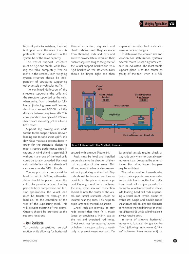
factor if, prior to weighing, the loadis dropped onto the scale. It also ispreferable that all load cells in thesystem be of the same capacity.
The vessel support structuremust be rigid and stable, while leav-ing the tank completely free tomove in the vertical. Each weighingsystem structure should be inde-pendent of structures supportingother vessels or vehicular traffic.
The combined deflection of thestructure supporting the cells andthe structure supported by the cells,when going from unloaded to fullyloaded (including vessel wall flexure),should not exceed 1/1,200th of thedistance between any two cells. Thiscorresponds to an angle of 0.5°. Someshear beam mounting yokes allow alittle more.
Support leg bowing also addstorque to the support beam. Unevenloading due to wind shear, uplift, anddownload must also be considered inorder for the structural design tomeet structure performance specifi-cations. A wind shield is essential, ifwithout it any one of the load cellscould be totally unloaded. For mostcells, wind effect without shields willcause errors under 0.1% full scale.
The support structure should belevel to within 1/8 in.; otherwise,shims should be placed under thecell(s) to provide a level loadingplane. In both compression and ten-sion applications, the vessel loadmust be transferred through theload cell to the centerline of theweb of the supporting steel. Thiswill prevent twisting of the beams.Gussets should be provided at thesupport locations.
• Vessel Stabilization To provide unrestricted verticalmotion while allowing for horizontal
thermal expansion, stay rods andcheck rods are used. They are madefrom threaded rods and nuts andserve to provide lateral restraint. Theirnuts are adjusted snug to the gusset ofthe vessel support bracket and to arigid bracket on the structure. Nutsshould be finger tight and then
secured with jam nuts (Figure 8-1).Rods must be level and installed
perpendicular to the direction of ther-mal expansion of the vessel. Thisallows unrestricted vertical movementwithout producing a side load. Stayrods should be installed as close aspossible to the plane of vessel sup-port. On long, round, horizontal tanks,the axial vessel stay rod connectionshould be near the center of the ves-sel, and lateral restraints should belocated near the ends. This helps toavoid large axial thermal expansion.
Check rods are identical to stayrods except that their fit is madeloose by providing a 1/8-in. gap atthe nut and oversized rod holes.Check rods may be mounted aboveor below the support plane or verti-cally to prevent vessel overturn. On
suspended vessels, check rods alsoserve as back-up hangers.
To determine the required size andlocation for stabilization systems,external forces (seismic, agitator, etc.)must be evaluated. The most stablesupport plane is at the center ofgravity of the tank when it is full.
Suspended vessels require check orstay rods only when horizontal vesselmovement can be caused by externalforces. For minor forces, bumpersmay be sufficient.
Thermal expansion of vessels rela-tive to their supports can cause unde-sirable side loads on the load cells.Some load-cell designs provide forhorizontal vessel movement to relieveside loading. Load cell rods suspend-ing a vessel must remain plumb towithin 0.5°. Single and double-endedshear beam cell designs can eliminateor minimize the need for stay or checkrods (Figure 8-2), while cylindrical cellsalways require both.
In terms of allowing horizontalmovement, load cell designs can be“fixed” (allowing no movement), “lin-ear” (allowing linear movement), or
8 Weighing Applications
TRANSACTIONS Volume 3 65
Figure 8-4: Master Load Cell for Weighbridge Calibration
Master Loadcell Readout
Force Generation
Electromechanical Scale Readout
Weighbridge
Electrical Connection of Loadcells
Closed Frame
00000 00000
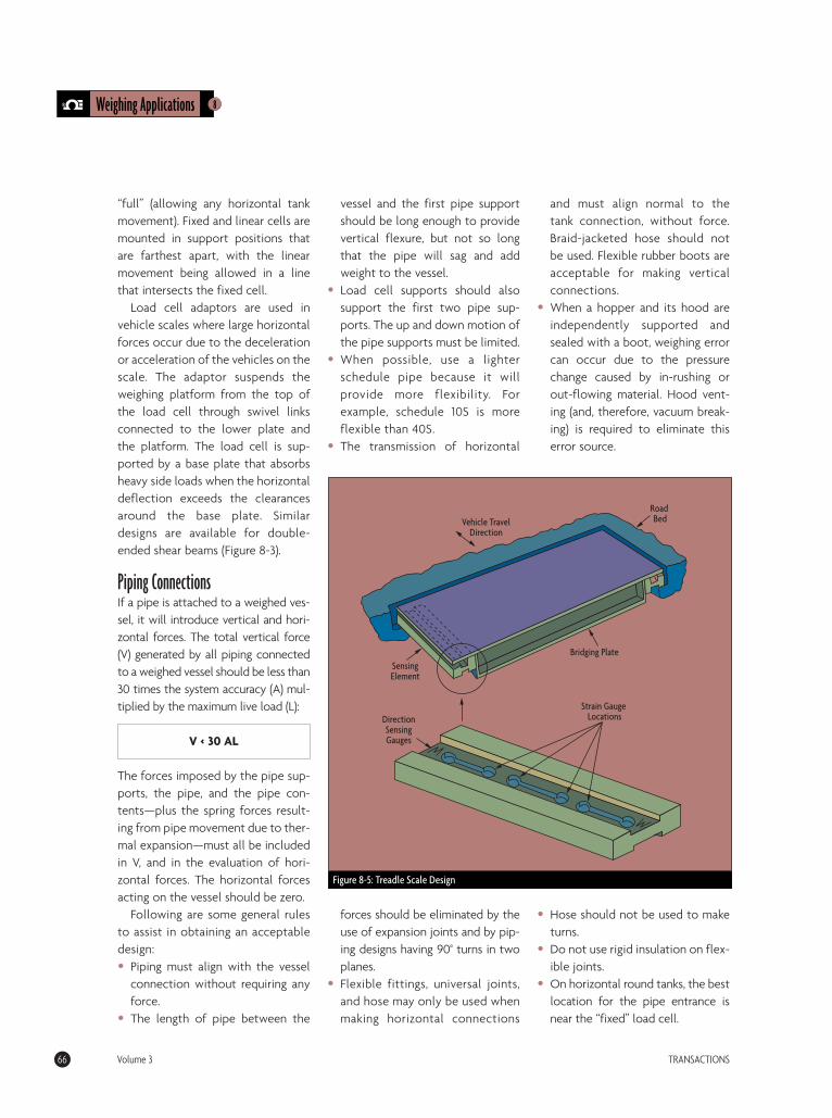
“full” (allowing any horizontal tankmovement). Fixed and linear cells aremounted in support positions thatare farthest apart, with the linearmovement being allowed in a linethat intersects the fixed cell.
Load cell adaptors are used invehicle scales where large horizontalforces occur due to the decelerationor acceleration of the vehicles on thescale. The adaptor suspends theweighing platform from the top ofthe load cell through swivel linksconnected to the lower plate andthe platform. The load cell is sup-ported by a base plate that absorbsheavy side loads when the horizontaldeflection exceeds the clearancesaround the base plate. Similardesigns are available for double-ended shear beams (Figure 8-3).
Piping Connections If a pipe is attached to a weighed ves-sel, it will introduce vertical and hori-zontal forces. The total vertical force(V) generated by all piping connectedto a weighed vessel should be less than30 times the system accuracy (A) mul-tiplied by the maximum live load (L):
V < 30 AL
The forces imposed by the pipe sup-ports, the pipe, and the pipe con-tents—plus the spring forces result-ing from pipe movement due to ther-mal expansion—must all be includedin V, and in the evaluation of hori-zontal forces. The horizontal forcesacting on the vessel should be zero.
Following are some general rulesto assist in obtaining an acceptabledesign: • Piping must align with the vessel
connection without requiring anyforce.
• The length of pipe between the
vessel and the first pipe supportshould be long enough to providevertical flexure, but not so longthat the pipe will sag and addweight to the vessel.
• Load cell supports should alsosupport the first two pipe sup-ports. The up and down motion ofthe pipe supports must be limited.
• When possible, use a lighterschedule pipe because it willprovide more flexibility. Forexample, schedule 10S is moreflexible than 40S.
• The transmission of horizontal
forces should be eliminated by theuse of expansion joints and by pip-ing designs having 90° turns in twoplanes.
• Flexible fittings, universal joints,and hose may only be used whenmaking horizontal connections
and must align normal to thetank connection, without force.Braid-jacketed hose should notbe used. Flexible rubber boots areacceptable for making verticalconnections.
• When a hopper and its hood areindependently supported andsealed with a boot, weighing errorcan occur due to the pressurechange caused by in-rushing orout-flowing material. Hood vent-ing (and, therefore, vacuum break-ing) is required to eliminate thiserror source.
• Hose should not be used to maketurns.
• Do not use rigid insulation on flex-ible joints.
• On horizontal round tanks, the bestlocation for the pipe entrance isnear the “fixed” load cell.
8Weighing Applications
66 Volume 3 TRANSACTIONS
Figure 8-5: Treadle Scale Design
Bridging Plate
Road Bed
Strain Gauge Locations
Vehicle Travel Direction
Sensing Element
Direction Sensing Gauges
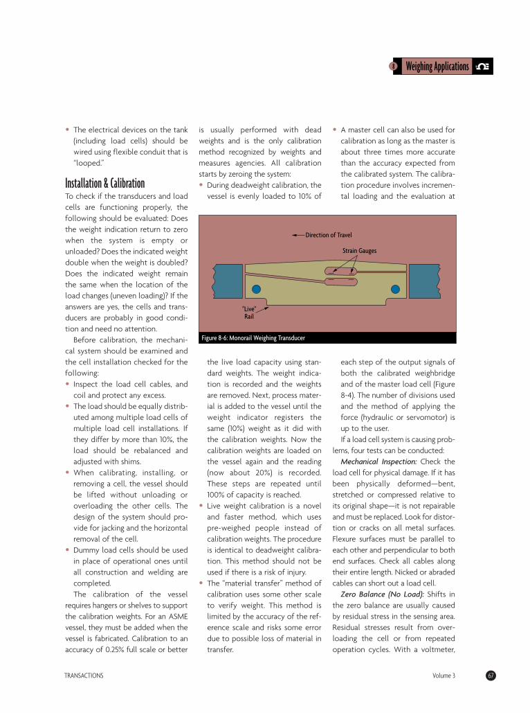
• The electrical devices on the tank(including load cells) should bewired using flexible conduit that is“looped.”
Installation & CalibrationTo check if the transducers and loadcells are functioning properly, thefollowing should be evaluated: Doesthe weight indication return to zerowhen the system is empty orunloaded? Does the indicated weightdouble when the weight is doubled?Does the indicated weight remainthe same when the location of theload changes (uneven loading)? If theanswers are yes, the cells and trans-ducers are probably in good condi-tion and need no attention.
Before calibration, the mechani-cal system should be examined andthe cell installation checked for thefollowing:• Inspect the load cell cables, and
coil and protect any excess.• The load should be equally distrib-
uted among multiple load cells ofmultiple load cell installations. Ifthey differ by more than 10%, theload should be rebalanced andadjusted with shims.
• When calibrating, installing, orremoving a cell, the vessel shouldbe lifted without unloading oroverloading the other cells. Thedesign of the system should pro-vide for jacking and the horizontalremoval of the cell.
• Dummy load cells should be usedin place of operational ones untilall construction and welding arecompleted. The calibration of the vessel
requires hangers or shelves to supportthe calibration weights. For an ASMEvessel, they must be added when thevessel is fabricated. Calibration to anaccuracy of 0.25% full scale or better
is usually performed with deadweights and is the only calibrationmethod recognized by weights andmeasures agencies. All calibrationstarts by zeroing the system:• During deadweight calibration, the
vessel is evenly loaded to 10% of
the live load capacity using stan-dard weights. The weight indica-tion is recorded and the weightsare removed. Next, process mater-ial is added to the vessel until theweight indicator registers thesame (10%) weight as it did withthe calibration weights. Now thecalibration weights are loaded onthe vessel again and the reading(now about 20%) is recorded.These steps are repeated until100% of capacity is reached.
• Live weight calibration is a noveland faster method, which usespre-weighed people instead ofcalibration weights. The procedureis identical to deadweight calibra-tion. This method should not beused if there is a risk of injury.
• The “material transfer” method ofcalibration uses some other scaleto verify weight. This method islimited by the accuracy of the ref-erence scale and risks some errordue to possible loss of material intransfer.
• A master cell can also be used forcalibration as long as the master isabout three times more accuratethan the accuracy expected fromthe calibrated system. The calibra-tion procedure involves incremen-tal loading and the evaluation at
each step of the output signals ofboth the calibrated weighbridgeand of the master load cell (Figure8-4). The number of divisions usedand the method of applying theforce (hydraulic or servomotor) isup to the user. If a load cell system is causing prob-
lems, four tests can be conducted: Mechanical Inspection: Check the
load cell for physical damage. If it hasbeen physically deformed—bent,stretched or compressed relative toits original shape—it is not repairableand must be replaced. Look for distor-tion or cracks on all metal surfaces.Flexure surfaces must be parallel toeach other and perpendicular to bothend surfaces. Check all cables alongtheir entire length. Nicked or abradedcables can short out a load cell.
Zero Balance (No Load): Shifts inthe zero balance are usually causedby residual stress in the sensing area.Residual stresses result from over-loading the cell or from repeatedoperation cycles. With a voltmeter,
8 Weighing Applications
TRANSACTIONS Volume 3 67
Figure 8-6: Monorail Weighing Transducer
Strain Gauges
Direction of Travel
"Live" Rail
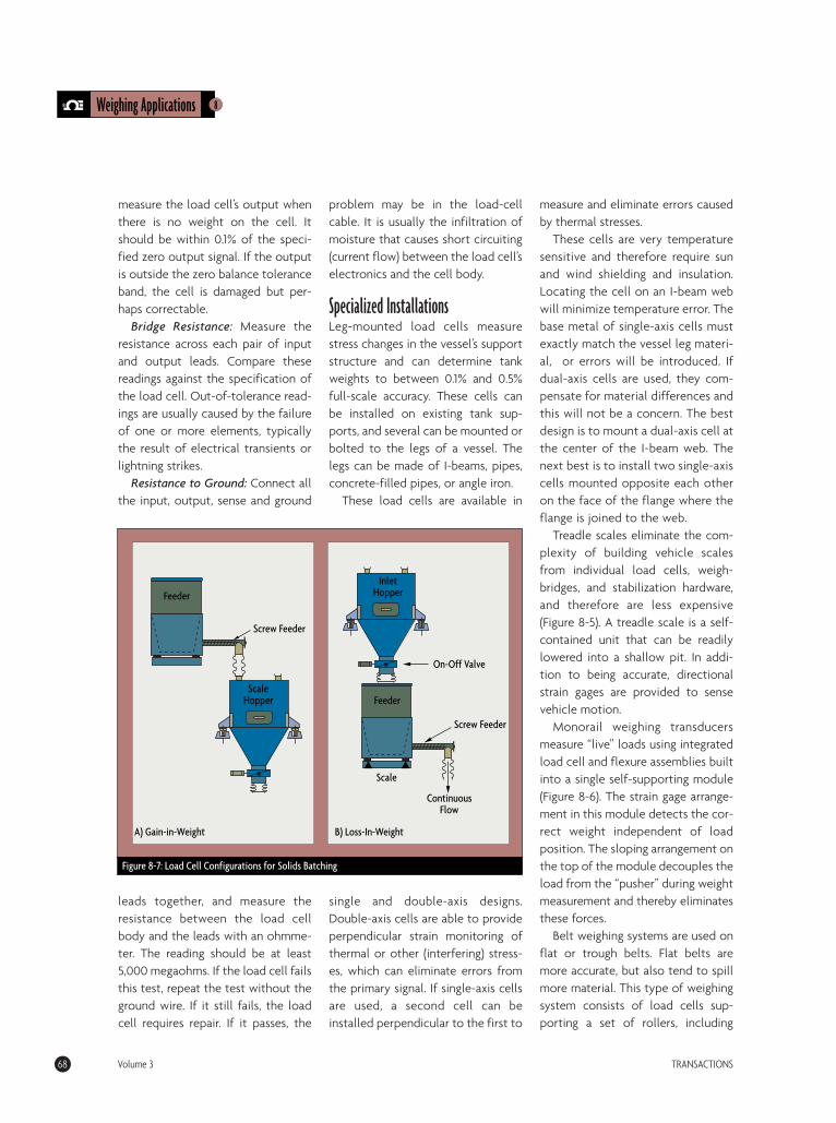
measure the load cell’s output whenthere is no weight on the cell. Itshould be within 0.1% of the speci-fied zero output signal. If the outputis outside the zero balance toleranceband, the cell is damaged but per-haps correctable.
Bridge Resistance: Measure theresistance across each pair of inputand output leads. Compare thesereadings against the specification ofthe load cell. Out-of-tolerance read-ings are usually caused by the failureof one or more elements, typicallythe result of electrical transients orlightning strikes.
Resistance to Ground: Connect allthe input, output, sense and ground
leads together, and measure theresistance between the load cellbody and the leads with an ohmme-ter. The reading should be at least5,000 megaohms. If the load cell failsthis test, repeat the test without theground wire. If it still fails, the loadcell requires repair. If it passes, the
problem may be in the load-cellcable. It is usually the infiltration ofmoisture that causes short circuiting(current flow) between the load cell’selectronics and the cell body.
Specialized Installations Leg-mounted load cells measurestress changes in the vessel’s supportstructure and can determine tankweights to between 0.1% and 0.5%full-scale accuracy. These cells canbe installed on existing tank sup-ports, and several can be mounted orbolted to the legs of a vessel. Thelegs can be made of I-beams, pipes,concrete-filled pipes, or angle iron.
These load cells are available in
single and double-axis designs.Double-axis cells are able to provideperpendicular strain monitoring ofthermal or other (interfering) stress-es, which can eliminate errors fromthe primary signal. If single-axis cellsare used, a second cell can beinstalled perpendicular to the first to
measure and eliminate errors causedby thermal stresses.
These cells are very temperaturesensitive and therefore require sunand wind shielding and insulation.Locating the cell on an I-beam webwill minimize temperature error. Thebase metal of single-axis cells mustexactly match the vessel leg materi-al, or errors will be introduced. Ifdual-axis cells are used, they com-pensate for material differences andthis will not be a concern. The bestdesign is to mount a dual-axis cell atthe center of the I-beam web. Thenext best is to install two single-axiscells mounted opposite each otheron the face of the flange where theflange is joined to the web.
Treadle scales eliminate the com-plexity of building vehicle scalesfrom individual load cells, weigh-bridges, and stabilization hardware,and therefore are less expensive(Figure 8-5). A treadle scale is a self-contained unit that can be readilylowered into a shallow pit. In addi-tion to being accurate, directionalstrain gages are provided to sensevehicle motion.
Monorail weighing transducersmeasure “live” loads using integratedload cell and flexure assemblies builtinto a single self-supporting module(Figure 8-6). The strain gage arrange-ment in this module detects the cor-rect weight independent of loadposition. The sloping arrangement onthe top of the module decouples theload from the “pusher” during weightmeasurement and thereby eliminatesthese forces.
Belt weighing systems are used onflat or trough belts. Flat belts aremore accurate, but also tend to spillmore material. This type of weighingsystem consists of load cells sup-porting a set of rollers, including
8Weighing Applications
68 Volume 3 TRANSACTIONS
Figure 8-7: Load Cell Configurations for Solids Batching
B) Loss-In-WeightA) Gain-in-Weight
Feeder
Screw Feeder
Scale Hopper
On-Off Valve
Screw Feeder
Continuous Flow
Scale
Feeder
Inlet Hopper
three idler rollers on either side thatstabilize and support the belt and itscontents as they move over thescale. Delivered weight is determinedby integrating the product of weightand belt speed signals.
The weighing system should belocated away from the material load-ing impact and spread area, and onthe opposite end from the drive pul-ley to avoid high belt tension. Beltsshould be single-ply, flexible, andshould track without lateral move-ment. The belt tension should bemaintained by weight-and-pulley tominimize jamming or resistance tomovement. Belt tension should beadjusted after monitoring the system’sresponse with more or less tension. Aloose belt causes side load errorbecause of belt slap or wrap, while atight belt can cause the load cell tomeasure belt tension instead of load.
Load cells are widely used inapplications requiring precisionweighing of solid and liquid materi-als. Depending on whether thereceiver or dispenser is beingweighed, these applications arereferred to as gain-in-weight or loss-in-weight configurations (Figure 8-7).
Loss-in-weight scales measure therate at which the total weight in thedispensing tank changes. They areused to control small mass flow ratesinto a process. These scales consistof a small load cell system, a differ-entiating measurement and controlsystem and a variable speed dis-penser. Normally, the speed of thedispenser is adjusted to maintain themass flow rate into the process; dur-ing the refill cycle, it is held constantat its last setting.
The scale hopper is weighed by loadcells connected via a summing box toa weight transmitter. The control sys-tem runs the screw feeder at a high
rate of speed (bulk rate) until the totaltarget weight is approached. At thatpoint the control system slows thescrew feeder down to a “dribble rate”.The screw feeder continues chargingat the dribble rate for a short period oftime, stopping just before the targetweight is attained.
The difference between the tar-get weight and the weight at whichthe screw feeder is stopped is calledthe “pre-act” weight. This pre-actdifference setting allows the con-trol system to consider the in-flightmaterial that is still falling from thescrew feeder into the scale hopper.The pre-act weight can be adjustedeither manually or automatically,and its correct setting is critical forhigh accuracy applications.
In the case of loss-in-weight batch-ing, a feeder is provided with an on-off valve at its inlet and with a variablespeed screw feeder at its outlet. The
entire feeder, including the inlet hop-per and the screw feeder, is mountedon load cells. When the feeder inletvalve is closed, the slope at which thetotal weight is dropping indicates thecontinuous discharge from the feeder.This slope is controlled by “loss-in-weight” controls, which calculate therate at which the total weight ischanging. The feed rate is set inpounds per hour, and the control sys-tem regulates the speed of the screwfeeder to maintain this desired dis-charge feed rate.
The control system speeds upthe screw feeder when the feedrate is below setpoint, and slows itdown when it is above setpoint.When the feeder is nearly empty,the control system switches thefeeder into its refill mode. In thismode, the inlet valve is opened andit is kept open until the desired fullweight is reached. T
8 Weighing Applications
TRANSACTIONS Volume 3 69
References & Further Reading• Omegadyne®Pressure, Force, Load, Torque Databook, OMEGADYNE, Inc.,
1996.• The Pressure, Strain, and Force Handbook™, Omega Press LLC, 1996.• “How to troubleshoot your electronic scale,” Brent Yeager, Powder and
Bulk Engineering, September, 1995 • “Ten rules for installing a belt scale”, Steve Becker, Powder and Bulk
Engineering, September, 1996.• “Flat-belt weigh feeder accuracy: How to achieve it, maintain it, and ver-
ify it”, Pete Cadou and Chuck Homer, Powder and Bulk Engineering,September, 1997.
• Electronic Weigh Systems Handbook, BLH Electronics, 1986.• Instrument Engineers’ Handbook, Bela Liptak, CRC Press LLC, 1995. • Marks’ Standard Handbook for Mechanical Engineers, 10th Edition,
Eugene A. Avallone and Theodore Baumeister, McGraw-Hill, 1996.• McGraw-Hill Concise Encyclopedia of Science and Technology, McGraw-
Hill, 1998.• Process/Industrial Instruments and Controls Handbook, 4th Edition,
Douglas M. Considine, McGraw-Hill, 1993.• Van Nostrand’s Scientific Encyclopedia, Douglas M. Considine and Glenn
D. Considine, Van Nostrand, 1997• Weighing and Force Measurement in the 90’s, IMEKO TC, 1991.

Information Resources
70 Volume 3 TRANSACTIONS
American Institute of Chemical Engineers (AIChE)345 East 47 Street, New York, NY 10017-2395 212/705-7338 www.aiche.org
American National Standards Institute (ANSI)11 West 42 Street, New York, NY 10036 212/642-4900 www.ansi.org
American Society of Mechanical Engineers (ASME)345 East 47 Street, New York, NY 10017 212/705-7722 www.asme.org
American Society for Testing and Materials (ASTM)100 Barr Harbor Drive, West Conshohocken, PA 19428-2959 610/832-9585 www.astm.org
American Vacuum Society (AVS)120 Wall Street, 32nd Floor, New York, NY 10005 212/248-0200 www.vacuum.org
Electric Power Research Institute (EPRI)3412 Hillview Avenue, Palo Alto, CA 94303 415/855-2000 www.epri.com
Electronic Industries Association (EIA)2500 Wilson Boulevard, Arlington, VA 22201-3834 703/907-7500 www.eia.org
Factory Mutual1151 Boston-Providence Turnpike, Norwood, MA 02062 781/762-4300 www.factorymutual.com
International Electrotechnical Commission (IEC)3, rue de Varembé, P.O. Box 131 +41 22 919 02 11 www.iec.chCH - 1211 Geneva 20, Switzerland
International Organization for Standardization (ISO)1, rue de Varembé, Case postale 56, +41 22 749 01 11 www.iso.chCH-1211 Geneva 20, Switzerland
Institute of Electrical & Electronics Engineers (IEEE)445 Hoes Lane, Piscataway, NJ 08855-1331 732/981-0060 www.ieee.org
ISA—The International Society for Measurement and Control67 Alexander Drive, Research Triangle Park, NC 27709 919/549-8411 www.isa.org
National Electrical Manufacturers Association (NEMA)1300 North 17th Street, Suite 1847, Rosslyn, VA 22209 703/841-3200 www.nema.org
National Fire Protection Association (NFPA)1 Batterymarch Park, Quincy, MA 02269-9101 617/770-3000 www.nfpa.org
National Institute of Standards and TechnologyGaithersburg, MD 20899-0001 301/975-3058 www.nist.gov
Society of Automotive Engineers (SAE)400 Commonwealth Drive, Warrendale, PA 15096-0001 724/776-4841 www.sae.org
Underwriters Laboratories333 Pfingsten Road, Northbrook, IL 60062 847/272-8800 www.ul.com
Information ResourcesORGANIZATIONSNAME/ADDRESS PHONE WEB ADDRESS
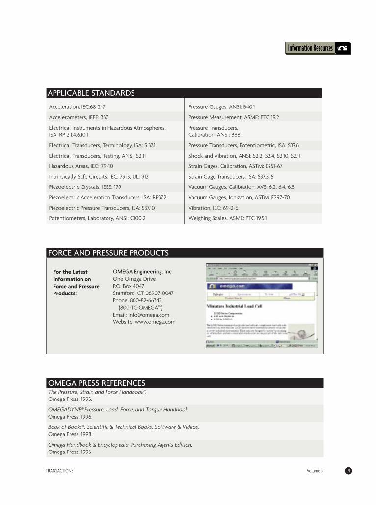
Information Resources
TRANSACTIONS Volume 3 71
Information Resources
OMEGA PRESS REFERENCES
For the LatestInformation onForce and PressureProducts:
OMEGA Engineering, Inc.One Omega DriveP.O. Box 4047 Stamford, CT 06907-0047Phone: 800-82-66342
(800-TC-OMEGASM)Email: [email protected]: www.omega.com
APPLICABLE STANDARDS
Acceleration, IEC:68-2-7
Accelerometers, IEEE: 337
Electrical Instruments in Hazardous Atmospheres, ISA: RP12.1,4,6,10,11
Electrical Transducers, Terminology, ISA: S.37.1
Electrical Transducers, Testing, ANSI: S2.11
Hazardous Areas, IEC: 79-10
Intrinsically Safe Circuits, IEC: 79-3, UL: 913
Piezoelectric Crystals, IEEE: 179
Piezoelectric Acceleration Transducers, ISA: RP37.2
Piezoelectric Pressure Transducers, ISA: S37.10
Potentiometers, Laboratory, ANSI: C100.2
Pressure Gauges, ANSI: B40.1
Pressure Measurement, ASME: PTC 19.2
Pressure Transducers, Calibration, ANSI: B88.1
Pressure Transducers, Potentiometric, ISA: S37.6
Shock and Vibration, ANSI: S2.2, S2.4, S2.10, S2.11
Strain Gages, Calibration, ASTM: E251-67
Strain Gage Transducers, ISA: S37.3, 5
Vacuum Gauges, Calibration, AVS: 6.2, 6.4, 6.5
Vacuum Gauges, Ionization, ASTM: E297-70
Vibration, IEC: 69-2-6
Weighing Scales, ASME: PTC 19.5.1
FORCE AND PRESSURE PRODUCTS
The Pressure, Strain and Force Handbook™, Omega Press, 1995.
OMEGADYNE® Pressure, Load, Force, and Torque Handbook, Omega Press, 1996.
Book of Books®: Scientific & Technical Books, Software & Videos, Omega Press, 1998.
Omega Handbook & Encyclopedia, Purchasing Agents Edition, Omega Press, 1995

Information Resources
72 Volume 3 TRANSACTIONS
Electrical Measuring Instruments C.V. Drysdale and A.C. Jolley, Ernest Bern, 1924
Electrical Measurements and Measuring Instruments E.W. Goldin, Pitman and Sons, 1948
Electrical Measurements F.K. Harris, Wiley, 1952
Electronic Test Instruments Robert Witte, Prentice Hall, 1993
Electronic Weighing K. Ellis Norden, Butterworth-Heinemann, 1993
Electronic Weigh System Handbook BLH Electronics, 1979
Elements of Electronic Instrumentation and Measurements, 3rd edition Joseph J. Carr editor, Prentice Hall, 1996
The Examination of Weighing Equipment NBS Handbook No. 94, 1965
Handbook of Intelligent Sensors for Industrial Automation Nello Zuech, Addison-Wesley Publishing, 1992
Handbook of Transducers Harry N. Norton, Prentice Hall, 1989
Industrial Control Handbook E.A. Parr editor, Butterworth-Heinemann Ltd., 1995
Industrial Pressure Measurement D.R. Gillum, ISA, 1982
Industrial Weighing D.M. Considine, Reinhold, 1948
Instrumentation and Control C.L. Nachtigal, Wiley, 1990
Instrumentation and Process Control Nicholas P. Chopey, McGraw-Hill, 1996
Instrumentation for Engineering Measurements J. Dally, Wiley, 1993
Instrumentation for Process Measurement and Control, 3rd edition Norman A. Andreson, 1980
Instrumentation in Industry H.E. Soisson, Wiley, 1975
Instrumentation Reference Book, 2nd edition B.E. Noltingk editor, Butterworth-Heinemann, 1995
Instrument Engineer’s Handbook, Process Measurement Volume, 3rd edition Bela Liptak editor, CRC Press, 1995
The McGraw-Hill Encyclopedia of Science and Technology, 8th edition McGraw-Hill, 1997
OTHER REFERENCE BOOKS

Information Resources
TRANSACTIONS Volume 3 73
OTHER REFERENCE BOOKSMeasurement and Competitiveness in Electronics NIST Electronics and Electrical Engineering Laboratory, 1993
Measurement and Control Basics, 2nd editionT.A. Hughes, ISA, 1995
Mechanical Problems in Measuring Force and Mass H. Wieringa, Martinus Nijhoff Publishers, 1986
National Electrical Safety CodeIEEE, 1993
Notable Twentieth-Century Scientists Emily J. McMurray, Gale Research Inc., 1995
Pioneers of Modern Science, The World of Science Bill MacKeith, Andromeda Oxford Limited, 1991
Pressure Gauge Handbook Philip W. Harland, Marcel Dekker, 1991
Principles of Industrial Measurement and Control Applications E. Smith, ISA, 1984
Process/Industrial Instruments and Controls, 4th editionDouglas M. Considine, McGraw-Hill, 1993
Process Measurement and Analysis, Instrument Engineers’ Handbook, 3rd edition Bela Liptak editor, CRC Press, 1995
The Scientific 100, A Ranking of the Most Influential Scientists, Past and PresentJohn Simmons, Carol Publishing Group, 1996
Sensor and Analyzer Handbook H.N. Norton, Prentice-Hall, 1982
Sensors and Control Systems in Manufacturing S. Soloman, McGraw-Hill, 1994
The Strain Gauge Primer C.C. Perry and H.R. Lissner, McGraw-Hill, 1962
Van Nostrand’s Scientific EncyclopediaDouglas M. Considine, Van Nostrand, 1995
Vibration Analysis for Electronic Equipment, 2nd edition Dave S. Steinberg, Wiley, 1988
Weighing and Batching of Bulk SolidsH. Colijn editor, Trans Tech Publications, 1975
Weighing and Force Measurement in the 90’sT. Kemeny editor, IMEKO TC Series, 1991
Teflon® is a registered trademark of DuPont.
Glossary
74 Volume 3 TRANSACTIONS
Absolute pressure: Pressure referenced to full vacuum. InEnglish (pounds per square inch) units, designated as PIA.Accuracy: Degree of conformity of a measured value toan accepted standard value or closeness of a reading orindication of a sensor to the actual value of the quantitybeing measured.Accuracy rating: A number that defines a limit that themeasurement errors will not exceed under some refer-ence operating conditions. It includes the combinedeffects of conformity, hysteresis, dead band and repeata-bility errors. Accuracy, units: The maximum positive or negative devi-ation (inaccuracy) observed in testing a device. It can beexpressed in terms of the measured variable (plus-minus1°C), or as a percentage of the actual reading (%AR), ofthe full scale (%FS), of upper range value (%URL), of thespan or of scale length. Admittance: Admittance of an AC circuit is analogous tothe conductivity of a DC circuit; it is the reciprocal of theimpedance of an AC circuit.Air consumption: The maximum rate at which air is con-sumed by an instrument while operating within its oper-ating range, usually expressed in units of standard cubicfeet per minute.Alphanumeric: A character set containing both lettersand numbers.Alternating current (AC): A flow of electric charge (elec-tric current) that undergoes periodic reverses in direc-tion. In North America, the household current alternatesat a frequency of 60 times per second.Ambient pressure: The atmospheric pressure of themedium surrounding a particular sensor. When no spe-cific information is available, it is assumed to be 14.7 PSIA.Ambient temperature: The average or mean tempera-ture of the atmospheric air which is surrounding a sen-sor or instrument. If the sensor is a heat generator, thisterm refers to the temperature of the surroundingswhen the sensor is in operation. The ambient tempera-ture is usually stated under the assumption that thesensor is not exposed to the sun or other radiant ener-gy sources. Ambient temperature compensation: An automaticcorrection which prevents the reading of a sensor or
instrument from being affected by variations in ambi-ent temperature. The compensator specifications statethe temperature range within which the compensationis effective. American National Standards Institute (ANSI): A profes-sional organization in the United States responsible foraccepting and designating the standards developed byother organizations as national standards.Ampere (A or amp): The unit of electric current flow,defined as the rate at which one coulomb of electriccharge (6.25x10¹⁸ electrons) is transferred in a second.Amplifier: A device that generates an output which isstronger than and bears some predetermined relation-ship (often linear) to its input. It generates the amplifiedoutput signal while drawing power from a source otherthan the signal itself. Analog signal: A signal that continuously represents avariable or condition.Analog-to-digital (A/D) conversion: A generic termreferring to the conversion of an analog signal into a dig-ital form.Analog-to-digital converter (ADC): An electronic devicethat converts analog signals to an equivalent digital form.Attenuation: The reciprocal of gain; a dimensionlessratio defining the decrease in signal magnitude as it pass-es between two points or two frequencies. Large valuesof attenuation are expressed in decibels (dB).
Backlash: The relative movement of interlocked mechan-ical parts which occurs when motion is reversed.Baud rate: Serial communications data transmission rateexpressed in bits per second (bps).Bipolar: A signal range that includes both positive andnegative values (i.e., -10 V to +10 V).Bode diagram: A plot of log amplitude ratio and phaseangle values used in describing transfer functions. Breakdown voltage: Threshold voltage at which circuitcomponents begin to be damaged.Byte (B): Eight related bits of data or an eight-bit binarynumber. Also denotes the amount of memory requiredto store one byte of data.
Calibrate: To ascertain that the output of a device prop-erly corresponds to the information it is measuring,
A
B
Glossary
C
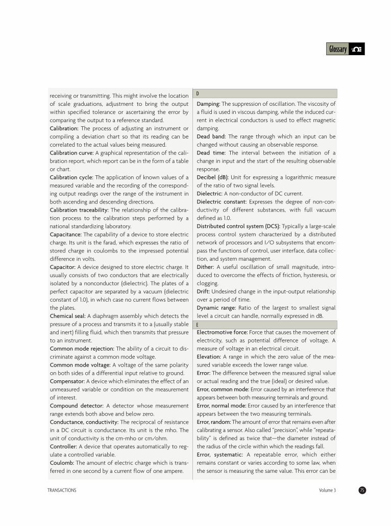
Glossary
TRANSACTIONS Volume 3 75
receiving or transmitting. This might involve the locationof scale graduations, adjustment to bring the outputwithin specified tolerance or ascertaining the error bycomparing the output to a reference standard.Calibration: The process of adjusting an instrument orcompiling a deviation chart so that its reading can becorrelated to the actual values being measured. Calibration curve: A graphical representation of the cali-bration report, which report can be in the form of a tableor chart.Calibration cycle: The application of known values of ameasured variable and the recording of the correspond-ing output readings over the range of the instrument inboth ascending and descending directions.Calibration traceability: The relationship of the calibra-tion process to the calibration steps performed by anational standardizing laboratory.Capacitance: The capability of a device to store electriccharge. Its unit is the farad, which expresses the ratio ofstored charge in coulombs to the impressed potentialdifference in volts. Capacitor: A device designed to store electric charge. Itusually consists of two conductors that are electricallyisolated by a nonconductor (dielectric). The plates of aperfect capacitor are separated by a vacuum (dielectricconstant of 1.0), in which case no current flows betweenthe plates.Chemical seal: A diaphragm assembly which detects thepressure of a process and transmits it to a (usually stableand inert) filling fluid, which then transmits that pressureto an instrument. Common mode rejection: The ability of a circuit to dis-criminate against a common mode voltage.Common mode voltage: A voltage of the same polarityon both sides of a differential input relative to ground.Compensator: A device which eliminates the effect of anunmeasured variable or condition on the measurementof interest. Compound detector: A detector whose measurementrange extends both above and below zero. Conductance, conductivity: The reciprocal of resistancein a DC circuit is conductance. Its unit is the mho. Theunit of conductivity is the cm-mho or cm/ohm.Controller: A device that operates automatically to reg-ulate a controlled variable.Coulomb: The amount of electric charge which is trans-ferred in one second by a current flow of one ampere.
Damping: The suppression of oscillation. The viscosity ofa fluid is used in viscous damping, while the induced cur-rent in electrical conductors is used to effect magneticdamping. Dead band: The range through which an input can bechanged without causing an observable response.Dead time: The interval between the initiation of achange in input and the start of the resulting observableresponse. Decibel (dB): Unit for expressing a logarithmic measureof the ratio of two signal levels. Dielectric: A non-conductor of DC current.Dielectric constant: Expresses the degree of non-con-ductivity of different substances, with full vacuumdefined as 1.0.Distributed control system (DCS): Typically a large-scaleprocess control system characterized by a distributednetwork of processors and I/O subsystems that encom-pass the functions of control, user interface, data collec-tion, and system management. Dither: A useful oscillation of small magnitude, intro-duced to overcome the effects of friction, hysteresis, orclogging.Drift: Undesired change in the input-output relationshipover a period of time.Dynamic range: Ratio of the largest to smallest signallevel a circuit can handle, normally expressed in dB.
Electromotive force: Force that causes the movement ofelectricity, such as potential difference of voltage. Ameasure of voltage in an electrical circuit.Elevation: A range in which the zero value of the mea-sured variable exceeds the lower range value. Error: The difference between the measured signal valueor actual reading and the true (ideal) or desired value. Error, common mode: Error caused by an interference thatappears between both measuring terminals and ground.Error, normal mode: Error caused by an interference thatappears between the two measuring terminals.Error, random: The amount of error that remains even aftercalibrating a sensor. Also called “precision”, while “repeata-bility” is defined as twice that—the diameter instead ofthe radius of the circle within which the readings fall.Error, systematic: A repeatable error, which eitherremains constant or varies according to some law, whenthe sensor is measuring the same value. This error can be
D
E
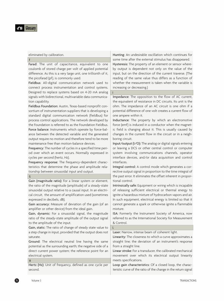
Glossary
76 Volume 3 TRANSACTIONS
eliminated by calibration.
Farad: The unit of capacitance, equivalent to onecoulomb of stored charge per volt of applied potentialdifference. As this is a very large unit, one trillionth of it,the picofarad (pf), is commonly used.Fieldbus: All-digital communication network used toconnect process instrumentation and control systems.Designed to replace systems based on 4-20 mA analogsignals with bidirectional, multivariable data communica-tion capability.Fieldbus Foundation: Austin, Texas-based nonprofit con-sortium of instrumentation suppliers that is developing astandard digital communication network (fieldbus) forprocess control applications. The network developed bythe Foundation is referred to as the Foundation Fieldbus. Force balance: Instruments which operate by force-bal-ance between the detected variable and the generatedoutput require no motion and therefore tend to be moremaintenance free than motion-balance devices. Frequency: The number of cycles in a specified time peri-od over which an event occurs. Normally expressed incycles per second (hertz, Hz).Frequency response: The frequency-dependent charac-teristics that determine the phase and amplitude rela-tionship between sinusoidal input and output.
Gain (magnitude ratio): For a linear system or element,the ratio of the magnitude (amplitude) of a steady-statesinusoidal output relative to a causal input. In an electri-cal circuit, the amount of amplification used (sometimesexpressed in decibels, dB).Gain accuracy: Measure of deviation of the gain (of anamplifier or other device) from the ideal gain. Gain, dynamic: For a sinusoidal signal, the magnituderatio of the steady-state amplitude of the output signalto the amplitude of the input.Gain, static: The ratio of change of steady state value toa step change in input, provided that the output does notsaturate. Ground: The electrical neutral line having the samepotential as the surrounding earth; the negative side of adirect current power system; the reference point for anelectrical system.
Hertz (Hz): Unit of frequency, defined as one cycle persecond.
Hunting: An undesirable oscillation which continues forsome time after the external stimulus has disappeared.Hysteresis: The property of an element or sensor where-by output is dependent not only on the value of theinput, but on the direction of the current traverse. (Thereading of the same value thus differs as a function ofwhether the measurement is taken when the variable isincreasing or decreasing.)
Impedance: The opposition to the flow of AC current,the equivalent of resistance in DC circuits. Its unit is theohm. The impedance of an AC circuit is one ohm if apotential difference of one volt creates a current flow ofone ampere within it.Inductance: The property by which an electromotiveforce (emf) is induced in a conductor when the magnet-ic field is changing about it. This is usually caused bychanges in the current flow in the circuit or in a neigh-boring circuit.Input/output (I/O): The analog or digital signals enteringor leaving a DCS or other central control or computersystem involving communications channels, operatorinterface devices, and/or data acquisition and controlinterfaces. Integral control: A control mode which generates a cor-rective output signal in proportion to the time integral ofthe past error. It eliminates the offset inherent in propor-tional control. Intrinsically safe: Equipment or wiring which is incapableof releasing sufficient electrical or thermal energy toignite a hazardous mixture of hydrocarbon vapors and air.In such equipment, electrical energy is limited so that itcannot generate a spark or otherwise ignite a flammablemixture. ISA: Formerly the Instrument Society of America, nowreferred to as the International Society for Measurement& Control.
Laser: Narrow, intense beam of coherent light.Linearity: The closeness to which a curve approximates astraight line; the deviation of an instrument’s responsefrom a straight line. Linear stroke: For a transducer, the calibrated mechanicalmovement over which its electrical output linearitymeets specifications.Loop gain characteristics: Of a closed loop, the charac-teristic curve of the ratio of the change in the return signal
I
F
G
L
H
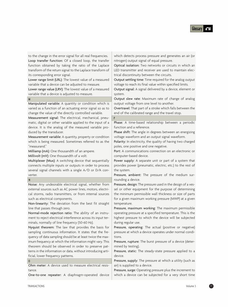
Glossary
TRANSACTIONS Volume 3 77
to the change in the error signal for all real frequencies.Loop transfer function: Of a closed loop, the transferfunction obtained by taking the ratio of the Laplacetransform of the return signal to the Laplace transform ofits corresponding error signal.Lower range limit (LRL): The lowest value of a measuredvariable that a device can be adjusted to measure.Lower range value (LRV): The lowest value of a measuredvariable that a device is adjusted to measure.
Manipulated variable: A quantity or condition which isvaried as a function of an actuating error signal so as tochange the value of the directly controlled variable.Measurement signal: The electrical, mechanical, pneu-matic, digital or other variable applied to the input of adevice. It is the analog of the measured variable pro-duced by the transducer.Measurement variable: A quantity, property or conditionwhich is being measured. Sometimes referred to as the“measurand.”Milliamp (mA): One thousandth of an ampere.Millivolt (mV): One thousandth of a volt.Multiplexer (Mux): A switching device that sequentiallyconnects multiple inputs or outputs in order to processseveral signal channels with a single A/D or D/A con-verter.
Noise: Any undesirable electrical signal, whether fromexternal sources such as AC power lines, motors, electri-cal storms, radio transmitters, or from internal sourcessuch as electrical components.Non-linearity: The deviation from the best fit straightline that passes through zero.Normal-mode rejection ratio: The ability of an instru-ment to reject electrical interference across its input ter-minals, normally of line frequency (50-60 Hz).Nyquist theorem: The law that provides the basis forsampling continuous information. It states that the fre-quency of data sampling should be at least twice the max-imum frequency at which the information might vary. Thistheorem should be observed in order to preserve pat-terns in the information or data, without introducing arti-ficial, lower frequency patterns.
Ohm meter: A device used to measure electrical resis-tance.One-to-one repeater: A diaphragm-operated device
which detects process pressure and generates an air (ornitrogen) output signal of equal pressure.Optical isolation: Two networks or circuits in which anLED transmitter and receiver are used to maintain elec-trical discontinuity between the circuits.Output settling time: Time required for the analog outputvoltage to reach its final value within specified limits. Output signal: A signal delivered by a device, element orsystem.Output slew rate: Maximum rate of change of analogoutput voltage from one level to another. Overtravel: That part of a stroke which falls between theend of the calibrated range and the travel stop.
Phase: A time-based relationship between a periodicfunction and a reference. Phase shift: The angle in degrees between an energizingvoltage waveform and an output signal waveform.Polarity: In electricity, the quality of having two chargedpoles, one positive and one negative.Port: A communications connection on an electronic orcomputer-based device.Power supply: A separate unit or part of a system thatprovides power (pneumatic, electric, etc.) to the rest ofthe system.Pressure, ambient: The pressure of the medium sur-rounding a device.Pressure, design: The pressure used in the design of a ves-sel or other equipment for the purpose of determiningthe minimum permissible wall thickness or size of partsfor a given maximum working pressure (MWP) at a giventemperature.Pressure, maximum working: The maximum permissibleoperating pressure at a specified temperature. This is thehighest pressure to which the device will be subjectedduring regular use. Pressure, operating: The actual (positive or negative)pressure at which a device operates under normal condi-tions.Pressure, rupture: The burst pressure of a device (deter-mined by testing).Pressure, static: The steady-state pressure applied to adevice. Pressure, supply: The pressure at which a utility (such asair) is supplied to a device.Pressure, surge: Operating pressure plus the increment towhich a device can be subjected for a very short time
O
P
M
N
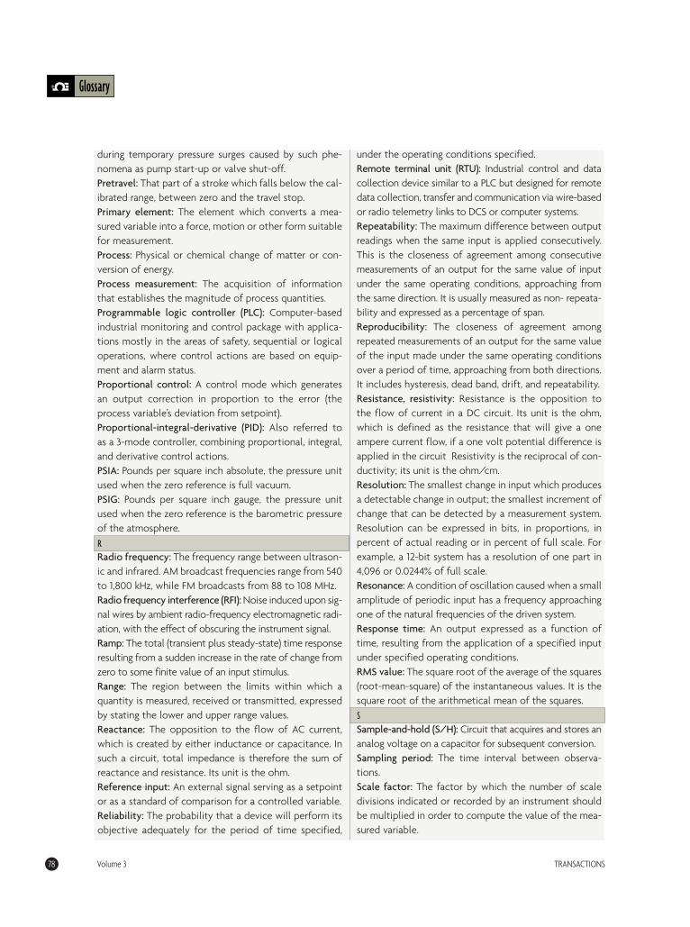
Glossary
78 Volume 3 TRANSACTIONS
during temporary pressure surges caused by such phe-nomena as pump start-up or valve shut-off.Pretravel: That part of a stroke which falls below the cal-ibrated range, between zero and the travel stop. Primary element: The element which converts a mea-sured variable into a force, motion or other form suitablefor measurement.Process: Physical or chemical change of matter or con-version of energy.Process measurement: The acquisition of informationthat establishes the magnitude of process quantities.Programmable logic controller (PLC): Computer-basedindustrial monitoring and control package with applica-tions mostly in the areas of safety, sequential or logicaloperations, where control actions are based on equip-ment and alarm status. Proportional control: A control mode which generatesan output correction in proportion to the error (theprocess variable’s deviation from setpoint).Proportional-integral-derivative (PID): Also referred toas a 3-mode controller, combining proportional, integral,and derivative control actions. PSIA: Pounds per square inch absolute, the pressure unitused when the zero reference is full vacuum.PSIG: Pounds per square inch gauge, the pressure unitused when the zero reference is the barometric pressureof the atmosphere.
Radio frequency: The frequency range between ultrason-ic and infrared. AM broadcast frequencies range from 540to 1,800 kHz, while FM broadcasts from 88 to 108 MHz. Radio frequency interference (RFI): Noise induced upon sig-nal wires by ambient radio-frequency electromagnetic radi-ation, with the effect of obscuring the instrument signal. Ramp: The total (transient plus steady-state) time responseresulting from a sudden increase in the rate of change fromzero to some finite value of an input stimulus.Range: The region between the limits within which aquantity is measured, received or transmitted, expressedby stating the lower and upper range values.Reactance: The opposition to the flow of AC current,which is created by either inductance or capacitance. Insuch a circuit, total impedance is therefore the sum ofreactance and resistance. Its unit is the ohm.Reference input: An external signal serving as a setpointor as a standard of comparison for a controlled variable. Reliability: The probability that a device will perform itsobjective adequately for the period of time specified,
under the operating conditions specified. Remote terminal unit (RTU): Industrial control and datacollection device similar to a PLC but designed for remotedata collection, transfer and communication via wire-basedor radio telemetry links to DCS or computer systems.Repeatability: The maximum difference between outputreadings when the same input is applied consecutively.This is the closeness of agreement among consecutivemeasurements of an output for the same value of inputunder the same operating conditions, approaching fromthe same direction. It is usually measured as non- repeata-bility and expressed as a percentage of span.Reproducibility: The closeness of agreement amongrepeated measurements of an output for the same valueof the input made under the same operating conditionsover a period of time, approaching from both directions.It includes hysteresis, dead band, drift, and repeatability.Resistance, resistivity: Resistance is the opposition tothe flow of current in a DC circuit. Its unit is the ohm,which is defined as the resistance that will give a oneampere current flow, if a one volt potential difference isapplied in the circuit Resistivity is the reciprocal of con-ductivity; its unit is the ohm/cm.Resolution: The smallest change in input which producesa detectable change in output; the smallest increment ofchange that can be detected by a measurement system.Resolution can be expressed in bits, in proportions, inpercent of actual reading or in percent of full scale. Forexample, a 12-bit system has a resolution of one part in4,096 or 0.0244% of full scale.Resonance: A condition of oscillation caused when a smallamplitude of periodic input has a frequency approachingone of the natural frequencies of the driven system.Response time: An output expressed as a function oftime, resulting from the application of a specified inputunder specified operating conditions.RMS value: The square root of the average of the squares(root-mean-square) of the instantaneous values. It is thesquare root of the arithmetical mean of the squares.
Sample-and-hold (S/H): Circuit that acquires and stores ananalog voltage on a capacitor for subsequent conversion. Sampling period: The time interval between observa-tions.Scale factor: The factor by which the number of scaledivisions indicated or recorded by an instrument shouldbe multiplied in order to compute the value of the mea-sured variable.
R
S
Glossary
TRANSACTIONS Volume 3 79
SCFM: Standard cubic foot per minute, where the term“standard” usually refers to 14.7 PSIA pressure and 68°Ftemperature.Sensing element: The element which is directly respon-sive to the value of the measured variable.Sensitivity: The minimum change in a physical variableto which an instrument can respond; the ratio of thechange in output magnitude to the change of the inputwhich causes it after steady-state has been reached.Sensor: An element or device which detects a variable,receiving information in the form of one quantity andconverting it to information in the form of that oranother quantity. Servomechanism: An automatic feedback device inwhich the controlled variable is mechanical position orany of its time derivatives.Setpoint: A variable, expressed in the same units as themeasurement to be taken, which sets either the desiredtarget for a controller or the condition at which alarmsor safety interlocks are to be energized.Settling time: The time required after a stimulus for theoutput to center and remain within a specified narrowband centered on its steady-state value.Shielded twisted pair (STP): Cable construction thatincludes an external grounded shield as well as twistingon a regular basis to minimize noise.Signal: A variable that carries information about anothervariable that it represents.Signal-to-noise ratio: Ratio of signal amplitude to noiseamplitude; the ratio of the overall rms signal level to therms noise level, expressed in dB. For sinusoidal signals,amplitude may be peak or rms.Single-ended (SE): An analog input that is measured withrespect to a common ground. Span: The algebraic difference between the upper andlower range values, expressed in the same units as therange.Span shift: Any change in slope of the input-outputcurve.Stability: The ability of an instrument or sensor to main-tain a consistent output when a constant input isapplied.Steady-state: A characteristic of a condition, such asvalue, rate, periodicity, or amplitude, exhibiting only neg-ligible change over an arbitrary long period of time.Stiffness: The ratio of change of force (or torque) to theresulting change in deflection of a spring-like element;the opposite of compliance.
Strain: The ratio of the change in length to the initialunstressed reference length of an element under stress.Strain gage: Sensor whose resistance varies with appliedforce. A measuring element for converting force, pressure,tension, weight, etc., into a change in electrical resistance. Subsidence: The progressive reduction or suppression ofoscillation in a device or system.Suppressed range: The range in which the zero value of ameasured variable is greater than the lower-range value(LRV). The terms “elevated zero,” “suppression” or “sup-pressed span” are also used to express the condition thatexists when the zero of the measured variable is greaterthan the LRV.Suppressed span: The span in which the zero of the mea-sured variable is greater than the LRV.Suppressed zero: The range in which the zero value of themeasured variable is less than the lower range value. Theterms “elevation,” “elevated range” and “elevated span” arefrequently used to express the condition in which the zeroof the measured variable is less than the lower range value. Suppression ratio: The ratio of the lower-range value tothe span. If range is 20-100 and therefore span is 80 andLRV is 20, the suppression ratio is 20/80 = 0.25 or 25%.Synchronous: An event or action that is synchronized toa reference clock. System noise: The measure of the amount of noise seenby an analog circuit or an ADC when the analog inputsare grounded.
Temperature coefficient: The amount of drift, in percentof full scale output, that might result from a 1°C changein ambient temperature. Thermal shock: An abrupt temperature change appliedto a device.Time constant: The value T in an exponential term A(-t/T).For the output of a first-order system forced by a step oran impulse, T is the time required to complete 63.2% ofthe total rise or decay. For higher order systems, there isa time constant for each of the first-order componentsof the process. Torque tube: A torsion spring used to measure force orpressure.Transducer: An element or device which receives infor-mation in the form of one quantity and converts it toinformation in the same or another quantity or form.Primary elements and transmitters are also referred to astransducers.Transfer function: Mathematical, graphical, or tabular
T
Glossary
80 Volume 3 TRANSACTIONS
statement of the influence which a system or elementhas on a signal or action compared at input and at out-put terminals.Transient: The behavior of a variable during transitionbetween two steady-states.Transmitter: A transducer which responds to a measuredvariable by means of a sensing element, and converts itto a standardized transmission signal which is a functiononly of the values of the measured variable.
Upper range limit (URL): The highest value of a measuredvariable that a device can be adjusted to measure. (Thisvalue corresponds to the top of the range.)Upper range value (URV): The highest value of a mea-sured variable that a device is adjusted to measure. (Thisvalue corresponds to the top of the span.)
Vapor pressure: The pressure exerted by a vapor which isin equilibrium with its own liquid.Variable: Any condition which is measured, controlled(directly or indirectly) or manipulated.Velocity limit: A limit on the rate of change, which a par-ticular variable may not exceed.Vibration: A periodic motion or oscillation of an ele-
ment, device, or system.Volt (V): The electrical potential difference between twopoints in a circuit. One volt is the potential needed tomove one coulomb of charge between two points whileusing one joule of energy.
Warm-up period: The time required after energizing adevice before its rated performance characteristics startto apply.Wet leg: When the low pressure side of a d/p cell is con-nected to the vapor space of a tank, and the high pressureside is filled with a stable, noncorrosive liquid of knowndensity, the installation is called a “wet leg” arrangement.
Zero offset: The non-zero output of an instrument,expressed in units of measure, under conditions of truezero.Zero suppression: For a suppressed-zero range, theamount by which a measured variable’s zero is below thelower-range value. It can be expressed as a percentage ofeither the measured variable or of the span.Zone, neutral: A predetermined range of input valueswhich do not produce a change in the previously existingoutput value.
U
W
Z
V
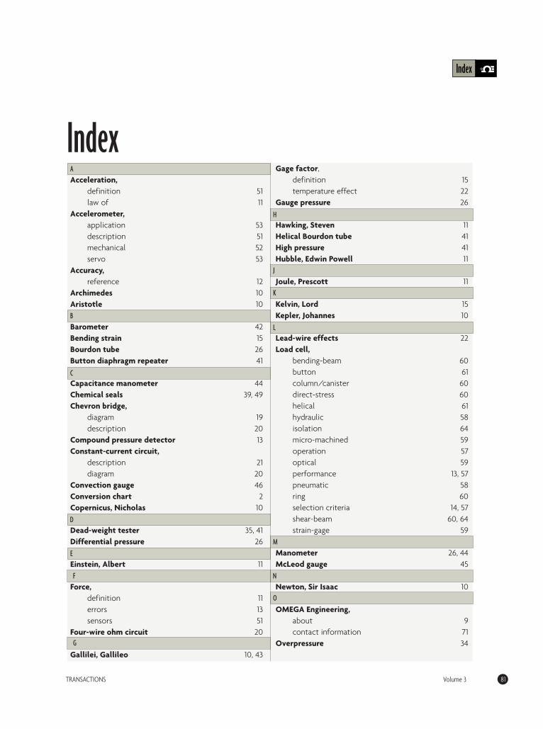
TRANSACTIONS Volume 3 81
Index
A
Index
B
C
D
E
G
Acceleration,definition 51law of 11
Accelerometer,application 53description 51mechanical 52servo 53
Accuracy,reference 12
Archimedes 10Aristotle 10
Barometer 42Bending strain 15Bourdon tube 26Button diaphragm repeater 41
Capacitance manometer 44Chemical seals 39, 49Chevron bridge,
diagram 19description 20
Compound pressure detector 13Constant-current circuit,
description 21diagram 20
Convection gauge 46Conversion chart 2Copernicus, Nicholas 10
Dead-weight tester 35, 41Differential pressure 26
Einstein, Albert 11
Force,definition 11errors 13sensors 51
Four-wire ohm circuit 20
Gallilei, Gallileo 10, 43
Gage factor,definition 15temperature effect 22
Gauge pressure 26
Hawking, Steven 11Helical Bourdon tube 41High pressure 41Hubble, Edwin Powell 11
Joule, Prescott 11
Kelvin, Lord 15Kepler, Johannes 10
Lead-wire effects 22Load cell,
bending-beam 60button 61column/canister 60direct-stress 60helical 61hydraulic 58isolation 64micro-machined 59operation 57optical 59performance 13, 57pneumatic 58ring 60selection criteria 14, 57shear-beam 60, 64strain-gage 59
Manometer 26, 44McLeod gauge 45
Newton, Sir Isaac 10
OMEGA Engineering,about 9contact information 71
Overpressure 34
F
H
J
K
L
M
N
O

Index
82 Volume 3 TRANSACTIONS
T
R
P
S
Pascal, Blaise 10Pirani gauge 45Pressure 12, 26Pressure gauge,
accessories 48, 49designs 48
Pressure switch,description 48design 50terminology 49
Pressure sensor,accessories 38calibration 37capacitance 29differential 29diaphragm designs 27electronic 27electrostatic 33inductive 34installation 38maintenance 37mechanical 27optical 35piezoelectric 31potentiometric 30resonant wire 31selection criteria 36strain gage 29
Ptolemaeus, Clausius 10Pulsation damper 36, 39
Rubbia, Carlo 11
Snubber 36, 39Stay rod 13Strain 15Strain gage,
application 21resistance wire 17, 18bridge circuits 3diffused seminconductor 18error 23guarding 21installation 21, 24sensor designs 16, 24shielding 21silicon 17stability 23
thin-film 17troubleshooting 24
Stress 15
Torque 54Torque sensor,
applications 54configurations 54inductive coupling 55magnetoelastic 56optical 55strain gage 55
Vacuum gaugesgauge designs 42applications 43cold-cathode 46hot-cathode 46ionization 46mechanical 44molecular momentum 45Pirani 45thermal 45thermocouple 45
Van der Meer, Simon 11Vibration
(see Acceleration)
Weighing system,application 62batching 68calibration 67design 63installation 67gain-in-weight 69loss-in-weight 69performance 63piping 66stabilization 65vessel support 64
Weight measurement,errors 13sensor configuration 60
Wheatstone bridge,compensation 58equations 19schematic 18
Wheatstone, Sir Charles 57
V
W

Index
TRANSACTIONS Volume 3 83
1-1. Steelyard for Weight Comparison 10
1-2. Vacuum Reference Gauge 11
1-3. Atmospheric Reference Gauge 11
1-4. Flexible Load-Cell Connections 12
1-5. Typical Load Cell Installation 12
1-6. Tank “Staying” Designs 13
2-1. Definitions of Stress & Strain 15
2-2. Shearing Strain 15
2-3. Poisson Strain 16
2-4. Strain Gage Designs 16
2-5. Bonded Resistance Strain Gage Construction 17
2-6. Wheatstone Bridge Circuit Schematic 18
2-7. Chevron Bridge Circuit Schematic 19
2-8. Four-Wire Ohm Circuit Schematic 20
2-9. Constant Current Circuit Schematic 20
2-10. Alternative Lead-Wire Configurations 21
2-11. Gage-Factor Temperature Dependence 22
2-12. Apparent Strain Variation with Temperature 23
2-13. Strain Gage Installation Alternatives 24
3-1. Bourdon Tube Designs 26
3-2. Pressure Sensitive Diaphragm Designs 27
3-3. Electronic Pressure Sensor Ranges 27
3-4. Strain-Gage Based Pressure Cell 28
3-5. Capacitance-Based Pressure Cell 28
3-6. Potentiometric Pressure Transducer 29
3-7. Resonant-Wire Pressure Transducer 30
3-8. Typical Piezoelectric Pressure Sensor 31
3-9. Acceleration-Compensated Piezoelectric Sensor 31
3-10. Magnetic Pressure Transducer Designs 32
3-11. Optical Pressure Transducer 33
3-12. Bourdon Tube Overpressure Protection 34
3-13. Three-Valve Manifold for
Instrumentation Isolation 35
3-14. Dead-Weight Tester Schematic 35
3-15. Pulsation Damper & Snubber Design 36
3-16. Chemical Seal Alternatives 37
3-17. Volumetric Seal Element Designs 38
4-1. Mechanical High Pressure Sensors 41
4-2. Bulk Modulus Cell 42
4-3. Barometer Operation 42
4-4. Vacuum Gauge Measurement Ranges 43
4-5. Manometer Designs 44
4-6. Capacitance Vacuum Manometer 45
4-7. Hot-Cathode Vacuum Gauge 46
4-8. Cold-Cathode Vaccum Gauge 46
5-1. Pressure Gauge Designs 48
5-2. Pressure Gauge Accessories 48
5-3. Pressure Switch Terminology 49
6-1. Piezoelectric Sensor Element Designs 51
6-2. Impact Flowmeter Application 52
6-3. Early Mechanical Vibration Sensor 53
6-4. Torque on a Rotating Shaft 54
6-5. Inductive Coupling of Torque Sensors 55
7-1. Load Cell Performance Comparison 57
7-2. Wheatstone Circuit with Compensation 58
7-3. Load Cell Spring Elements 59
8-1. Tank Staying Arrangement 62
8-2. Cantilever Load Cells
Reduce Staying Requirements 63
8-3. End-Loaded Shear-Beam Installation 64
8-4. Master Load Cell for Weighbridge Calibration 65
8-5. Treadle Scale Design 66
8-6. Monorail Weighing Transducer 67
8-7. Load Cell Configuration for Solids Batching 68
List of FiguresSection 1A Historical Perspective
Section 4High Pressure & Vacuum
Section 5Pressure Gauges & Switches
Section 6Force, Acceleration, & Torque
Section 7Load Cell Designs
Section 2The Strain Gage
Section 3Process Pressure Measurement
Section 8Weighing Applications

PLA
CE
STA
MP
HE
RE
PLA
CE
STA
MP
HE
RE
Com
plet
e Re
vers
e Si
de to
Rece
ive
Your
Ow
n
Dilb
ert C
ard
Deck
sO
ME
GA
EN
GIN
EE
RIN
G,I
NC
.O
NE
OM
EG
AD
RIV
EP.
O.B
OX
404
7S
TAM
FO
RD
CT
069
07-0
047
Com
plet
e Re
vers
e Si
de to
Rece
ive
Your
Ow
n
Hard
cove
r Han
dboo
ksO
ME
GA
EN
GIN
EE
RIN
G,I
NC
.O
NE
OM
EG
AD
RIV
EP.
O.B
OX
404
7S
TAM
FO
RD
CT
069
07-0
047 PLA
CE
STA
MP
HE
RE
PLA
CE
STA
MP
HE
RE
Com
plet
e Re
vers
e Si
de to
Rece
ive
Your
Ow
n
Gian
t Pos
ter B
ulle
tins!
OM
EG
AE
NG
INE
ER
ING
,IN
C.
ON
EO
ME
GA
DR
IVE
P.O
.BO
X 4
047
STA
MF
OR
D C
T 0
6907
-004
7
Com
plet
e Re
vers
e Si
de to
Rece
ive
Your
Ow
n
Tran
sact
ions
of
Mea
sure
men
t &Co
ntro
lO
ME
GA
EN
GIN
EE
RIN
G,I
NC
.O
NE
OM
EG
AD
RIV
EP.
O.B
OX
404
7S
TAM
FO
RD
CT
069
07-0
047

Fill out card completely. Please print inform
ation clearly:
Name
____________________________________________________Corporate e-m
ail:____________________________________________Personal e-m
ail:____________________________________________
Title______________________________________________________
Company
__________________________________________________Com
pany Address____________________________________________City__________________State______________Zip
________________Phone #
______________________Fax #
________________________If em
ployer does not permit handbook delivery at w
ork, give company address above
and home address below
. Catalogs cannot be delivered to P.O. Boxes.
Street Address________________________________________City
______________State__________Zip
______________
1. What is the principal activity at this location?
□ M
anufacturing□
Service□
R&D
2. What is the PRIM
ARY end product manufactured or service perform
edat your business location? (Please be specific):__________________________________________________________________________
3. What is the approxim
ate number of em
ployees at this location?□
1-19 □ 20-49 □
50-99 □ 100-499 □
500-999 □ 1000+
Already sent for your OMEGA
®Handbooks? Pass this card on. Your colleague w
ill thank you.©
COPYRIGHT 1998 OMEGA ENGINEERING, INC. ALL RIGHTS RESERVED.
YES!Send M
e the Following
BRAND NEW!, FREE!
OMEGA
®Handbook(s).
MP
urchasing Ag
ent Edition
MTem
perature and Hum
idityM
Pressure
,Strain,
and Force
MF
low
and Level
MpH
and Conductivity
MD
ata Acquisition H
andbookM
Universal G
uide to D
ata Acquisition
ME
lectric Heater
sM
The G
reen Book
®
M21
STC
enturyTM
Previe
w E
ditionM
Book of B
ooks®
Update
MTransactions
From
our affiliate companies
MO
ME
GA
DY
NE
TM P
ressureForce Load Torque D
atabook M
NE
WP
OR
T®Volum
e V D
atabook
Fill out card completely. Please print inform
ation clearly:
Name______________________________________________________
Corporate e-mail:____________________________________________
Personal e-mail:
____________________________________________
Title______________________________________________________
Company
__________________________________________________
Company Address____________________________________________
City__________________State______________Zip________________
Phone #______________________
Fax #________________________
If employer does not perm
it handbook delivery at work, give com
pany address aboveand hom
e address below. Catalogs cannot be delivered to P.O. Boxes.
Street Address________________________________________
City______________State
__________Zip______________
1. What is the principal activity at this location?
□ M
anufacturing□
Service□
R&D
2. What is the PRIM
ARY end product manufactured or service perform
edat your business location? (Please be specific):__________________________________________________________________________
3. What is the approxim
ate number of em
ployees at this location?□
1-19 □ 20-49 □
50-99 □ 100-499 □
500-999 □ 1000+
YES!Send M
e the BRAND NEW!,
FREE! Dilbert Deck Cards!M
Dilbert D
eck Cards
YES!Send M
e the Following
BRAND NEW!, FREE!
OMEGA
®Transactions of
Measurem
ent andControl:
MInfrared
Temperature
Measurem
ent andC
ontrol (1Q98)
MD
ata Acqusition in
Process C
ontrol (2Q
98)
MP
ressure,F
orce,and
Load Measurem
ent and C
ontrol
(3Q98)
MM
easurement and
Control of E
nvironm
entalP
arameters (4Q
98)
Fill out card completely. Please print inform
ation clearly:
Name______________________________________________________
Corporate e-mail:____________________________________________
Personal e-mail:
____________________________________________
Title______________________________________________________
Company
__________________________________________________
Company Address____________________________________________
City__________________State______________Zip________________
Phone #______________________
Fax #________________________
If employer does not perm
it handbook delivery at work, give com
pany address aboveand hom
e address below. Catalogs cannot be delivered to P.O. Boxes.
Street Address________________________________________
City______________State
__________Zip______________
1. What is the principal activity at this location?
□ M
anufacturing□
Service□
R&D
2. What is the PRIM
ARY end product manufactured or service perform
edat your business location? (Please be specific):__________________________________________________________________________
3. What is the approxim
ate number of em
ployees at this location?□
1-19 □ 20-49 □
50-99 □ 100-499 □
500-999 □ 1000+
YES!Send M
e the Following
BRAND NEW!, FREE!
OMEGA
®Giant Posters:
MS
pace Shuttle
Patc
hes
MR
ockets of the W
orld
MC
hart ofD
imensionless
Num
bers
MR
adio Frequencies
MD
ilbert Deck
Dilbert ©
United F
eature Syndicate, Inc.
Fill out card completely. Please print inform
ation clearly:
Name
____________________________________________________
Corporate e-mail:____________________________________________
Personal e-mail:
____________________________________________
Title______________________________________________________
Company
__________________________________________________
Company Address____________________________________________
City__________________State______________Zip________________
Phone #______________________
Fax #________________________
If employer does not perm
it handbook delivery at work, give com
pany address aboveand hom
e address below. Catalogs cannot be delivered to P.O. Boxes.
Street Address________________________________________City
______________State__________Zip
______________
1. What is the principal activity at this location?
□ M
anufacturing□
Service□
R&D
2. What is the PRIM
ARY end product manufactured or service perform
edat your business location? (Please be specific):__________________________________________________________________________
3. What is the approxim
ate number of em
ployees at this location?□
1-19 □ 20-49 □
50-99 □ 100-499 □
500-999 □ 1000+
Already sent for your Dilbert DeckCards? Pass this card on. Your colleague w
ill thank you.©
COPYRIGHT 1998 OMEGA ENGINEERING, INC.
ALL RIGHTS RESERVED.
Already sent for your OMEGA
®Giant
Poster Bulletins? Pass this card on.Your colleague w
ill thank you.©
COPYRIGHT 1998 OMEGA ENGINEERING, INC.
ALL RIGHTS RESERVED.
Already sent for your OMEGA
®Transactions
of Measurem
ent and Control? Pass thiscard on. Your colleague w
ill thank you.©
COPYRIGHT 1998 OMEGA ENGINEERING, INC.
ALL RIGHTS RESERVED.

omega.comomega.com®®
®®