Setting SpecificationsStatistical considerations

Enda Moran – Senior Director, Development, PfizerMelvyn Perry – Manager, Statistics, Pfizer

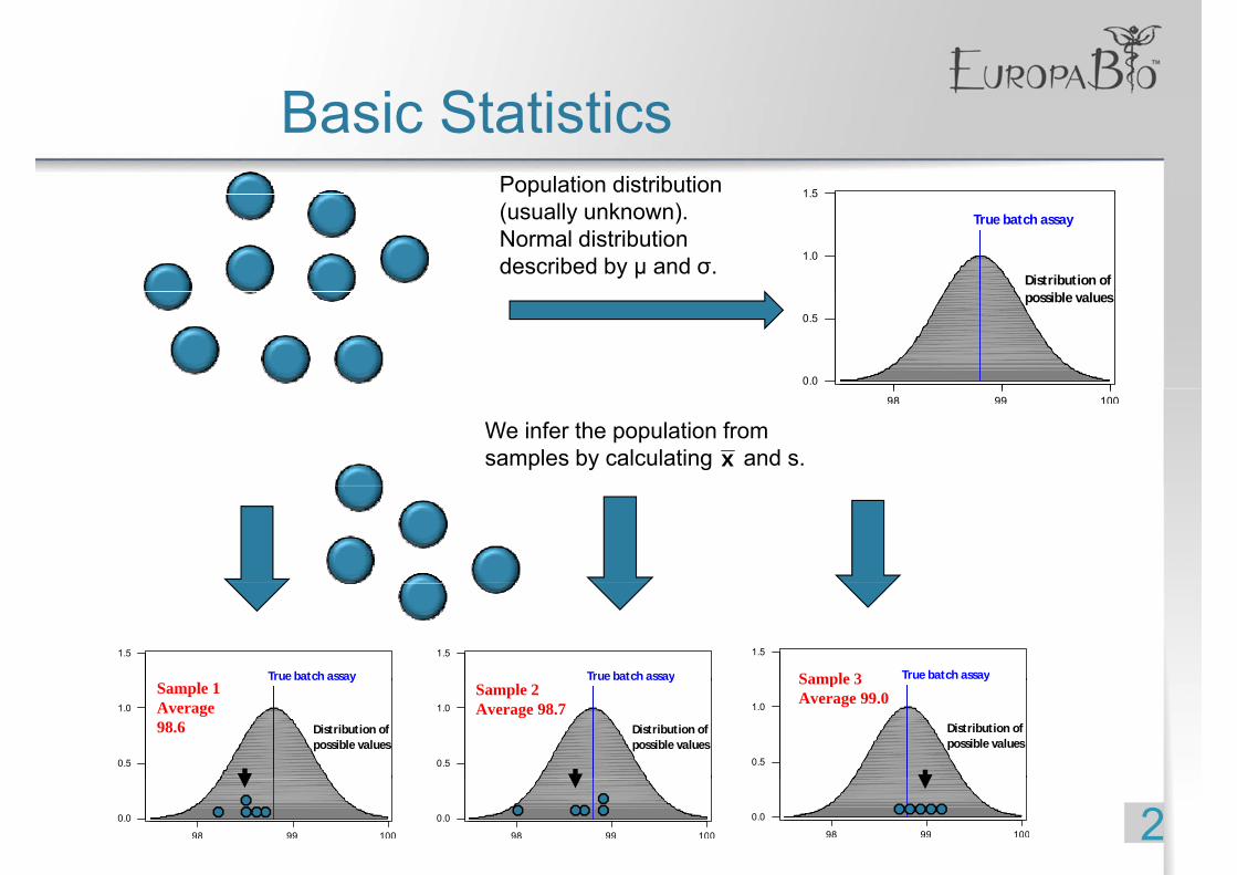
B i St ti tiBasic Statistics1 5Population distribution 1.5

1.0

True batch assay

Distribution of

p(usually unknown).Normal distribution described by μ and σ.

0.5

0.0

possible values

1009998

We infer the population from samples by calculating and s.x

1.5

True batch assay

1.5

True batch assay

1.5

True batch assaySample 3

1.0

0.5

y

possible valuesDistribution of

Sample 1 Average 98.6

1.0

0.5

y

possible valuesDistribution of

Sample 2 Average 98.7 1.0

0.5

y

possible valuesDistribution of

Sample 3 Average 99.0

21009998

0.0

1009998

0.0

1009998

0.0

I t lIntervals30

28

30

24

26

22

Populationaverage

18

20

0 10 20 30 40 50 60 70 80 90 10016

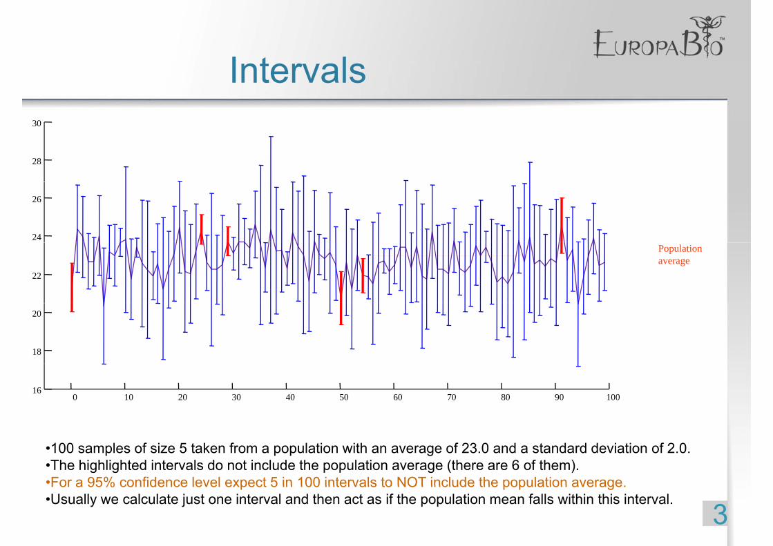
•100 samples of size 5 taken from a population with an average of 23.0 and a standard deviation of 2.0.•The highlighted intervals do not include the population average (there are 6 of them).•For a 95% confidence level expect 5 in 100 intervals to NOT include the population average

3For a 95% confidence level expect 5 in 100 intervals to NOT include the population average.

•Usually we calculate just one interval and then act as if the population mean falls within this interval.

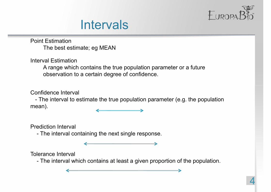
I t lIntervalsPoint EstimationPoint Estimation

The best estimate; eg MEAN

Interval EstimationA range which contains the true population parameter or a future observation to a certain degree of confidence.

Confidence Interval- The interval to estimate the true population parameter (e.g. the population

mean)mean).

Prediction IntervalPrediction Interval- The interval containing the next single response.

Tolerance Interval- The interval which contains at least a given proportion of the population.

4

F l f I t lFormulae for Intervals

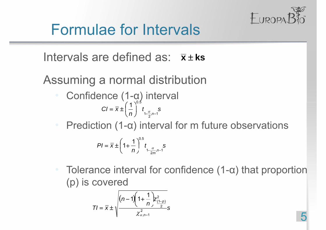
Intervals are defined as:

A i l di t ib ti

ksx ±

Assuming a normal distribution• Confidence (1-α) interval

50⎞⎛

• Prediction (1-α) interval for m future observations

stn

xCIn 1,

21

5.01−−

⎟⎠⎞

⎜⎝⎛±= α

Prediction (1 α) interval for m future observations

stn

xPIn

m1,

21

5.011−−

⎟⎠⎞

⎜⎝⎛ +±= α

• Tolerance interval for confidence (1-α) that proportion ( ) i d

m2⎠⎝

(p) is covered( ) z

nn p

2)1(

111 −⎟⎠⎞

⎜⎝⎛ +−

5s

nxTI

n2

1,

2

−

⎠⎝±=αχ

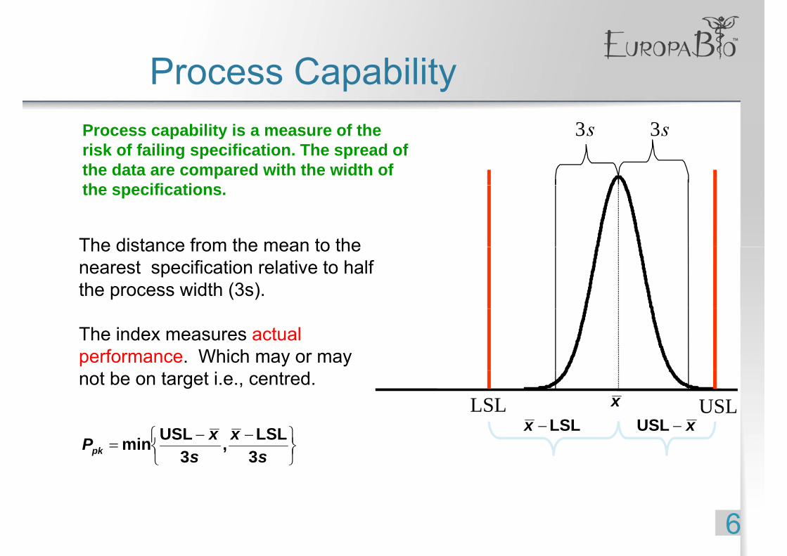
P C bilitProcess Capability33 s3s3Process capability is a measure of the

risk of failing specification. The spread of the data are compared with the width of th ifi ti

The distance from the mean to the

the specifications.

The distance from the mean to the nearest specification relative to half the process width (3s).

The index measures actual performance. Which may or may not be on target i.e., centred.

⎫⎧ xx LSLUSLUSLLSL x

LSL−x x−USL

⎭⎬⎫

⎩⎨⎧ −−

=s

xs

xPpk 3LSL,

3USLmin

6

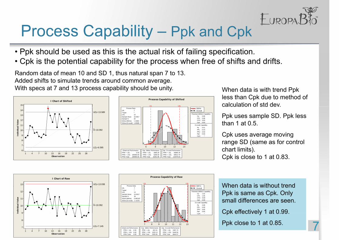
P C bilit P k d C kProcess Capability – Ppk and Cpk• Ppk should be used as this is the actual risk of failing specification

Random data of mean 10 and SD 1, thus natural span 7 to 13.Added shifts to simulate trends around common average

Ppk should be used as this is the actual risk of failing specification. • Cpk is the potential capability for the process when free of shifts and drifts.

LSL USL

Process Capability of Shifted

151

I Chart of Shifted

Added shifts to simulate trends around common average.With specs at 7 and 13 process capability should be unity. When data is with trend Ppk

less than Cpk due to method of calculation of std dev.

LSL 7Target *USL 13Sample Mean 10.0917Sample N 30StDev (Within) 1.16561StDev (O v erall) 1.95585

Process Data

C p 0.86C PL 0.88C PU 0.83C pk 0.83

Pp 0.51PPL 0.53PPU 0.50

O v erall C apability

Potential (Within) C apability

WithinOverall14

13

12

11

10

divi

dual

Val

ue

_X=10.092

UCL=13.589

1 calculation of std dev.

Ppk uses sample SD. Ppk less than 1 at 0.5.

C k i

14121086

Ppk 0.50C pm *

PPM < LSL 0.00PPM > USL 100000.00PPM Total 100000.00

O bserv ed PerformancePPM < LSL 3995.30PPM > USL 6296.59PPM Total 10291.88

Exp. Within PerformancePPM < LSL 56966.34PPM > USL 68512.70PPM Total 125479.03

Exp. O v erall Performance

28252219161310741

9

8

7

6

Observation

Ind

LCL=6.595

Cpk uses average moving range SD (same as for control chart limits).Cpk is close to 1 at 0.83.

13 UCL=13.038

I Chart of Raw

LSL USLProcess Data Within

Process Capability of Raw

p

When data is without trend12

11

10

9Indi

vidu

al V

alue

_X=10.092

LSL 7Target *USL 13Sample Mean 10.0917Sample N 30StDev (Within) 0.982187StDev (O v erall) 1.14225

C p 1.02C PL 1.05C PU 0.99C pk 0.99

Pp 0.88PPL 0.90PPU 0.85Ppk 0.85C *

O v erall C apability

Potential (Within) C apability

OverallWhen data is without trend Ppk is same as Cpk. Only small differences are seen.

Cpk effectively 1 at 0.99.

728252219161310741

9

8

7

Observation

I

LCL=7.14513121110987

C pm *

PPM < LSL 0.00PPM > USL 0.00PPM Total 0.00

O bserv ed PerformancePPM < LSL 822.51PPM > USL 1533.13PPM Total 2355.65

Exp. Within PerformancePPM < LSL 3397.73PPM > USL 5446.84PPM Total 8844.57

Exp. O v erall Performance

Cpk effectively 1 at 0.99.

Ppk close to 1 at 0.85.

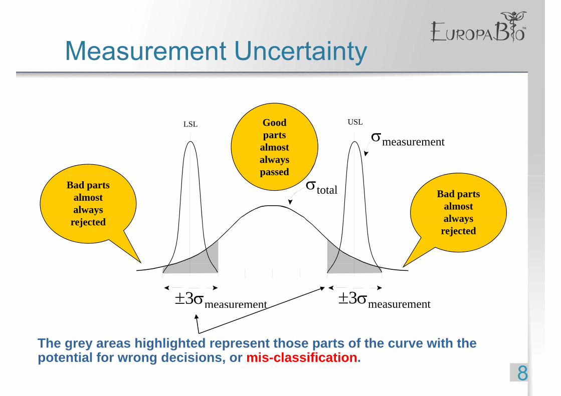
M t U t i tMeasurement Uncertainty

Goodt

LSL USL

parts almost always passed

σmeasurement

pBad parts

almost always

j t d

Bad parts almost always

σtotal

rejected always rejected

±3σmeasurement ±3σmeasurement

The grey areas highlighted represent those parts of the curve with the

8potential for wrong decisions, or mis-classification.

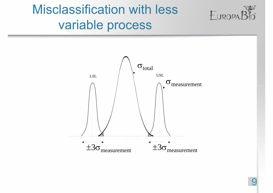
Misclassification with less i blvariable process

σLSL USL

σmeasurement

σtotal

measurement

±3σmeasurement ±3σmeasurement3σmeasurement measurement

9

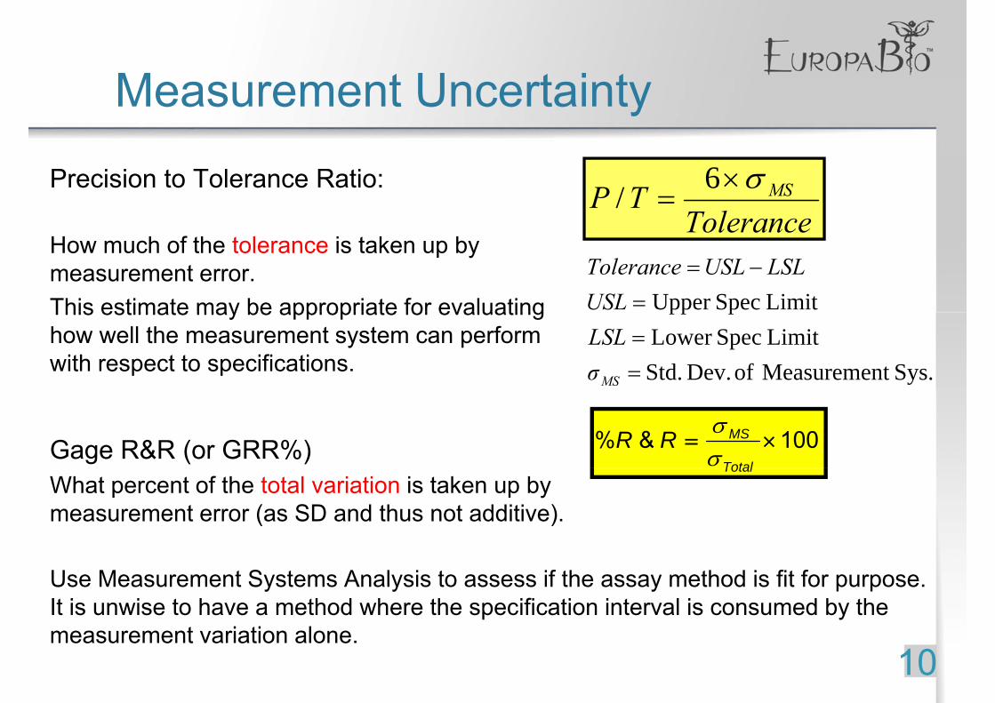
M t U t i tMeasurement Uncertainty

Precision to Tolerance Ratio:

ToleranceTP MSσ×=

6/How much of the tolerance is taken up bymeasurement error.This estimate may be appropriate for evaluating LimitSpecUpper =

−=USL

LSLUSLTolerance

This estimate may be appropriate for evaluatinghow well the measurement system can performwith respect to specifications. Sys.t Measuremen of Dev. Std.

Limit SpecLower ppp

==

MSσLSL

Gage R&R (or GRR%) 100&% ×=Total

MSRRσσ

What percent of the total variation is taken up bymeasurement error (as SD and thus not additive).

Total

Use Measurement Systems Analysis to assess if the assay method is fit for purpose. It is unwise to have a method where the specification interval is consumed by the

10measurement variation alone.

Specification example –T l I t lTolerance Interval

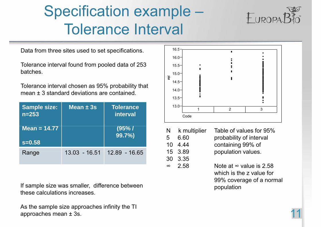
16.5Data from three sites used to set specifications

15.0

15.5

16.0

16.5Data from three sites used to set specifications.

Tolerance interval found from pooled data of 253 batches.

13.5

14.0

14.5Tolerance interval chosen as 95% probability that mean ± 3 standard deviations are contained.

13.01 2 3

Code

Sample size: n=253

Mean ± 3s Toleranceinterval

( % / N k multiplier5 6.6010 4.4415 3 89

Table of values for 95% probability of interval containing 99% of population values

Mean = 14.77

s=0.58

(95% / 99.7%)

R 13 03 16 51 12 89 16 65 15 3.8930 3.35∞ 2.58

population values.

Note at ∞ value is 2.58 which is the z value for

Range 13.03 - 16.51 12.89 - 16.65

99% coverage of a normal populationIf sample size was smaller, difference between

these calculations increases.

11As the sample size approaches infinity the TI approaches mean ± 3s.

Specification Example -St bilitStability

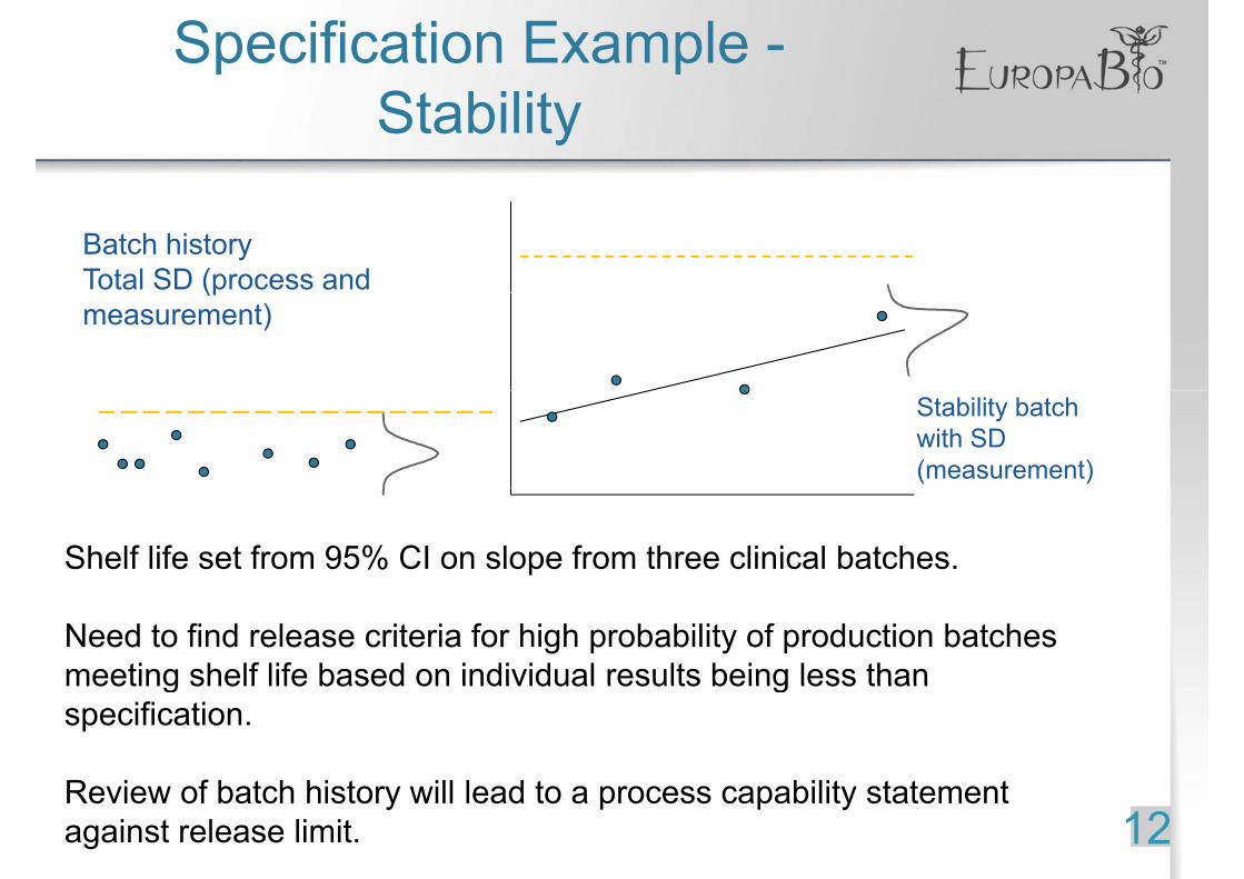
Batch historyTotal SD (process and (pmeasurement)

Stability batch with SD (measurement)

Shelf life set from 95% CI on slope from three clinical batches.

Need to find release criteria for high probability of production batches meeting shelf life based on individual results being less thanmeeting shelf life based on individual results being less than specification.

R i f b t h hi t ill l d t bilit t t t12

Review of batch history will lead to a process capability statement against release limit.

Specification Example -St bilitStability

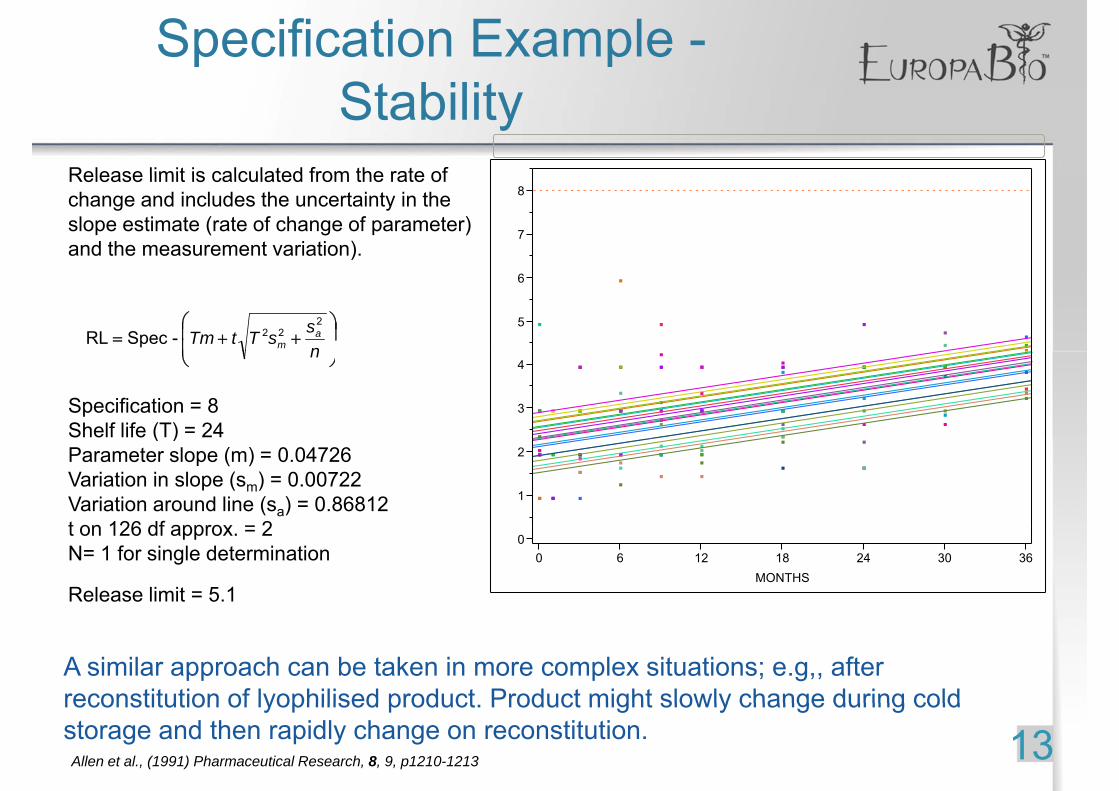
Release limit is calculated from the rate of

7

8Release limit is calculated from the rate of change and includes the uncertainty in the slope estimate (rate of change of parameter) and the measurement variation).

5

6

⎟⎟⎠

⎞⎜⎜⎝

⎛++=

nssTtTm a

m

222 -Spec RL

3

4⎟⎠

⎜⎝ n

Specification = 8Shelf life (T) = 24

1

2( )

Parameter slope (m) = 0.04726Variation in slope (sm) = 0.00722Variation around line (sa) = 0.86812t on 126 df approx = 2 0

0 6 12 18 24 30 36MONTHS

t on 126 df approx. = 2N= 1 for single determination

Release limit = 5.1

A similar approach can be taken in more complex situations; e.g,, after reconstitution of lyophilised product Product might slowly change during cold

13reconstitution of lyophilised product. Product might slowly change during cold storage and then rapidly change on reconstitution.Allen et al., (1991) Pharmaceutical Research, 8, 9, p1210-1213

C i ith li it d d tCoping with limited dataProblems with n<30.

• Difficult to calculate a reliable estimate of the SD.• Difficult to assess distribution.Difficult to assess distribution.• Difficult to assess process stability.

With very limited data the specifications will be wide due to the large multiplierWith very limited data the specifications will be wide due to the large multiplier.• This reflects the uncertainty in the estimates of the mean and SD.

Is there a small scale model that matches full production scale?Is there a small scale model that matches full production scale?

How variable is the measurement system?

Alternatives are:• Min / max values based on

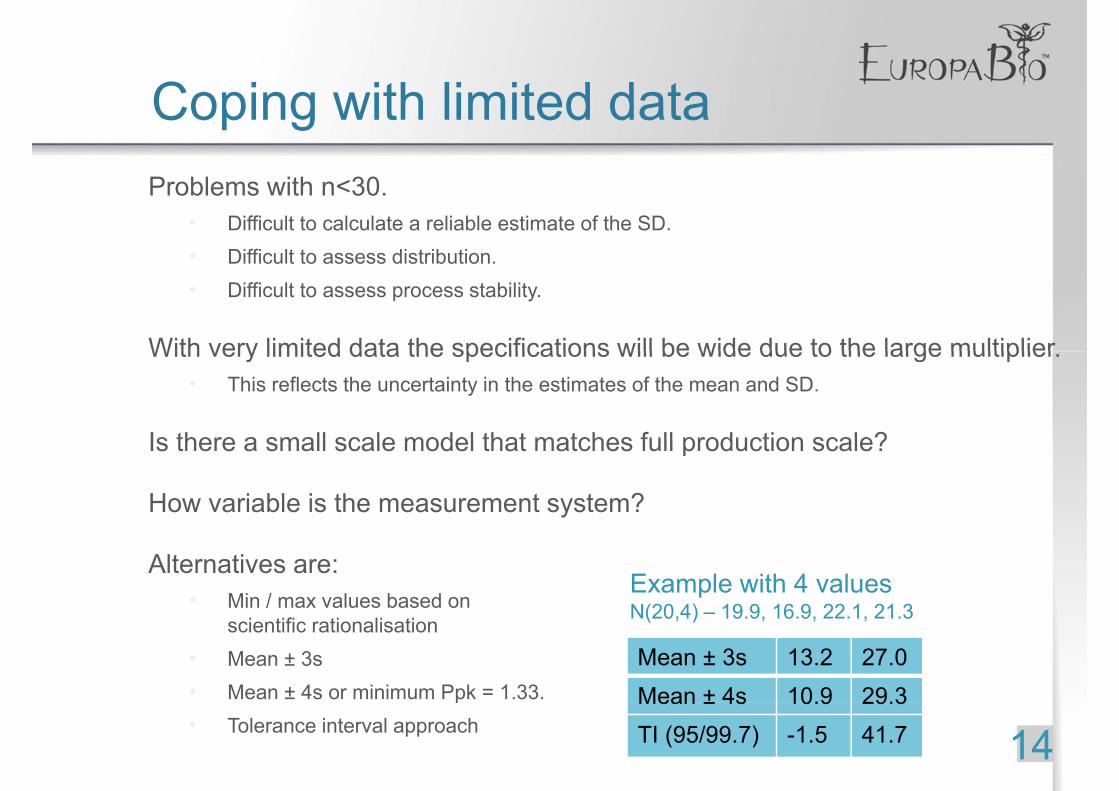
Example with 4 valuesN(20 4) – 19 9 16 9 22 1 21 3

scientific rationalisation• Mean ± 3s• Mean ± 4s or minimum Ppk = 1.33.

Mean ± 3s 13.2 27.0Mean ± 4s 10.9 29.3

N(20,4) 19.9, 16.9, 22.1, 21.3

p• Tolerance interval approach 14

Mean ± 4s 10.9 29.3TI (95/99.7) -1.5 41.7

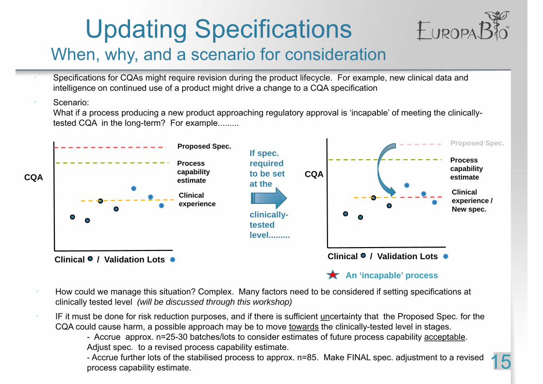
Updating Specifications

• Specifications for CQAs might require revision during the product lifecycle. For example, new clinical data and i t lli ti d f d t i ht d i h t CQA ifi ti

p g pWhen, why, and a scenario for consideration

intelligence on continued use of a product might drive a change to a CQA specification

• Scenario: What if a process producing a new product approaching regulatory approval is ‘incapable’ of meeting the clinically-tested CQA in the long-term? For example.........

Proposed Spec.

Process capability

If spec. required t b t

Proposed Spec.

Process capability

CQA

Clinical experience

capability estimate

to be set at the

clinically

CQA

Clinical experience / New spec.

capability estimate

clinically-tested level.........

Clinical / Validation LotsClinical / Validation Lots Clinical / Validation Lots

An ‘incapable’ process

• How could we manage this situation? Complex. Many factors need to be considered if setting specifications at ( )clinically tested level (will be discussed through this workshop)

• IF it must be done for risk reduction purposes, and if there is sufficient uncertainty that the Proposed Spec. for the CQA could cause harm, a possible approach may be to move towards the clinically-tested level in stages.

- Accrue approx. n=25-30 batches/lots to consider estimates of future process capability acceptable.

15pp p p y p

Adjust spec. to a revised process capability estimate.- Accrue further lots of the stabilised process to approx. n=85. Make FINAL spec. adjustment to a revised process capability estimate.

SSummary

• Process capability & measurement uncertainty

• Setting spec.s - large number of datapoints

• Setting spec.s – small number of datapoints

16