Precise Structural Vulnerability Assessment via Mathematical Programming

Outline Introduction Sparse Metric Branch & Cut Method Experimental Analysis Conclusion

Precise Structural Vulnerability Assessment viaMathematical Programming

Thang N. Dinh and My T. Thai

Department of Computer & Information Science & EngineeringUniversity of Florida, Gainesville, FL 32611

November 09, 2011


1 IntroductionPairwise-connectivity and β-disrutpor

2 Sparse MetricLinear ProgrammingSparse Metric

3 Branch & Cut MethodCutting PlanePrimal Heuristic

4 Experimental AnalysisSynthetic NetworksCase study: Western Power Grid

5 Conclusion


Vulnerability of Network Systems

Many networks are vulnerable to both natural disaster andintentional attacks

Failures of network infrastructure, nodes or links, lead todisruption of services.

Example:

Earthquake near Taiwan disrupts Internet trafficAnchor cut undersea fiber-opticTerrorism activities targeting highway system


Network Vulnerability Assessment

Assessing the fatal failure schemes before they happen isessential

Disaster recovery planHardening critical infrastructureReduce the worst case impact

Finding the most critical nodes and links that failures willseverly disrupt the network

How to measure the impact of the failures?

The connectivity level in the residual network: The number ofconnected pairs a.k.a. pairwise connectivity.


Vulnerability Assessment as an Optimization Problem

Given a network modeled by a graph G = (V ,E ), aβ-vertex disruptor is a set of vertices that removal lessen thepairwise connectivity to no more than β

(|V |2

).

Smaller the size of β-vertex disruptors, the more vulnerablethe network is

Compute the minimum size of a beta-vertex disruptor as anindex to measure the network vulnerablity

We can define β-edge disruptor in the same manor.


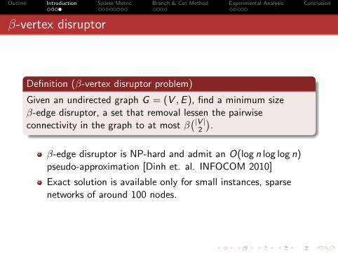
β-vertex disruptor

Definition (β-vertex disruptor problem)

Given an undirected graph G = (V ,E ), find a minimum sizeβ-edge disruptor, a set that removal lessen the pairwiseconnectivity in the graph to at most β

(|V |2

).

β-edge disruptor is NP-hard and admit an O(log n log log n)pseudo-approximation [Dinh et. al. INFOCOM 2010]

Exact solution is available only for small instances, sparsenetworks of around 100 nodes.


Linear Integer Programming (IP)

minimizen∑

i=1

si (1)

subject to dij ≤ si + sj , (i , j) ∈ E , (2)

dij + djk ≥ dik , ∀i 6= j 6= k (3)∑

i<j

dij ≥ (1− β)

(n

2

), (4)

si ≤ dij , i 6= j (5)

si , dij ∈ {0, 1}, i , j ∈ [1..n] (6)

dij =

{0 if i and j are connected1 otherwise.

si =

{0 if node i is not removed1 if i is removed.


Linear Integer Programming (cont.)

IP has 13n × (n − 1)× (n − 2) = θ(n3) constraints!!!

The number of integral variables n +(n

2

)= θ(n2).

Require excessive amount of memory and processing time.

Largest solved instances have around 100 nodes.

Denote the LP relaxation in which 0 ≤ si , dij ≤ 1 by LP(large)


Mixed Integer Programming

Replace si , dij ∈ {0, 1} by si ∈ {0, 1}, 0 ≤ dij ≤ 1.

Only n integral variables si .

Equivalent to the IP.

It still has θ(n3) constraints.

Lemma

The MIP and IP have the same set of optimal basic solutions.


Sparse Metric

The constraint dij + djk ≥ dik is equivalent to saying that dijis a (semi) metric.

Not all constraints dij + djk ≥ dik are tight at the optimalsolutions (for both IP and LP)

Remove those unnessary (non-binding) constraints can reduceboth time and memory requirements.

Which constraints to keep/remove?


Sparse Metric (cont.)

A new compact Mixed Integer Programming, called MIP(Sparse):

dij + djk ≥ dik , k ∈ [1..n]→ dij + djk ≥ dik , k ∈ Nmin(i , j)

Nmin(i , j) = N(i) if d(i) < d(j), and N(j) otherwise.

There are at most O(mn) constraints that is O(n2) for manynetworks of interests

#constraints = |E |+∑

i<j

min {d(i), d(j)}+n(n − 1)

2

≤n2 +∑

i<j

d(i) + d(j)

2= n2 +

n − 1

2

n∑

i=1

d(i) = O(mn)

Denote the LP relaxation in which dij ∈ [0, 1] by LP(sparse)



Both the integer programming and the relaxation of the sparsemetric are equivalent to those of the original formula.



Theorem

The MIP (sparse) and the IP (large) have the same set of optimalsolutions.

Proof.Round all dij > 0 to 1. This will not violate constraints (5) and (4). For constraints (2), if dij is rounded up to 1then the integrality of si , sj implies si + sj ≥ 1, or else if dij = 0 then the constraints are still satisfied. Assumethe rounding violates constraints (3) for some triple (i, j, k). This happens if and only if dik = 1 anddij = djk = 0. Hence, before rounding, dik > 0 and dij = dj,k = 0 that contradicts the constraintdij + djk ≥ dik . It follows that rounding gives a feasible integral solution to the MIP.For each connected pair (i, j) in G[V\DMIP ], we prove that dij = 0 by induction on the length t of the shortest

path (in number of hops) between nodes i and j .The basis. The statement holds for t = 1. By constraint (2), if (i, j) ∈ E and i, j are connected in G i.e.si = sj = 0, then dij ≤ si + sj = 0. Since dij ≥ 0, it follows that dij = 0.

The inductive step. Assume that the statement holds for t = t′, we show that the statement is also true for

t = t′ + 1. Let i, j be some pairs connected with a path of length at most t′ + 1. Since removing all nodes in

Nmin(i, j) disconnects i from j , the path between i and j must pass through some node k ∈ Nmin(i, j). In

addition, the shortest paths from i to k and from k to j have lengths at most t′. Thus, by the induction hypothesis

we have dik = dkj = 0. It follows from the constraint in (3) that dij ≤ dik + dkj = 0. Thus, the statement holds

for all t > 0.



Theorem

The LP (sparse) and the LP (large) have the same set of optimalbasic solutions.

Proof.Let (s, d) be an optimal fraction solution of the LP relaxation of MIPvd. Associate a weight dij for each edge

(i, j) ∈ E . Let d′ij be the shortest distance between two nodes (i, j) with the new edge weights. We have

1 d′ij ≥ dij for all i, j and d′ij = dij∀(i, j) ∈ E .

2 d′ij = minnk=1{d′ik + d′kj}. Hence, d′ij is a pseudo-metric.

The first statement can be shown by the same induction in the previous proof. The second statement comes fromthe definition of d′ij .Furthermore, we define d∗ij = min{d′ij , 1}. By definition, we have d∗ij = min{d′ij , 1} ≥ min{dij , 1} = dij ∀i, jand d∗ij = dij ∀(i, j) ∈ E . Thus, for all (i, j) ∈ E , d∗ij = dij ≤ si + sj . In addition, d∗ is also a pseudo-metric as

d∗ik + d∗kj ≥ min{d′ik + d′kj , 1} ≥ min{d′ij , 1} = d∗ij . From d∗ij ≥ dij , we have∑i,j

d∗i,j ≥∑i,j

di,j ≥ β(n

2

)and

si ≤ dij ≤ d∗ij . Thus, (s, d∗) is a solution of IP(large).

Obviously, the minimum objective of the LP relaxation of MIP(sparse) is smaller or equal to that of IP(large).

Since, the objective values associate with (s, d∗) and (s, d) are the same, (s, d∗) must be a minimum solution of

the LP relaxation of IP(large).


Branch & Cut Method

A generalization of branch-and-bound, an efficient method tosolve exactly many combinatorial optimization problems.

After solving the LP relaxation, try to find a violated cut.

If some violated cuts are found, we add them to theformulation and solve the LP again

If none are found, we branch.


Vertex-Cut

A subset S ⊂ V is a vertex-cut for a pair (u, v), if removing Sfrom graph G , disconnect s and t.

For all vertex-cut S of (u, v), if∑

i∈S si = |S |, then duv mustbe one. Thus, we have the VC inequality

∑

i∈Ssi − duv ≤ |S | − 1


Separation Procedure

A separation procedure finds a violated cut if any or return nosuch cut exists.

Solve the maximum-flow (min-cut) problem in networks withboth node and edge capacities.

Obviously, the minimum objective of the LP relaxation ofMIPvd is smaller or equal to that of IPvd. Since, the objectivevalues associate with (s, d∗) and (s, d), a minimum solutionof the LP relaxation of MIPvd, are the same, (s, d∗) must bea minimum solution of the LP relaxation of IPvd.

B. Cutting Planes

We present a class of strong cutting planes together with theseparation procedure to identify those cutting planes. Thesecan be used in conjunction with cutting planes generatedautomatically by optimization packages to improve the con-vergence of the branch-and-cut algorithm.

1) Vertex-Connectivity and Invalid Inequalities: One of-ten overlooked characteristic of solutions for clustering andpartitioning problems on graph is that clusters must induceconnected subgraph. This characteristic is not reflected ineither IPvd or MIPvd formulations.

A subset S ⊂ V is a vertex-cut for a pair (u, v), if removingS from graph G, disconnect s and t. For all vertex-cut S of(u, v), if

∑i∈S si = |S|, then duv must be one. Thus, we have

VC inequality ∑

i∈Ssi − duv ≤ |S| − 1

This inequality is valid for all feasible points inside thepolyhedra of MIPvd.

Algorithm 1. Separation procedure for VC inequalities

1: for each pair (u, v) ∈ V × V do2: Construct a flow network G = (V,E) as follows3: Assign u and v as source and sink, respectively4: Each node k ∈ V has capacity sk5: Every edge has capacity ∞6: if (u, v) ∈ E, then (u, v) has capacity zero.7: Find the maximum-flow (min-cut)8: if maximum-flow is less than duv , then9: Find the min vertex-cut S

10: Add the VC inequality associated with S to MIP8: end if

11: end for

2) Separation Procedure for VC Inequalities: Given a point(fractional solution) (s, d) ∈ R(n+1

2 ), an exact separationalgorithm for some class of inequalities either finds a memberof the class violated by (s, d), or proves that no such memberexists. In many cases, finding such algorithm is intractable(NP-hard problem) and one has to settle for heuristic pro-cedures. Fortunately, there is an exact algorithm for ourseparation procedure based on finding the max-flow on thenetwork with node capacities.

The VC inequality can be rewritten as∑

i∈Ssi − duv ≥ 0, S is any vertex-cut of (u, v)

where si = 1− si and duv = 1− duv .Therefore, the point (s, d) violates this inequality if and

only if∑i∈S si < duv . The most violated inequality is the

Algorithm 2. Sharpest Decreasing Vertices (SDV)

1: Start with some β-vertex disruptor D ⊆ V .2: Repeat3: while (true) do4: u = arg min

v∈D{P(G[V \(D∪{v})])}

5: if (D \ {u} is a β-disruptor) then D = D \ {u}6: for each (w ∈ V \ D) do7: Dw = D ∪ {w}8: u = arg min

v∈D{P(G[V \(Dw∪{v})])}

9: +if (u 6= w) then D = Dw ∪ {u}10: Until (D not changing)11: Output D.

one that minimize the sum∑i∈S si, given S is a vertex-

cut of (u, v). Thus, the subset S corresponding to the mostviolated inequalities can be found using minimum capacitatedvertex-cut of (u, v). The separation procedure is described inAlgorithm 1. Here, we need to solve the maximum-flow (min-cut) problem in networks with both node and edge capacities.If we apply Push-relabel algorithm with dynamic trees [?],the time complexity to find cutting planes for one node pair isO(mn log n2

m ). The total time complexity for the separationprocedure will be O(n3m log n2

m ). In our implementation,this procedure is called sparingly in order to avoid excessiverunning time.

C. Primal Heuristic

The search for an optimal solution in a branch and cutalgorithm can be accelerated by obtaining a high qualityfeasible solution to provide upper bounds for pruning othersubproblems. We present a heuristic that rounds the fractionalsolution of MIP relaxations to get integral solutions.

Let (s, d) be a fractional solution of an LP relaxation. Wefirst sort si in non-decreasing order si1 ≤ si2 ≤ . . . ≤ sin .Then we round down all si1 , si2 , . . . , sik to zero and round upsik+1

, sik+2, . . . , sin to one, where k runs from 1 to n. If the

obtain solution is a β-vertex disruptor, a local search methoddescribed in Algorithm 2 is then used to refine the solution.The local search method refines the solution by repeatedly:

• Removing node(s) from the disruptor if possible• Swapping a node w outside the disruptor with a nodeu in the disruptor that gives the sharpest decrease inconnectivity.

The local search terminates when no improvement exists.

IV. COMPUTATIONAL EXPERIMENTS

We implement our branch and cut algorithm using GUROBI4.0 on a computer with Intel Xeon 2.93 Ghz processor and12 GB memory. Table I shows results for IPvd and our newbranch and cut algorithm (MIPvd) on power-law networks [?]of various sizes. We report for each disruption level β, thenumber of removed vertices in the optimal solution, the num-ber of Rows (constraints), Nonzeros (nonzero coefficients),and solving time.


Primal-heuristic

Provide upper bounds for pruning subproblems

Let (s, d) be a fractional solution of the LP.

Sort si in non-decreasing order si1 ≤ si2 ≤ . . . ≤ sin .

Round down all si1 , si2 , . . . , sik to zero and round upsik+1

, sik+2, . . . , sin to one, where k runs from 1 to n.

If the obtain solution is a β-vertex disruptor, a local searchmethod is then used to refine the solution.


Primal-heuristic (cont.)

The local search method refines the solution by repeatedly:

Removing node(s) from the disruptor if possible

Swapping a node w outside the disruptor with a node u in thedisruptor that gives the sharpest decrease in connectivity.

Obviously, the minimum objective of the LP relaxation ofMIPvd is smaller or equal to that of IPvd. Since, the objectivevalues associate with (s, d∗) and (s, d), a minimum solutionof the LP relaxation of MIPvd, are the same, (s, d∗) must bea minimum solution of the LP relaxation of IPvd.

B. Cutting Planes

We present a class of strong cutting planes together with theseparation procedure to identify those cutting planes. Thesecan be used in conjunction with cutting planes generatedautomatically by optimization packages to improve the con-vergence of the branch-and-cut algorithm.

1) Vertex-Connectivity and Invalid Inequalities: One of-ten overlooked characteristic of solutions for clustering andpartitioning problems on graph is that clusters must induceconnected subgraph. This characteristic is not reflected ineither IPvd or MIPvd formulations.

A subset S ⊂ V is a vertex-cut for a pair (u, v), if removingS from graph G, disconnect s and t. For all vertex-cut S of(u, v), if

∑i∈S si = |S|, then duv must be one. Thus, we have

VC inequality ∑

i∈Ssi − duv ≤ |S| − 1

This inequality is valid for all feasible points inside thepolyhedra of MIPvd.

Algorithm 1. Separation procedure for VC inequalities

1: for each pair (u, v) ∈ V × V do2: Construct a flow network G = (V,E) as follows3: Assign u and v as source and sink, respectively4: Each node k ∈ V has capacity sk5: Every edge has capacity ∞6: if (u, v) ∈ E, then (u, v) has capacity zero.7: Find the maximum-flow (min-cut)8: if maximum-flow is less than duv , then9: Find the min vertex-cut S

10: Add the VC inequality associated with S to MIP8: end if

11: end for

2) Separation Procedure for VC Inequalities: Given a point(fractional solution) (s, d) ∈ R(n+1

2 ), an exact separationalgorithm for some class of inequalities either finds a memberof the class violated by (s, d), or proves that no such memberexists. In many cases, finding such algorithm is intractable(NP-hard problem) and one has to settle for heuristic pro-cedures. Fortunately, there is an exact algorithm for ourseparation procedure based on finding the max-flow on thenetwork with node capacities.

The VC inequality can be rewritten as∑

i∈Ssi − duv ≥ 0, S is any vertex-cut of (u, v)

where si = 1− si and duv = 1− duv .Therefore, the point (s, d) violates this inequality if and

only if∑i∈S si < duv . The most violated inequality is the

Algorithm 2. Sharpest Decreasing Vertices (SDV)

1: Start with some β-vertex disruptor D ⊆ V .2: Repeat3: while (true) do4: u = arg min

v∈D{P(G[V \(D∪{v})])}

5: if (D \ {u} is a β-disruptor) then D = D \ {u}6: for each (w ∈ V \ D) do7: Dw = D ∪ {w}8: u = arg min

v∈D{P(G[V \(Dw∪{v})])}

9: +if (u 6= w) then D = Dw ∪ {u}10: Until (D not changing)11: Output D.

one that minimize the sum∑i∈S si, given S is a vertex-

cut of (u, v). Thus, the subset S corresponding to the mostviolated inequalities can be found using minimum capacitatedvertex-cut of (u, v). The separation procedure is described inAlgorithm 1. Here, we need to solve the maximum-flow (min-cut) problem in networks with both node and edge capacities.If we apply Push-relabel algorithm with dynamic trees [?],the time complexity to find cutting planes for one node pair isO(mn log n2

m ). The total time complexity for the separationprocedure will be O(n3m log n2

m ). In our implementation,this procedure is called sparingly in order to avoid excessiverunning time.

C. Primal Heuristic

The search for an optimal solution in a branch and cutalgorithm can be accelerated by obtaining a high qualityfeasible solution to provide upper bounds for pruning othersubproblems. We present a heuristic that rounds the fractionalsolution of MIP relaxations to get integral solutions.

Let (s, d) be a fractional solution of an LP relaxation. Wefirst sort si in non-decreasing order si1 ≤ si2 ≤ . . . ≤ sin .Then we round down all si1 , si2 , . . . , sik to zero and round upsik+1

, sik+2, . . . , sin to one, where k runs from 1 to n. If the

obtain solution is a β-vertex disruptor, a local search methoddescribed in Algorithm 2 is then used to refine the solution.The local search method refines the solution by repeatedly:

• Removing node(s) from the disruptor if possible• Swapping a node w outside the disruptor with a nodeu in the disruptor that gives the sharpest decrease inconnectivity.

The local search terminates when no improvement exists.

IV. COMPUTATIONAL EXPERIMENTS

We implement our branch and cut algorithm using GUROBI4.0 on a computer with Intel Xeon 2.93 Ghz processor and12 GB memory. Table I shows results for IPvd and our newbranch and cut algorithm (MIPvd) on power-law networks [?]of various sizes. We report for each disruption level β, thenumber of removed vertices in the optimal solution, the num-ber of Rows (constraints), Nonzeros (nonzero coefficients),and solving time.


New Branh &Cut vs. the Original IP

MIP/IP Solver: GUROBI 4.0, Computer: Intel Xeon 2.93 Ghz, 64GB memory.

Vertex Edge βRemoved Time (seconds) Constraint

vertex IP(large) MIP(sparse) IP(large) MIP(sparse)

50 141 60.0% 4 63 8 60, 167 4, 861150 286 1.0% 18 19, 788 2 1, 665, 362 31, 887

- - 5.0% 15 18, 070 7 - 32, 161- - 8.0% 12 n/a 73 - 33, 242- - 10.0% 11 n/a 1, 363 - 39, 615- - 20.0% 9 n/a 1, 737 - 39, 313- - 40.0% 7 n/a 2, 149 - 42, 830- - 60.0% 5 n/a 1, 610 - 38, 458- - 90.0% 2 26, 277 147 - 34, 321

200 387 60.0% 8 n/a 64, 860 3, 960, 488 72, 980600 1, 166 0.5% 69 n/a 48, 918 107, 641, 467 516, 656

1000 1, 959 0.5% 198 n/a 747 499, 340, 027 1, 437, 326

TABLE I: Comparisons of IP(large) and MIP(sparse) on power-law networks

As shown in Table I, our branch-and-cut algorithm utilizingsparse metric technique and strong cutting planes is sub-stantially faster and more memory-efficient than the originalbranch-and-cut equipped in GUROBI MIP solver. The speedup factor is from 8 times for 50 nodes to several thousandtimes for larger instances. For the network of 150 nodes,MIPvd often takes less than 30 minutes, while IPvd runs outof memory or does not terminate after 100,000 seconds (notedwith n/a).

In the second part, we compare methods to identify criticalnodes in literature in term of pairwise connectivity with theoptimal solution of β-vertex disruptor. For most methods,nodes are selected iteratively based on their “criticality” untilobtaining a β-vertex disruptor. Then the sizes of found disrup-tors are compared. The methods that return smaller disruptorsare considered better than the others in assessing networkvulnerability under the pairwise connectivity framework. Fol-lowing methods are compared:

1) Degree Centrality: The algorithm sequentially removenode with the maximum degree.

2) Betweenness Centrality: We repeatedly remove thenode with maximum betweenness centrality. Recall thatthe betweenness Bt(v) for vertex v is: Bt(v) =∑

s 6=v 6=t∈Vs 6=t

σst(v)σst

where σst is the number of shortestpaths from s to t, and σst(v) is the number of shortestpaths from s to t that pass through a vertex v.

3) PageRank: Nodes are removed in descending order oftheir PageRank values with the default damping factor of85% as in [?].

4) Primal heuristic: For large network (of more than 4,000nodes) solving MIP is almost intractable. Hence, weresort to solving the LP relaxation of IPvd using thetuning method in Theorem 1 and then perform roundingusing the primal heuristics in subsection III-C.

The results for small test cases are shown in Figure 1. Wegenerate random networks following Erdos-Renyi model inwhich every edge exists with the same probability p = 5%.

The optimal disruptor is significantly smaller than the sizesof the solutions returned by other centrality methods with thequickly widening gap. In the largest instance, degree centrality,betweenness and Pagerank require around 16% of nodes to be

0

5

10

15

20

25

0 20 40 60 80 100

Siz

e of

dis

rupt

ors

Degree CentralityBetweeness Centrality

PageRankPrimal Heuristic

Optimal(IP)

Fig. 1: Random networks at disruptive level β = 60%

0

5

10

15

20

25

30

35

40

0 200 400 600 800 1000

Siz

e of

dis

rupt

ors



Fig. 2: Power-law networks at disruptive level β = 60%

10

100

1000

0 % 20 % 40 % 60 % 80 % 100 %

Siz

e of

dis

rupt

ors

Degree CentralityBetweeness CentralityEigenvector Centrality

Primal Heuristic

Fig. 3: Vulnerability assessment of Western States Power Grid


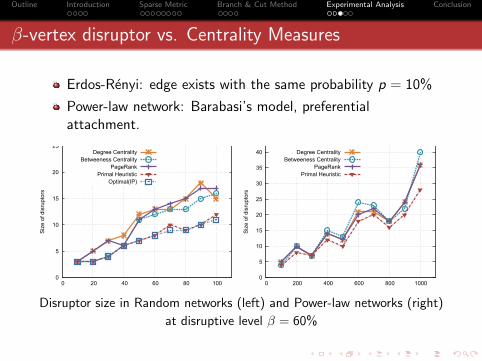
β-vertex disruptor vs. Centrality Measures

Compared methods:

1 Degree Centrality

2 Betweenness Centrality:Betweenness Bt(v) for vertex v is:

Bt(v) =∑

s 6=v 6=t∈Vs 6=t

σst(v)σst

where σst is the number of shortest

paths from s to t, and σst(v) is the number of shortest pathsfrom s to t that pass through a vertex v .

3 PageRank: Default damping factor of 85%

4 Primal heuristic: Primal heuristics in the B& C algorithm


β-vertex disruptor vs. Centrality Measures

Erdos-Renyi: edge exists with the same probability p = 10%

Power-law network: Barabasi’s model, preferentialattachment.

0

5

10

15

20

25

0 20 40 60 80 100

Siz

e of

dis

rupt

ors



Optimal(IP)

0

5

10

15

20

25

30

35

40

0 200 400 600 800 1000

Siz

e of

dis

rupt

ors



Disruptor size in Random networks (left) and Power-law networks (right)

at disruptive level β = 60%


Western Power Grid

10

100

1000

0 % 20 % 40 % 60 % 80 % 100 %

Siz

e of

dis

rupt

ors

Degree CentralityBetweeness CentralityEigenvector Centrality

Primal Heuristic

Vulnerability assessment of Western States Power Grid


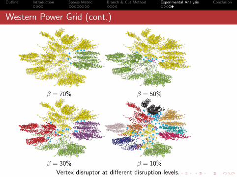
Western Power Grid (cont.)

β = 70% β = 50%

β = 30% β = 10%

Vertex disruptor at different disruption levels.


Summary

Propose Sparse metric technique to substantially removeunwanted constraints

A new Branch& Cut algorithm with a strong cutting plane

Results can be applied for β-edge disruptor, criticalnodes/edges detection and many connectivity-relatedproblems

Future work includes devising an efficient price-and-cutalgorithm based on the sparse metric.


Thank you for listening!Q&A

Precise Structural Vulnerability Assessment via Mathematical Programming

Documents

Transcript of Precise Structural Vulnerability Assessment via Mathematical Programming