Praktikum 4 - eau.eektanel/DK_0007/DK_prax4_eng.pdf · Praktikum 4 R and package Rcmdr : ... ☼ It...

Matemaatiline statistika ja modelleerimine, DK.0007

Tanel Kaart http://ph.emu.ee/~ktanel/DK_0007/ 1

Praktikum 4

R and package Rcmdr: frequency tables, χ2- and Fisher exact test;

correlation and regression analyses

1.

1.1. Open the R, and then load the R Workspace (.Rdata-fail) saved in last practical (Fail -> Load

Workspace …). If you haven’t what to load, follow the points 1.2 and 1.3 or 1.4.

1.2. Open the R Commander (for example running the command library(Rcmdr)).

If you had the R Workspace, then it contains also the students dataset and in R Commander you

should fix it as the default dataset for R Commander menus: .

1.3. If you haven’t the R Workspace what to load, you can import the csv-fail: students = read.csv("http://ph.emu.ee/~ktanel/DK_0007/studentsR_eng.csv", header=TRUE,

sep=";", dec=",")

and fix it.

1.4. As an alternative you may also import the Excel fail straight into the R Commander

(Data -> Import data -> from Excel, Access or dBase data set…).

2. Frequency tables, χ2- and Fisher exact test

2.1. The command Statistics -> Summaries -> Freguency distributions… in R Commander’s menus

allows to construct the frequency tables of nonnumeric traits and additionally to test using the χ2-

test, are the empirical frequencies counted from data different from some theoretical values.

For example you can test are both sexes distributed equally (50:50) or not:



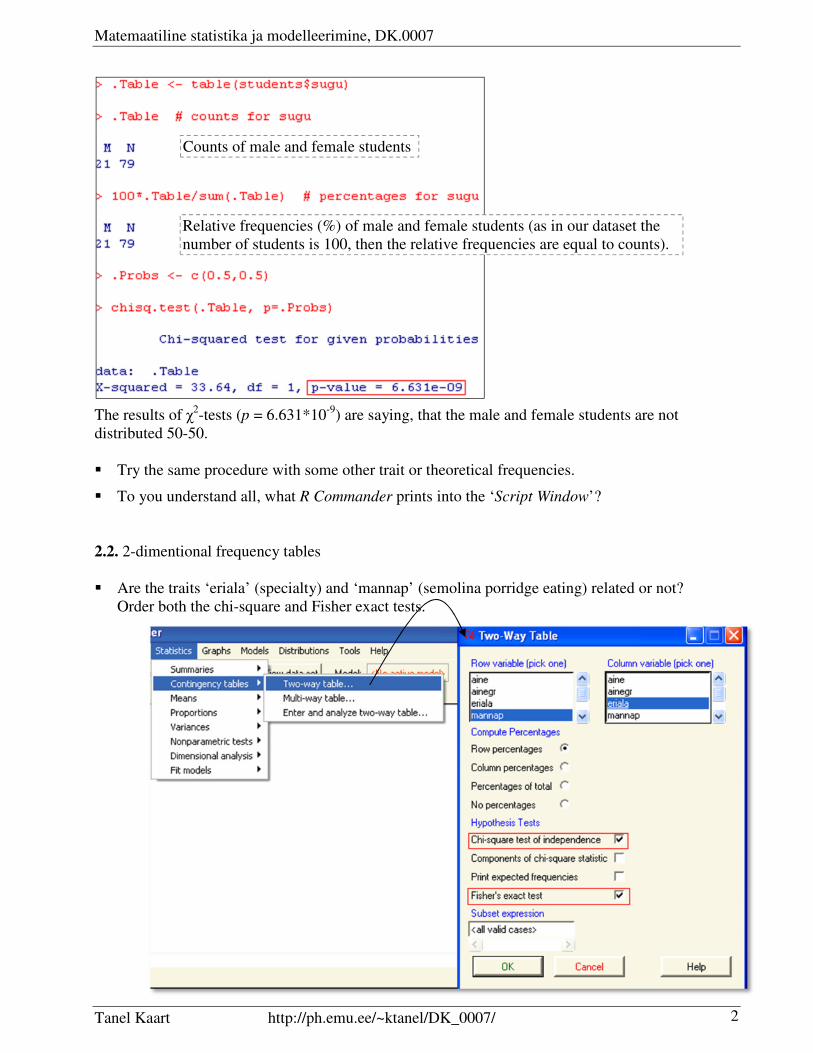
The results of χ2-tests (p = 6.631*10

-9) are saying, that the male and female students are not

distributed 50-50.

� Try the same procedure with some other trait or theoretical frequencies.

� To you understand all, what R Commander prints into the ‘Script Window’?

2.2. 2-dimentional frequency tables

� Are the traits ‘eriala’ (specialty) and ‘mannap’ (semolina porridge eating) related or not?

Order both the chi-square and Fisher exact tests.

Counts of male and female students

Relative frequencies (%) of male and female students (as in our dataset the

number of students is 100, then the relative frequencies are equal to counts).



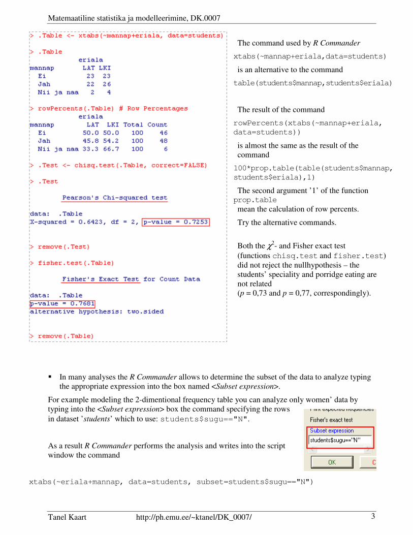
The command used by R Commander

xtabs(~mannap+eriala,data=students)

is an alternative to the command

table(students$mannap,students$eriala)

The result of the command

rowPercents(xtabs(~mannap+eriala,

data=students))

is almost the same as the result of the

command

100*prop.table(table(students$mannap,

students$eriala),1)

The second argument ’1’ of the function prop.table

mean the calculation of row percents.

Try the alternative commands.

Both the χ2- and Fisher exact test

(functions chisq.test and fisher.test)

did not reject the nullhypothesis – the

students’ speciality and porridge eating are

not related

(p = 0,73 and p = 0,77, correspondingly).

� In many analyses the R Commander allows to determine the subset of the data to analyze typing

the appropriate expression into the box named <Subset expression>.

For example modeling the 2-dimentional frequency table you can analyze only women’ data by

typing into the <Subset expression> box the command specifying the rows

in dataset ’students’ which to use: students$sugu=="N".

As a result R Commander performs the analysis and writes into the script

window the command

xtabs(~eriala+mannap, data=students, subset=students$sugu=="N")



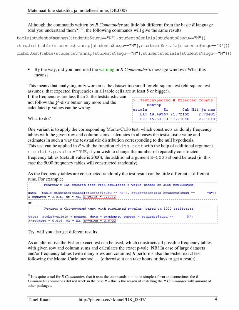
Although the commands written by R Commander are little bit different from the basic R language

(did you understand them?) ☼

, the following commands will give the same results:

table(students$mannap[students$sugu=="N"],students$eriala[students$sugu=="N"])

chisq.test(table(students$mannap[students$sugu=="N"],students$eriala[students$sugu=="N"]))

fisher.test(table(students$mannap[students$sugu=="N"],students$eriala[students$sugu=="N"]))

� By the way, did you mentined the warning in R Commander’s message window? What this

means?

This means that analysing only women is the dataset too small for chi-square test (chi-square test

assumes, that expected frequencies in all table cells are at least 5 or bigger).

If the frequencies are lass than 5, the teststatistic can

not follow the χ2-distribution any more and the

calculated p-values can be wrong.

What to do?

One variant is to apply the corresponding Monte-Carlo test, which constructs randomly frequency

tables with the given row and column sums, calculates in all cases the teststatistic value and

estimates in such a way the teststatistic distribution corresponding to the null hypothesis.

This test can be applied in R with the function chisq.test with the help of additional argument

simulate.p.value=TRUE, if you wish to change the number of repatedly constructed

frequency tables (default value is 2000), the additional argument B=5000 should be used (in this

case the 5000 frequency tables will constructed randomly).

As the frequency tables are constructed randomly the test result can be little different at different

runs. For example:

or

Try, will you also get diferent results.

As an alternative the Fisher excact test can be used, which constructs all possible frequency tables

with given row and column sums and calculates the exact p-vale. NB! In case of large datasets

and/or frequency tables (with many rows and columns) R performs also the Fisher exact test

following the Monte-Carlo method … (otherwise it can take hours or days to get a result).

☼

It is quite usual for R Commander, that it uses the commands not in the simplest form and sometimes the R

Commander commands did not work in the base R – this is the reason of installing the R Commander with amount of

other packages.



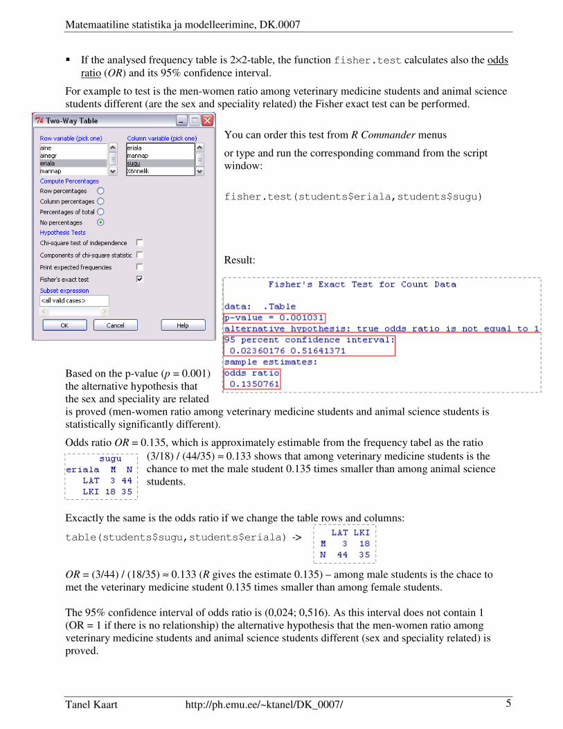
� If the analysed frequency table is 2×2-table, the function fisher.test calculates also the odds

ratio (OR) and its 95% confidence interval.

For example to test is the men-women ratio among veterinary medicine students and animal science

students different (are the sex and speciality related) the Fisher exact test can be performed.

You can order this test from R Commander menus

or type and run the corresponding command from the script

window:

fisher.test(students$eriala,students$sugu)

Result:

Based on the p-value (p = 0.001)

the alternative hypothesis that

the sex and speciality are related

is proved (men-women ratio among veterinary medicine students and animal science students is

statistically significantly different).

Odds ratio OR = 0.135, which is approximately estimable from the frequency tabel as the ratio

(3/18) / (44/35) ≈ 0.133 shows that among veterinary medicine students is the

chance to met the male student 0.135 times smaller than among animal science

students.

Excactly the same is the odds ratio if we change the table rows and columns:

table(students$sugu,students$eriala) ->

OR = (3/44) / (18/35) ≈ 0.133 (R gives the estimate 0.135) – among male students is the chace to

met the veterinary medicine student 0.135 times smaller than among female students.

The 95% confidence interval of odds ratio is (0,024; 0,516). As this interval does not contain 1

(OR = 1 if there is no relationship) the alternative hypothesis that the men-women ratio among

veterinary medicine students and animal science students different (sex and speciality related) is

proved.



3. Correlation analysis

3.1.

Find the correlations between numerical traits (except the year) using

a) whether the script window in R Commander:

cor(students[,c("bmi","kaal","mat","peaymb","pikkus")], use="pair")

Remarks:

¤) the missing first argument (before comma) in [,c("bmi","kaal","mat","peaymb","pikkus")]

says that all rows must be used, the second argument forms the list of used columns;

¤) simple command cor(students) finds correlations between all numerical variables

in dataset;

¤) cor(students$bmi, students$kaal) finds the correlation only between

mentioned variables;

¤) options use="pair" or use="complete.obs" are necessary, if dataset contains

missing values:

the second variant (use="complete.obs") asks R to omit all rows with missing

values for any of the study variable,

the first variant (use="pair") omits only rows with missing values for variables’

pair (for different correlations different number of observations can be used);

¤) by default the Pearson correlation coefficients are found,

for Spearman and Kendall correlation coefficients use the options

method="spearman" and method="kendall"

(also the Pearson correlation coefficient can be specified with method="pearson").

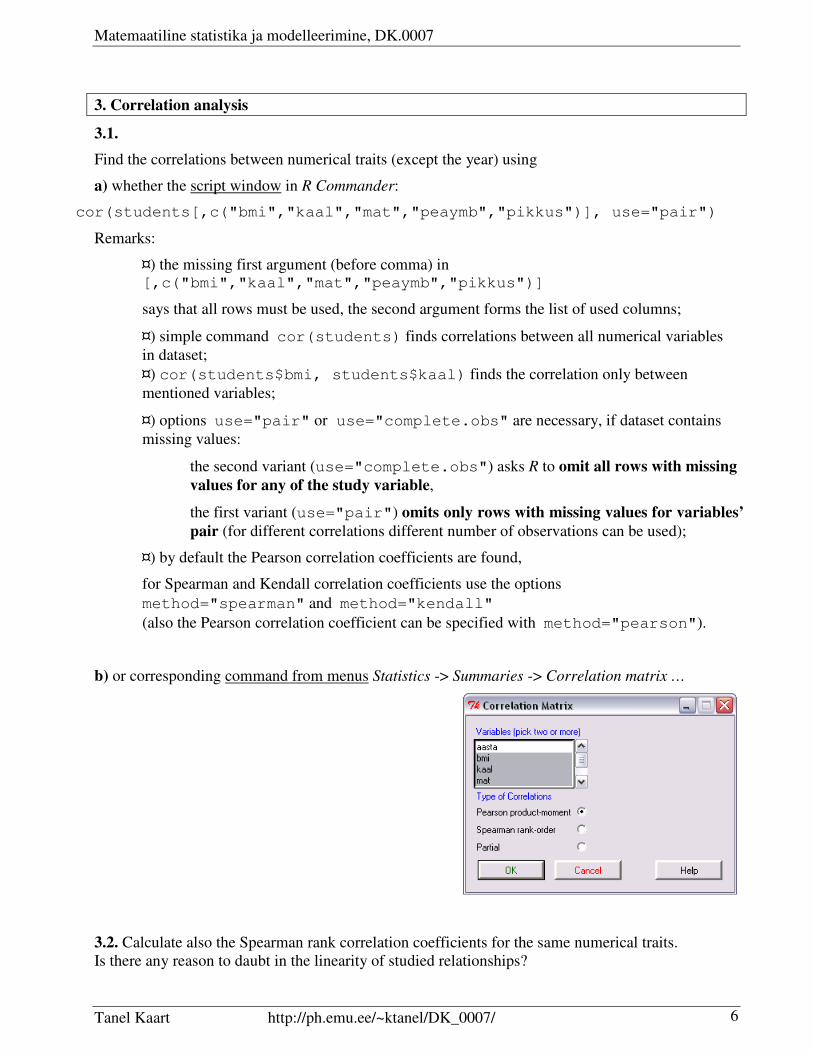
b) or corresponding command from menus Statistics -> Summaries -> Correlation matrix …

3.2. Calculate also the Spearman rank correlation coefficients for the same numerical traits.

Is there any reason to daubt in the linearity of studied relationships?



If there is no big difference between Spearman rank correlation and Pearson linear correlation

coefficients, then it is reasonable to use the last (it is more simple and more traditional).

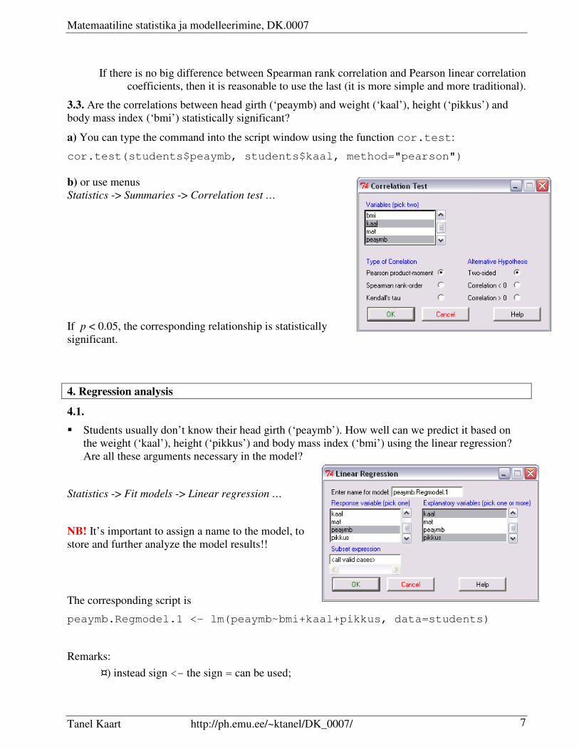
3.3. Are the correlations between head girth (‘peaymb) and weight (‘kaal’), height (‘pikkus’) and

body mass index (‘bmi’) statistically significant?

a) You can type the command into the script window using the function cor.test:

cor.test(students$peaymb, students$kaal, method="pearson")

b) or use menus

Statistics -> Summaries -> Correlation test …

If p < 0.05, the corresponding relationship is statistically

significant.

4. Regression analysis

4.1.

� Students usually don’t know their head girth (‘peaymb’). How well can we predict it based on

the weight (‘kaal’), height (‘pikkus’) and body mass index (‘bmi’) using the linear regression?

Are all these arguments necessary in the model?

Statistics -> Fit models -> Linear regression …

NB! It’s important to assign a name to the model, to

store and further analyze the model results!!

The corresponding script is

peaymb.Regmodel.1 <- lm(peaymb~bmi+kaal+pikkus, data=students)

Remarks:

¤) instead sign <- the sign = can be used;



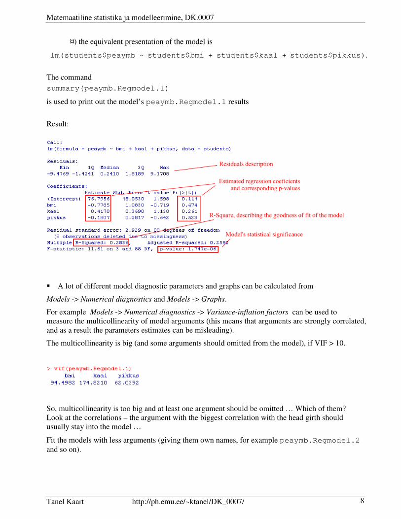
¤) the equivalent presentation of the model is

lm(students$peaymb ~ students$bmi + students$kaal + students$pikkus).

The command

summary(peaymb.Regmodel.1)

is used to print out the model’s peaymb.Regmodel.1 results

Result:

� A lot of different model diagnostic parameters and graphs can be calculated from

Models -> Numerical diagnostics and Models -> Graphs.

For example Models -> Numerical diagnostics -> Variance-inflation factors can be used to

measure the multicollinearity of model arguments (this means that arguments are strongly correlated,

and as a result the parameters estimates can be misleading).

The multicollinearity is big (and some arguments should omitted from the model), if VIF > 10.

So, multicollinearity is too big and at least one argument should be omitted … Which of them?

Look at the correlations – the argument with the biggest correlation with the head girth should

usually stay into the model …

Fit the models with less arguments (giving them own names, for example peaymb.Regmodel.2

and so on).



-2 -1 0 1 2

-10

-50

5

Normal Q-Q Plot

Theoretical Quantiles

Sam

ple

Qu

antile

s

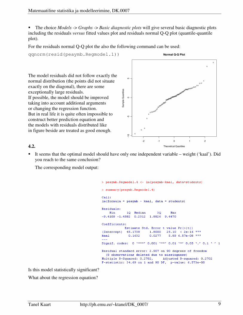
� The choice Models -> Graphs -> Basic diagnostic plots will give several basic diagnostic plots

including the residuals versus fitted values plot and residuals normal Q-Q plot (quantile-quantile

plot).

For the residuals normal Q-Q plot the also the following command can be used:

qqnorm(resid(peaymb.Regmodel.1))

The model residuals did not follow exactly the

normal distribution (the points did not situate

exactly on the diagonal), there are some

exceptionally large residuals.

If possible, the model should be improved

taking into account additional arguments

or changing the regression function.

But in real life it is quite often impossible to

construct better prediction equation and

the models with residuals distributed like

in figure beside are treated as good enough.

4.2.

� It seems that the optimal model should have only one independent variable – weight (‘kaal’). Did

you reach to the same conclusion?

The corresponding model output:

Is this model statistically significant?

What about the regression equation?



40 50 60 70 80 90 100-1

0-5

05

10

students$kaal

resid

(pe

aym

b.R

eg

mo

de

l.4

)

40 50 60 70 80 90 100

45

50

55

60

65

Students weight (kg)

Stu

de

nts

he

ad

gir

th (

cm

)

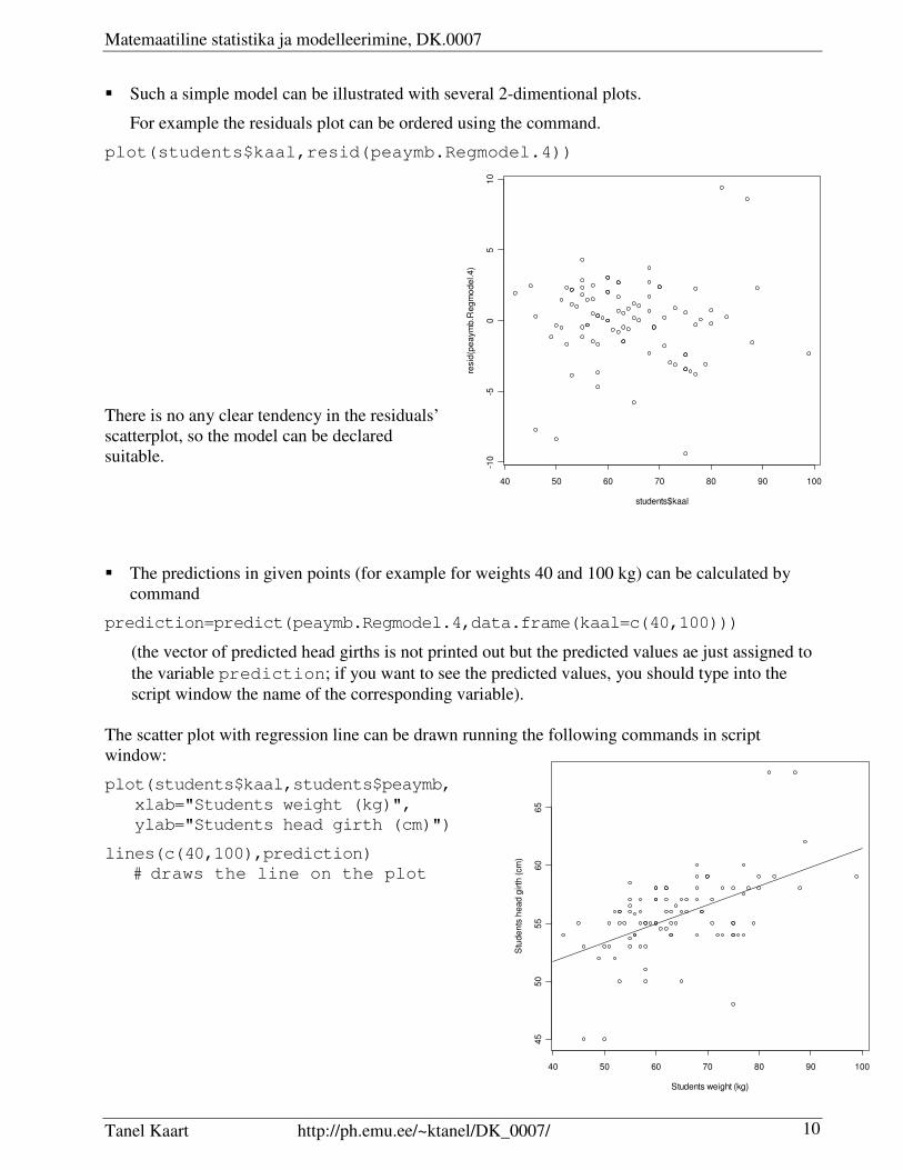
� Such a simple model can be illustrated with several 2-dimentional plots.

For example the residuals plot can be ordered using the command.

plot(students$kaal,resid(peaymb.Regmodel.4))

There is no any clear tendency in the residuals’

scatterplot, so the model can be declared

suitable.

� The predictions in given points (for example for weights 40 and 100 kg) can be calculated by

command

prediction=predict(peaymb.Regmodel.4,data.frame(kaal=c(40,100)))

(the vector of predicted head girths is not printed out but the predicted values ae just assigned to

the variable prediction; if you want to see the predicted values, you should type into the

script window the name of the corresponding variable).

The scatter plot with regression line can be drawn running the following commands in script

window:

plot(students$kaal,students$peaymb,

xlab="Students weight (kg)",

ylab="Students head girth (cm)")

lines(c(40,100),prediction)

# draws the line on the plot



40 50 60 70 80 90 1004

55

055

60

65


Stu

de

nts

he

ad

gir

th (

cm

)

On the same graph the tolerance and confidence intervals can be added using the commands

prediction=predict(peaymb.Regmodel.4,

data.frame(kaal=c(40:100)),interval="prediction")

lines(40:100,prediction[,2],lty=2)

lines(40:100,prediction [,3],lty=2)

prediction=predict(peaymb.Regmodel.4,

data.frame(kaal=c(40:100)),

interval="confidence")



(the 95% tolerance interval shows the area of 95%

students’ weights and head girths;

the 95% confidence interval is the area where the

real regression line should be with probability 0.95).

� The similar plot can be drawn also in R Commander:

Graphs -> Scatterplot …

The confidence and tolerance intervals are not

selectable in menus but these can be added

later using the commands predict and

lines in script window.

40 50 60 70 80 90 100

45

50

55

60

65


Stu

de

nts

he

ad

gir

th (

cm

)



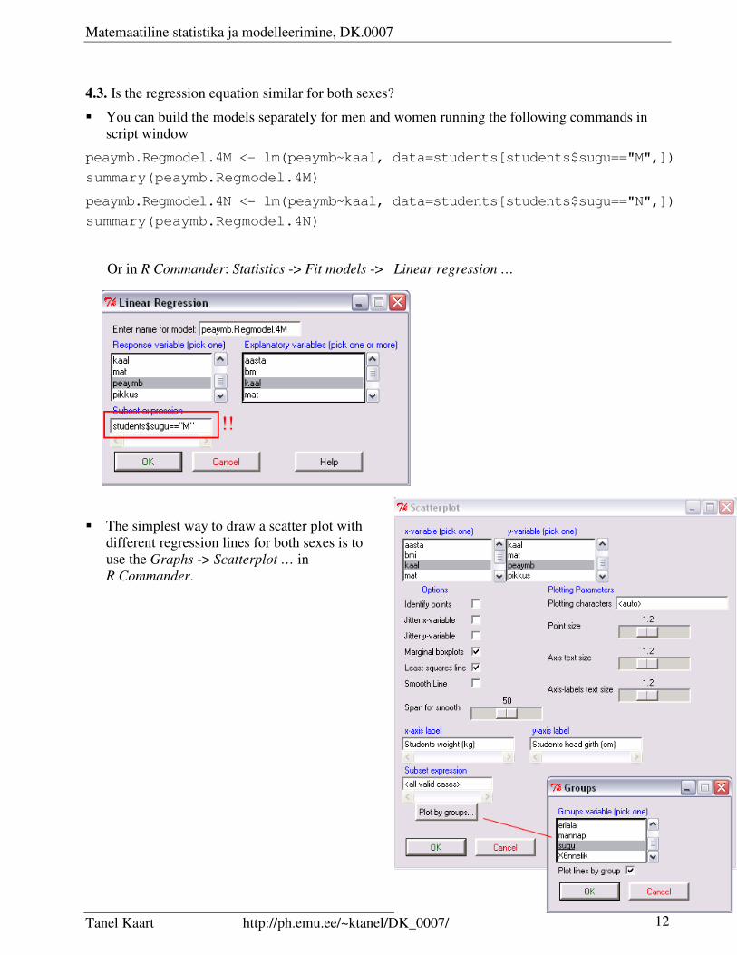
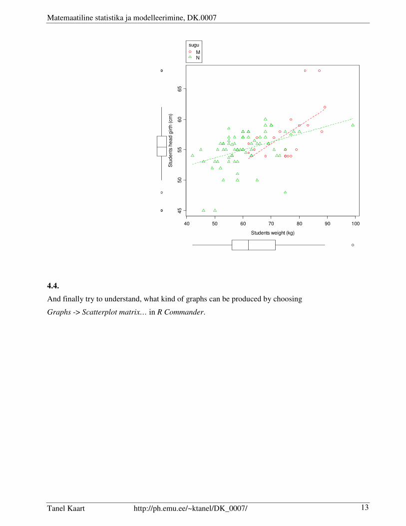
4.3. Is the regression equation similar for both sexes?

� You can build the models separately for men and women running the following commands in

script window

peaymb.Regmodel.4M <- lm(peaymb~kaal, data=students[students$sugu=="M",])

summary(peaymb.Regmodel.4M)

peaymb.Regmodel.4N <- lm(peaymb~kaal, data=students[students$sugu=="N",])

summary(peaymb.Regmodel.4N)

Or in R Commander: Statistics -> Fit models -> Linear regression …

� The simplest way to draw a scatter plot with

different regression lines for both sexes is to

use the Graphs -> Scatterplot … in

R Commander.



4.4.

And finally try to understand, what kind of graphs can be produced by choosing

Graphs -> Scatterplot matrix… in R Commander.

40 50 60 70 80 90 100

45

50

55

60

65


Stu

de

nts

he

ad

gir

th (

cm

)

sugu

MN

Praktikum 4 - eau.eektanel/DK_0007/DK_prax4_eng.pdf · Praktikum 4 R and package Rcmdr : ... ☼ It...

Documents

Transcript of Praktikum 4 - eau.eektanel/DK_0007/DK_prax4_eng.pdf · Praktikum 4 R and package Rcmdr : ... ☼ It...