PowerPoint 簡報 - 國立臺灣大學cc.ee.ntu.edu.tw/~wujsh/10101PC/Chapter3_101.11.05.pdfPulse...

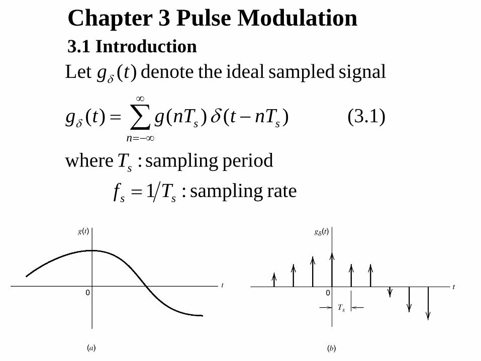
rate sampling:1 period sampling : where

(3.1) )( )()(

signal sampled ideal thedenote )(Let

ss

s

sn

s

TfT

nTtnTgtg

tg

=

−= ∑∞

−∞=

δδ

δ

Chapter 3 Pulse Modulation 3.1 Introduction

∑

∑

∑

∑

∑

∑

∑

∞

−∞=

∞

≠−∞=

∞

−∞=

∞

−∞=

∞

−∞=

∞

−∞=

∞

−∞=

−=

=≥=

−+=

−=

−⇔

−=

−∗

⇔−

n

s

mm

sss

sn

s

mss

mss

m ss

ns

W n fj

WngfG

WTWffG

mffGffGffG

nf TjnTgfG

mffGftg

mffGf

Tmf

TfG

nTtt

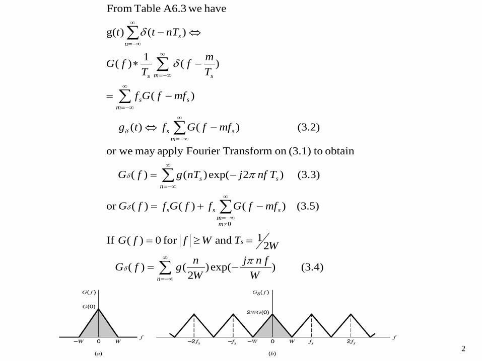
(3.4) )exp()2

()(

21 and for 0)( If

(3.5) )()()(or

(3.3) )2exp()()(

obtain to(3.1) on Transformier apply Fourmay or we

(3.2) )()(

)(

)(1)(

)()g(

have weA6.3 Table From

0

π

π

δ

δ

δ

δ

δ

δ

2

)( of ninformatio all contains )2

(or

for )2

(by determineduniquely is )(

(3.7) , )exp()2

(21)(

as )( rewritemay we(3.6) into (3.4) ngSubstituti

(3.6) , )(21)(

that (3.5) Equationfrom find we2.2

for 0)(.1 With

tgWng

nWngtg

WfWW

nfjWng

WfG

fG

WfWfGW

fG

WfWffG

n

s

∞<<∞−

<<−−=

<<−=

=

≥=

∑∞

−∞=

π

δ

3

)( offormula ioninterpolat an is (3.9)

(3.9) - , )2(sin)2

(

2

)2sin()2

(

(3.8) )2

(2exp 21)

2(

)2exp()exp()2

(21

)2exp()()(

havemay we, )2

( from )(t reconstruc To

tg

tnWtcWng

n Wtn Wt

Wng

dfWnt fj

WWng

df f tjW n fj

Wng

W

dfftjfGtg

Wngtg

n

n

n

W

W

W

Wn

∑

∑

∑ ∫

∫ ∑

∫

∞

−∞=

∞

−∞=

∞

−∞=−

−

∞

−∞=

∞

∞−

∞<<∞−=

−−

=

−=

−=

=

ππππ

π

ππ

π

4

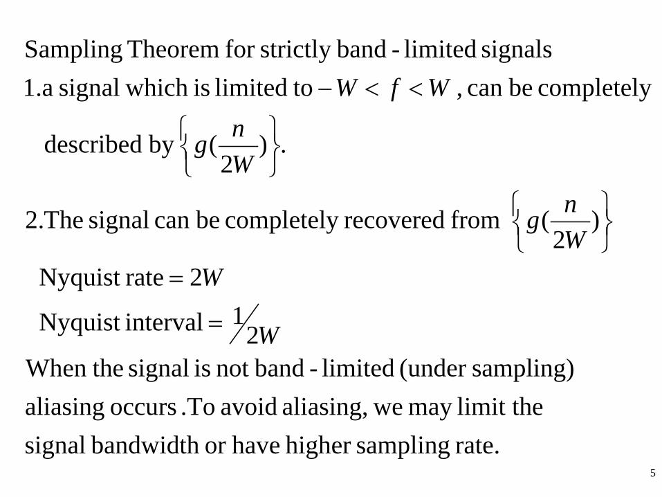
rate. samplinghigher haveor bandwidth signal limit themay wealiasing, avoid .To occurs aliasing

sampling)(under limited-bandnot is signal theWhen2

1 intervalNyquist

2 rateNyquist

)2

( from recovered completely be can signal The.2

.)2

(by described

completely be can , tolimited is whichsignal1.a signals limited-bandstrictly for Theorem Sampling

W

WWng

Wng

WfW

=

=

<<−

5

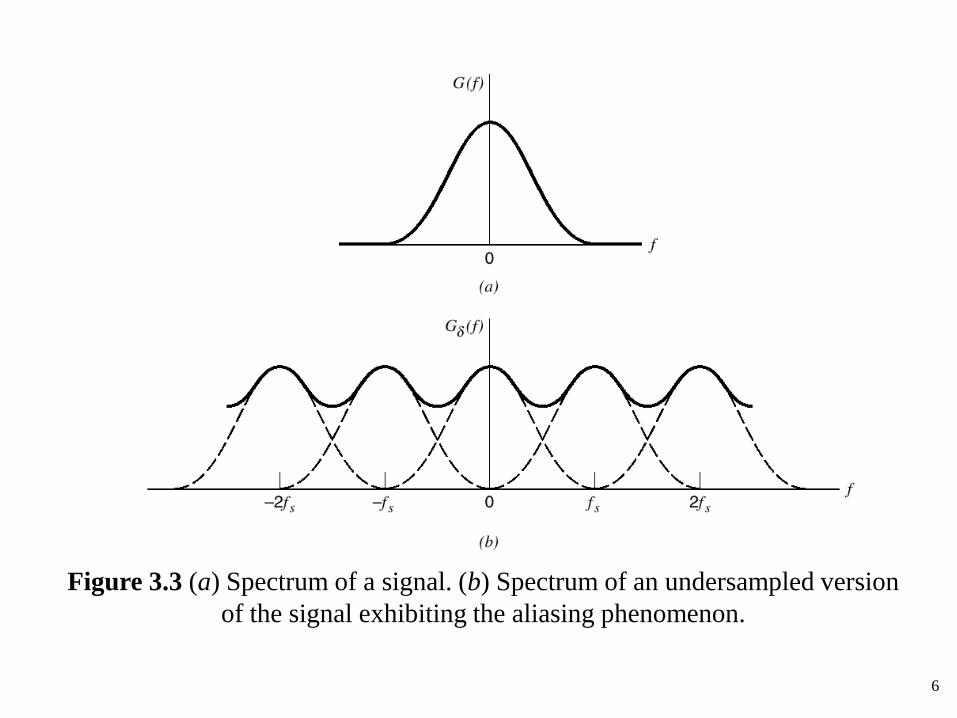
Figure 3.3 (a) Spectrum of a signal. (b) Spectrum of an undersampled version of the signal exhibiting the aliasing phenomenon.

6

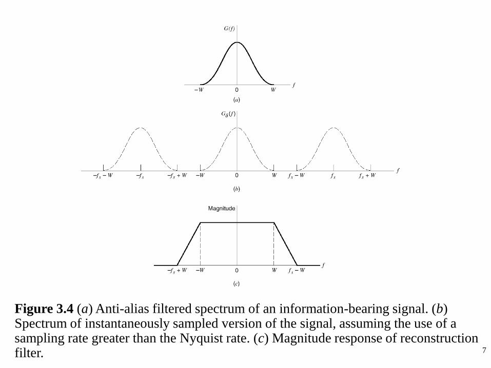
Figure 3.4 (a) Anti-alias filtered spectrum of an information-bearing signal. (b) Spectrum of instantaneously sampled version of the signal, assuming the use of a sampling rate greater than the Nyquist rate. (c) Magnitude response of reconstruction filter. 7

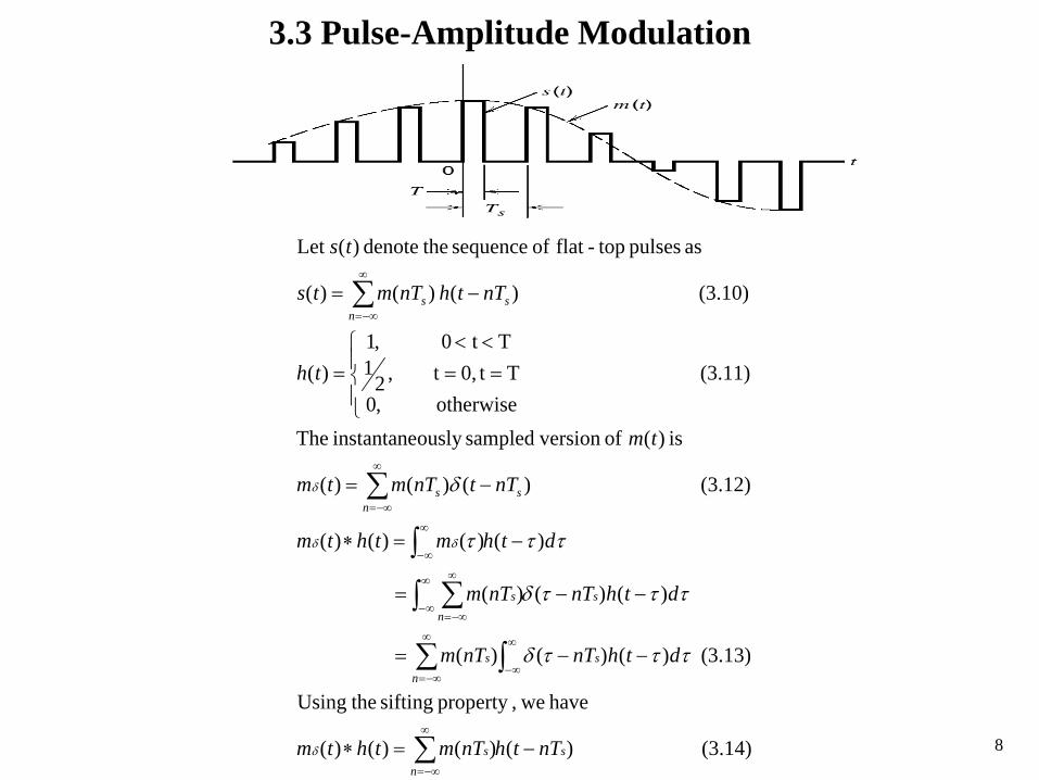
(3.14) )()()()(

have we,property sifting theUsing

(3.13) )()()(

)()()(

)()()()(

(3.12) )()()(

is )( of versionsampledously instantane The

(3.11) otherwise

Tt0,tTt 0

,,02

1,1

)(

(3.10) )( )()(

as pulses top-flat of sequence thedenote )(Let

sn

s

sn

s

sn

s

nss

sn

s

nTthnTmthtm

dthnTnTm

dthnTnTm

dthmthtm

nTtnTmtm

tm

th

nTthnTmts

ts

−=∗

−−=

−−=

−=∗

−=

==<<

=

−=

∑

∫∑

∫ ∑

∫

∑

∑

∞

−∞=

∞

∞−

∞

−∞=

∞

∞−

∞

−∞=

∞

∞−

∞

−∞=

∞

−∞=

δ

δδ

δ

τττδ

τττδ

τττ

δ

3.3 Pulse-Amplitude Modulation

8

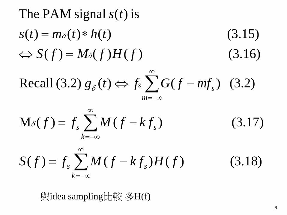
(3.18) )()()(

(3.17) )()(M

(3.2) )()( (3.2) Recall

(3.16) )()()((3.15) )()()(

is )( signal PAM The

∑

∑

∑

∞

−∞=

∞

−∞=

∞

−∞=

−=

−=

−⇔

=⇔∗=

kss

kss

mss

δ

fHk ffMffS

k ffMff

mffGftg

fHfMfSthtmts

ts

δ

δ

δ

9

與idea sampling比較多H(f)

Pulse Amplitude Modulation – Natural and Flat-Top Sampling

The circuit of Figure 11-3 is used to illustrate pulse amplitude modulation (PAM). The FET is the switch used as a sampling gate.

When the FET is on, the analog voltage is shorted to ground; when off, the FET is essentially open, so that the analog signal sample appears at the output.

Op-amp 1 is a noninverting amplifier that isolates the analog input channel from the switching function.

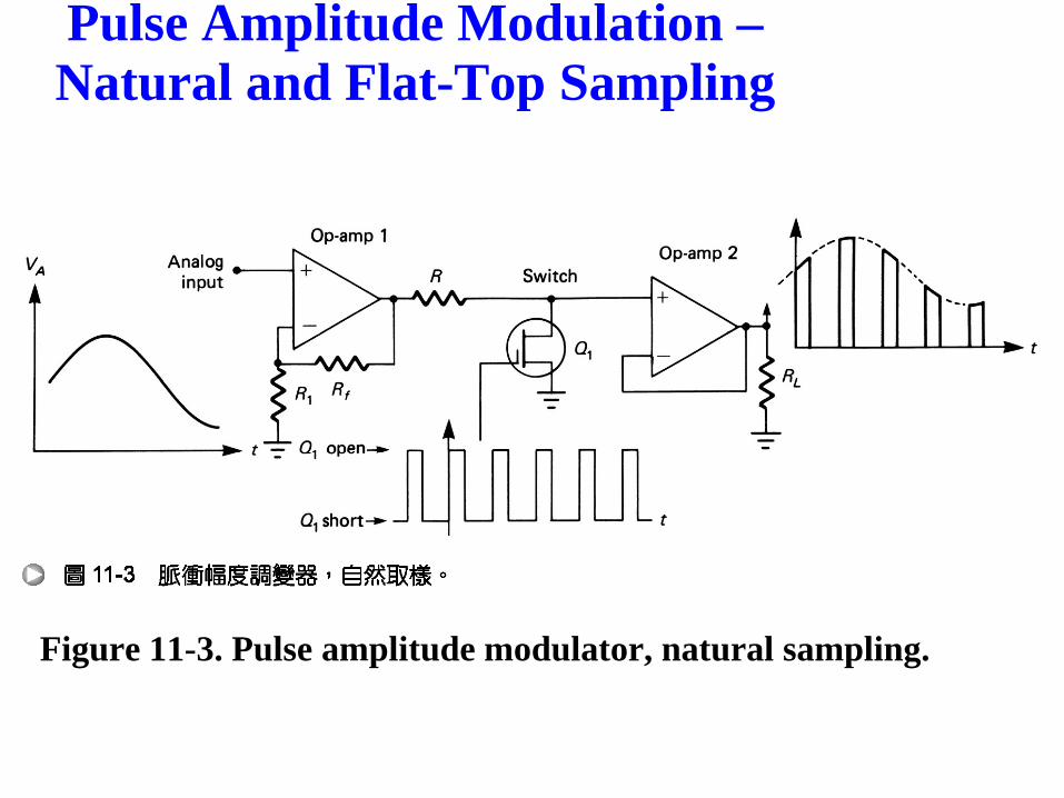
Figure 11-3. Pulse amplitude modulator, natural sampling.


Op-amp 2 is a high input-impedance voltage follower capable of driving low-impedance loads (high “fanout”).

The resistor R is used to limit the output current of op-amp 1 when the FET is “on” and provides a voltage division with rd of the FET. (rd, the drain-to-source resistance, is low but not zero)


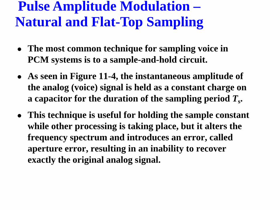
The most common technique for sampling voice in PCM systems is to a sample-and-hold circuit.

As seen in Figure 11-4, the instantaneous amplitude of the analog (voice) signal is held as a constant charge on a capacitor for the duration of the sampling period Ts.

This technique is useful for holding the sample constant while other processing is taking place, but it alters the frequency spectrum and introduces an error, called aperture error, resulting in an inability to recover exactly the original analog signal.


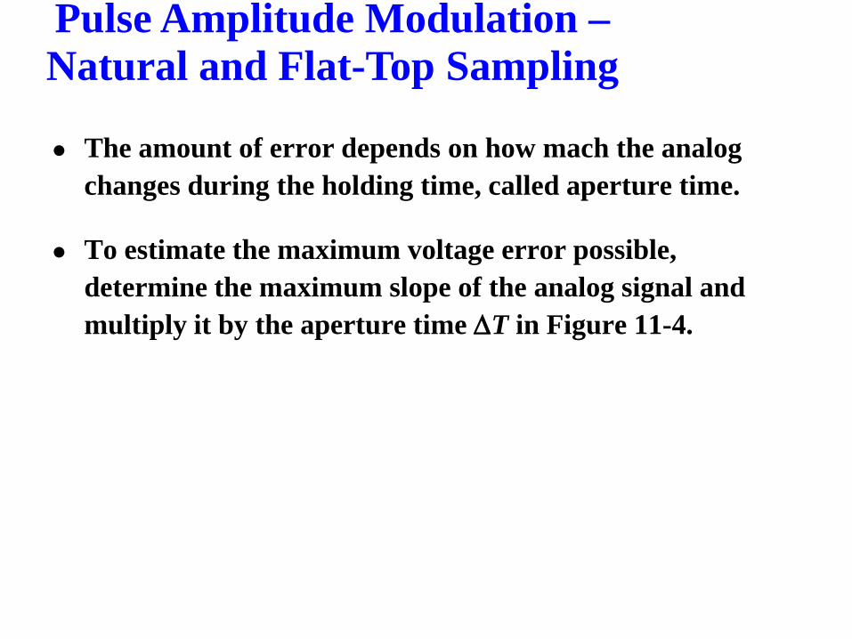
The amount of error depends on how mach the analog changes during the holding time, called aperture time.

To estimate the maximum voltage error possible, determine the maximum slope of the analog signal and multiply it by the aperture time ∆T in Figure 11-4.


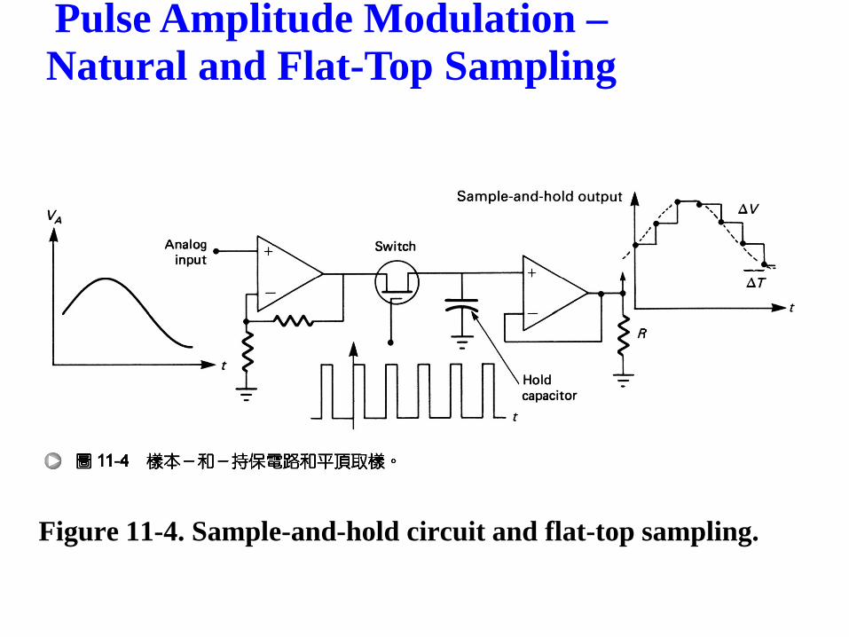
Figure 11-4. Sample-and-hold circuit and flat-top sampling.



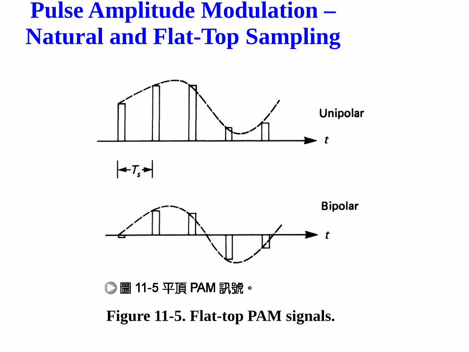
Figure 11-5. Flat-top PAM signals.

Wf M f H f k o in

h tH f T f T j f Tπ

=

= −

s

amplitude distort

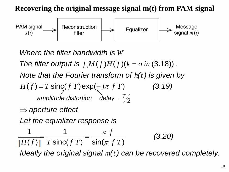
Where the filter bandwidth is The filter output is . Note that the Fourier transform of ( ) is given by

(3.19)

( ) ( )( (3.18))

( ) sinc( )exp( )T

fH f T f T f T

m t

ππ

=

⇒

= =

ion delay aperture effect

Let the equalizer response is

(3.20)

Ideally the original signal ( ) can be recovered completely.

2

1 1( ) sinc( ) sin( )

Recovering the original message signal m(t) from PAM signal

10

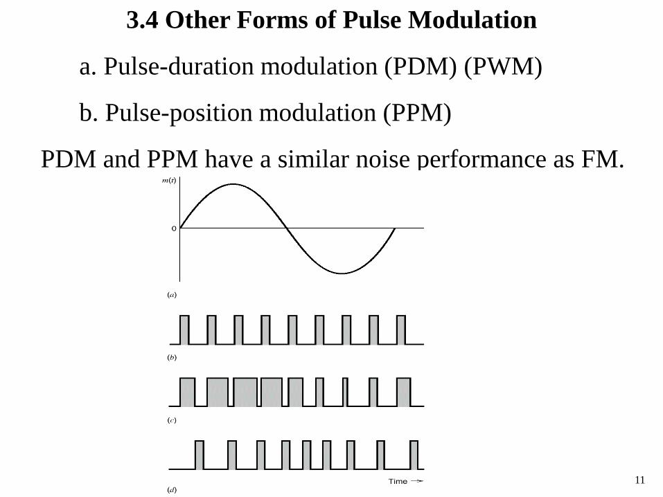
3.4 Other Forms of Pulse Modulation

a. Pulse-duration modulation (PDM) (PWM)

b. Pulse-position modulation (PPM)

PDM and PPM have a similar noise performance as FM.

11

In pulse width modulation (PWM), the width of each pulse is made directly proportional to the amplitude of the information signal.

In pulse position modulation, constant-width pulses are used, and the position or time of occurrence of each pulse from some reference time is made directly proportional to the amplitude of the information signal.

PWM and PPM are compared and contrasted to PAM in Figure 11-11.

Pulse Width and Pulse Position Modulation

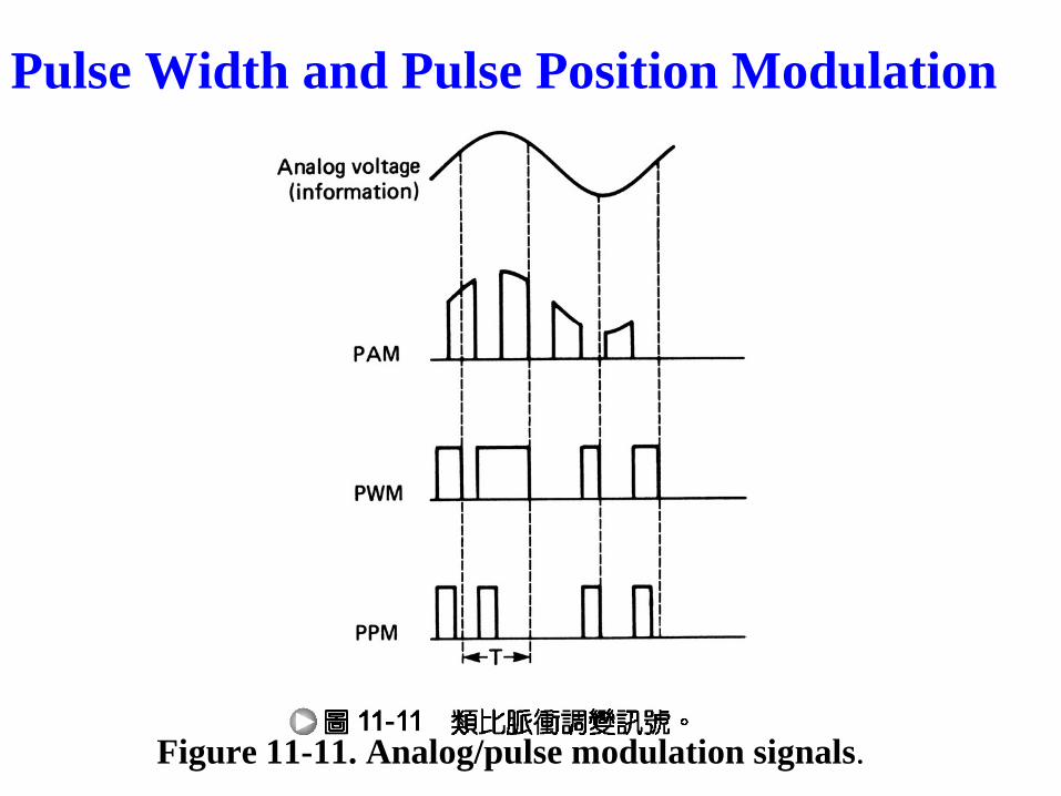
Figure 11-11. Analog/pulse modulation signals.


Figure 11-12 shows a PWM modulator. This circuit is simply a high-gain comparator that is switched on and off by the sawtooth waveform derived from a very stable-frequency oscillator.

Notice that the output will go to +Vcc the instant the analog signal exceeds the sawtooth voltage.

The output will go to -Vcc the instant the analog signal is less than the sawtooth voltage. With this circuit the average value of both inputs should be nearly the same.

This is easily achieved with equal value resistors to ground. Also the +V and –V values should not exceed Vcc.


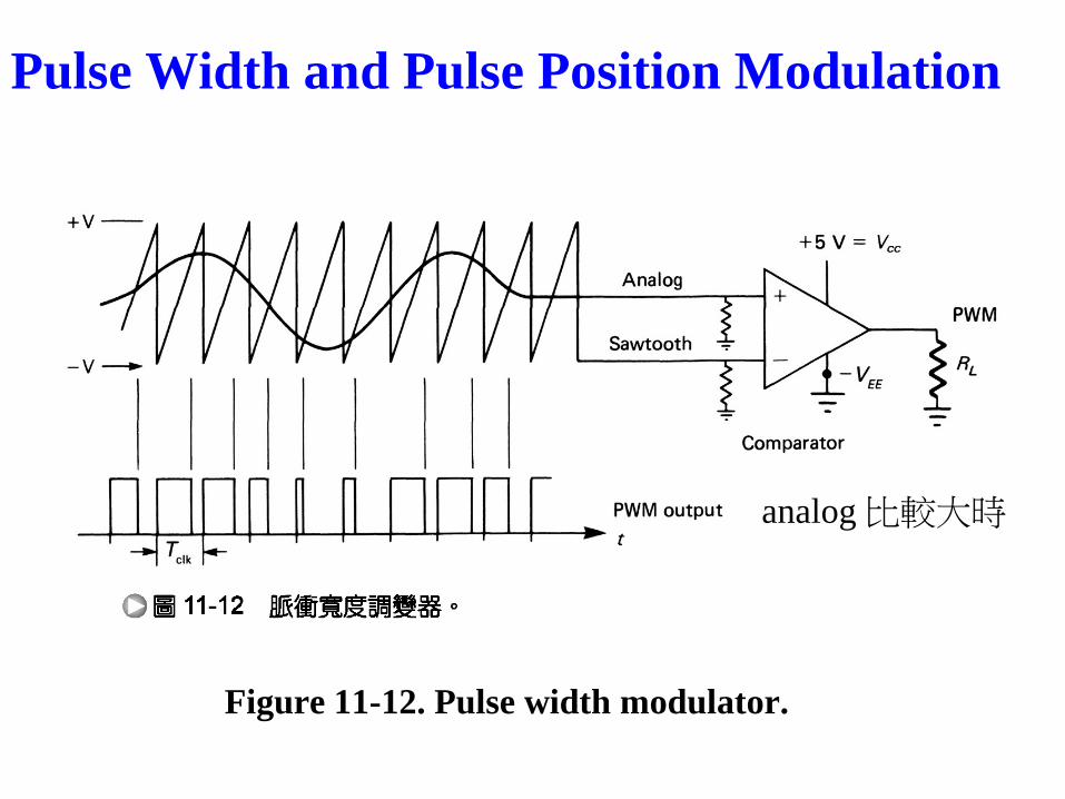
Figure 11-12. Pulse width modulator.


analog 比較大時

A 710-type IC comparator can be used for positive-only output pulses that are also TTL compatible. PWM can also be produced by modulation of various voltage-controllable multivibrators.

One example is the popular 555 timer IC. Other (pulse output) VCOs, like the 566 and that of the 565 phase-locked loop IC, will produce PWM.

This points out the similarity of PWM to continuous analog FM. Indeed, PWM has the advantages of FM---constant amplitude and good noise immunity---and also its disadvantage---large bandwidth.


Since the width of each pulse in the PWM signal shown in Figure 11-13 is directly proportional to the amplitude of the modulating voltage.

The signal can be differentiated as shown in Figure 11-13 (to PPM in part a), then the positive pulses are used to start a ramp, and the negative clock pulses stop and reset the ramp.

This produces frequency-to-amplitude conversion (or equivalently, pulse width-to-amplitude conversion).

The variable-amplitude ramp pulses are then time-averaged (integrated) to recover the analog signal.

Demodulation

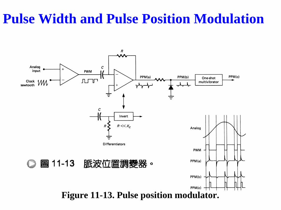
Figure 11-13. Pulse position modulator.


Demodulation

As illustrated in Figure 11-14, a narrow clock pulse sets an RS flip-flop output high, and the next PPM pulses resets the output to zero.

The resulting signal, PWM, has an average voltage proportional to the time difference between the PPM pulses and the reference clock pulses.

Time-averaging (integration) of the output produces the analog variations.

PPM has the same disadvantage as continuous analog phase modulation: a coherent clock reference signal is necessary for demodulation.

The reference pulses can be transmitted along with the PPM signal.

This is achieved by full-wave rectifying the PPM pulses of Figure 11-13a, which has the effect of reversing the polarity of the negative (clock-rate) pulses.

Then an edge-triggered flipflop (J-K or D-type) can be used to accomplish the same function as the RS flip-flop of Figure 11-14, using the clock input.

The penalty is: more pulses/second will require greater bandwidth, and the pulse width limit the pulse deviations for a given pulse period.

Demodulation

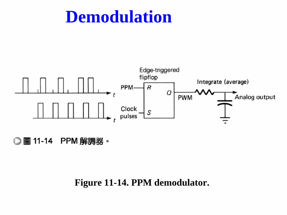
Figure 11-14. PPM demodulator.

Demodulation

Pulse Code Modulation (PCM)

Pulse code modulation (PCM) is produced by analog-to-digital conversion process.

As in the case of other pulse modulation techniques, the rate at which samples are taken and encoded must conform to the Nyquist sampling rate.

The sampling rate must be greater than, twice the highest frequency in the analog signal,

fs > 2fA(max)

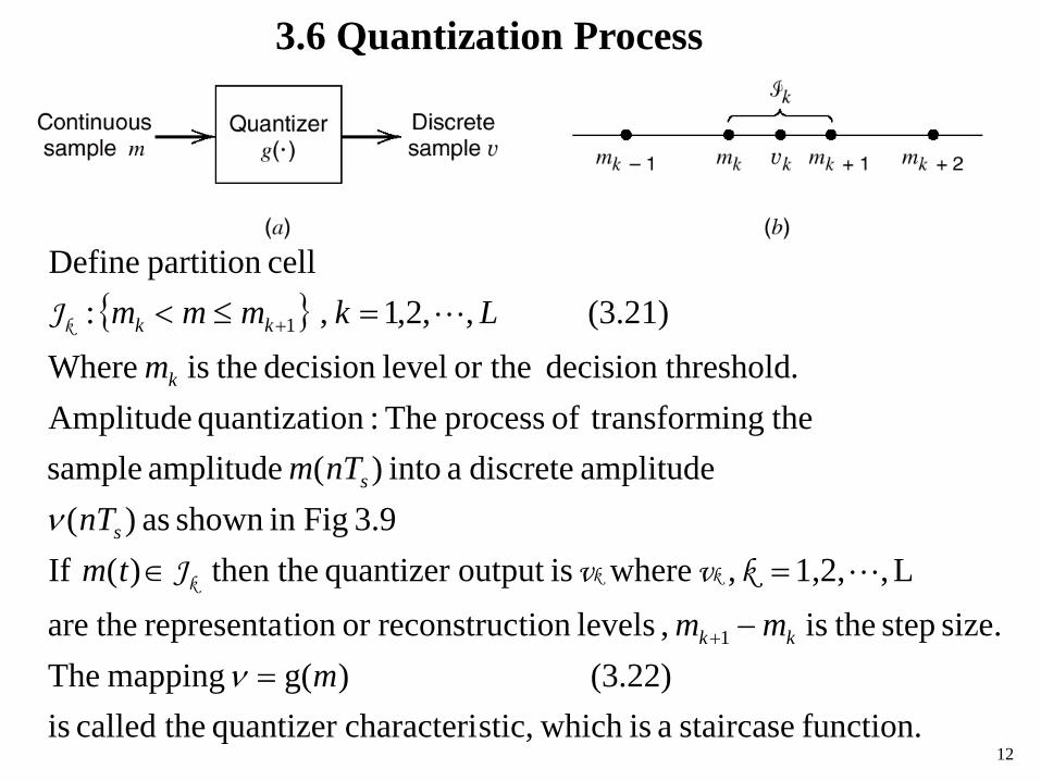
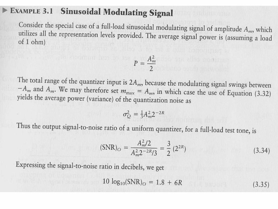
3.6 Quantization Process

{ }

function. staircasea is whichstic,characteriquantizer thecalled is(3.22) )g( mapping The

size. step theis , levels tionreconstrucor tionrepresenta theare L,1,2, , where isoutput quantizer the then )( If

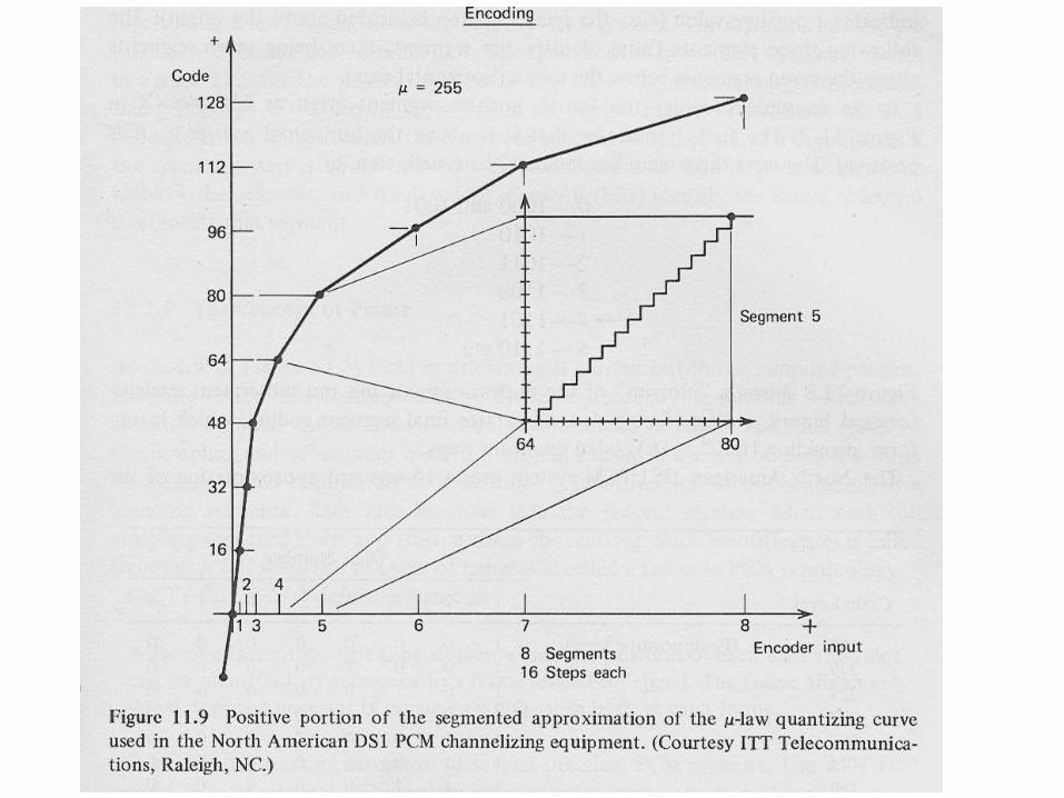
3.9 Figin shown as )(amplitude discretea into )( amplitude sample

theing transformof process The:onquantizati Amplitude. thresholddecision or the level decision theis Where

(3.21) ,,2,1 , :cell partition Define

1

1

mmm

tmnT

nTm

mLkmmm

kk

s

s

k

kk

=−

=∈

=≤<

+

+

ν

ν

kννJ

J

kkk

k

12

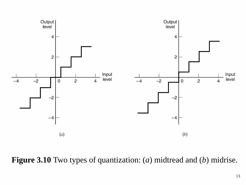
Figure 3.10 Two types of quantization: (a) midtread and (b) midrise.

13

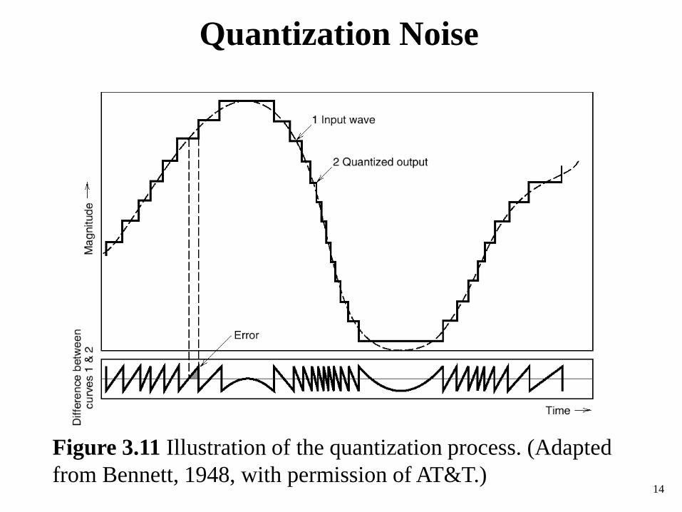
Quantization Noise

Figure 3.11 Illustration of the quantization process. (Adapted from Bennett, 1948, with permission of AT&T.)

14

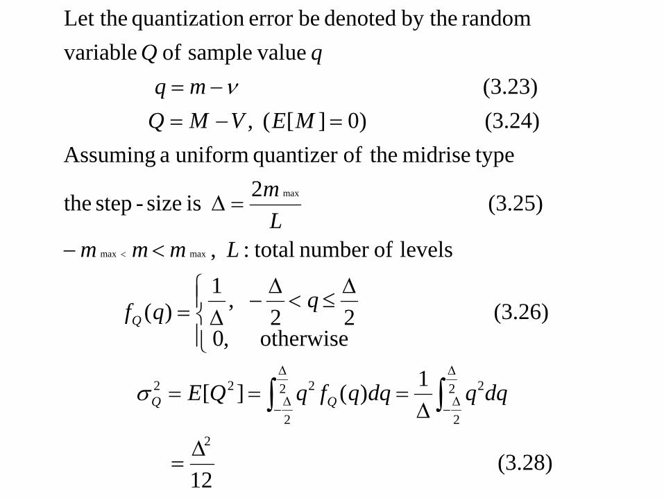
(3.28) 12

1)(][

(3.26) otherwise

2

2 ,0

,1)(

levels ofnumber total: ,

(3.25) 2 is size-step the

typemidrise theofquantizer uniforma Assuming(3.24) )0][( , (3.23)

valuesample of variable random by the denoted beerror onquantizati Let the

2

2

2

22

2

222

max max

max

∆=

∆===

∆

≤<∆

−∆=

<−

=∆

=−=−=

∫∫∆

∆−

∆

∆−

<

dqqdqqfqQE

qqf

LmmmL

m

MEVMQmq

qQ

QQ

Q

σ

ν

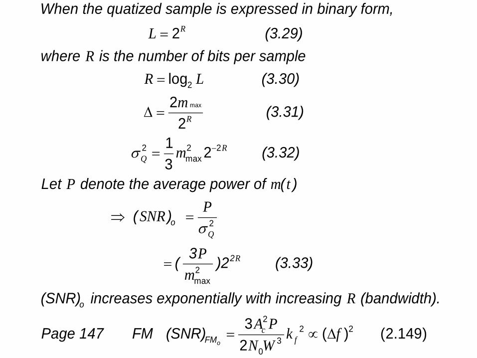
When the quatized sample is expressed in binary form, (3.29)where is the number of bits per sample (3.302

2

log

RLR

R L

=

=

o

)

(3.31)

(3.32)

Let denote the average power of ( )

( )

max

2 2 2max

2

22

1 23

R

RQ

Q

m

m

P m tPSNR

σ

σ

−

∆ =

=

⇒ =

o

2

o

FM

3 ( )2 (3.33)

(SNR) increases exponentially with increasing (bandwidth).

Page 147 FM (SNR)

2max

22 2

30

3 ( ) (2.149)2

R

cf

Pm

R

A P k fN W

=

= ∝ ∆

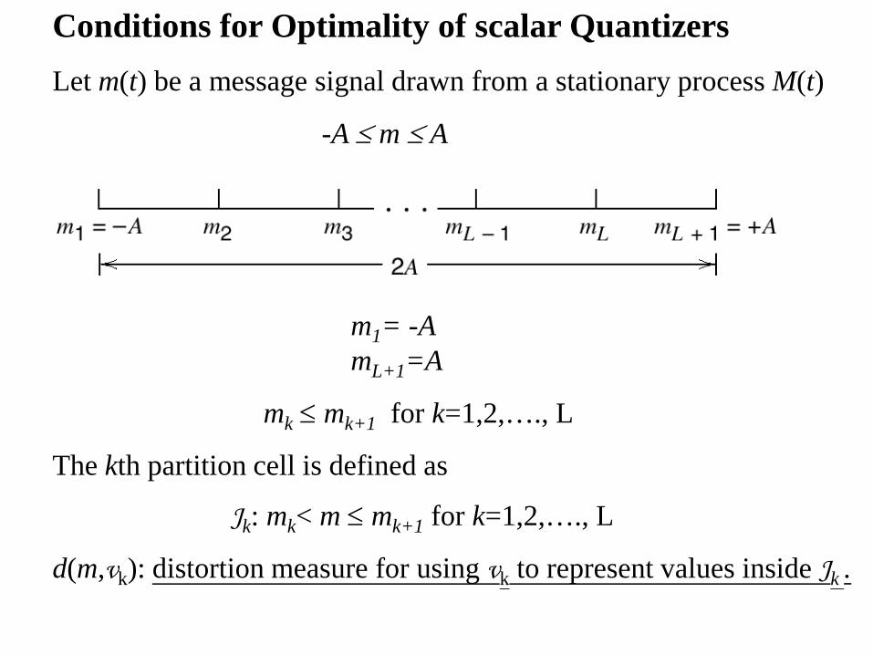
Conditions for Optimality of scalar Quantizers Let m(t) be a message signal drawn from a stationary process M(t)

-A ≤ m ≤ A

m1= -A mL+1=A

mk ≤ mk+1 for k=1,2,…., L

The kth partition cell is defined as

Jk: mk< m ≤ mk+1 for k=1,2,…., L

d(m,vk): distortion measure for using vk to represent values inside Jk .

{ } { }

kk

kk

M

M

L

km k

Lkk

Lkk

mmd

mf

dmmfmdDk

ν

νν

ν

ν

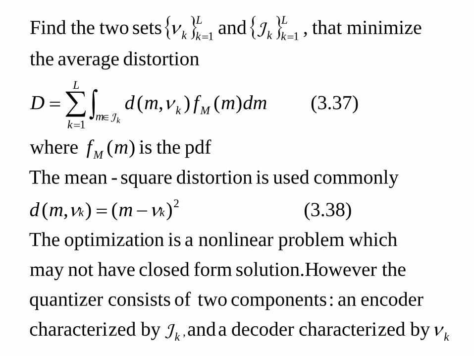
by zedcharacteridecoder a andby zedcharacteriencoder an: components twoof consistsquantizer

owever thesolution.H form closed havenot may whichproblemnonlinear a is onoptimizati The

(3.38) )( ),(commonly used is distortion square-mean The

pdf theis )( where

(3.37) )(),(

distortion average the minimize that , and sets two theFind

,

2

1

11

J

J

J

−=

= ∑∫=

∈

==

{ } { }

[ ]

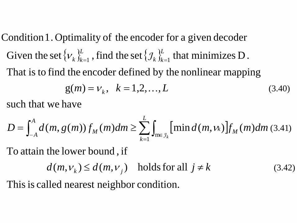
condition.neighbor nearest called is This allfor holds ),(),(

if , boundlower theattain To

)(),(min)())(,(

have that wesuch ,,1,2 ,)g(

mappingnonlinear by the definedencoder thefind toisThat . Dminimizes that set thefind , set theGiven

decoder givena for encoder theof Optimality . 1 Condition

(3.42)

)41.3(

(3.40)

1m

11

kjmdmd

dmmfmddmmfmgmdD

Lkm

jk

M

L

kk

A

A M

k

Lkk

Lkk

k

≠≤

≥=

==

∑∫∫=

∈−

==

νν

ν

ν

ν

J

J

{ } { }

k

L Lk kk k

L

k Mm

D

D m f m dm

ν

ν

= =

∈=

= −∑∫k 1

(3.43)

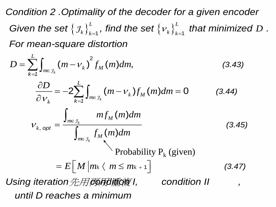
Condition 2 .Optimality of the decoder for a given encoder

Given the set , find the set that minimized .

For mean-square distortion

1 1

2( ) ( ) ,

J

J

k

k

k

L

k Mmk

Mmk

Mm

k k

D m f m dm

m f m dm

f m dm

E M m m m

νν

ν

∈=

∈

∈

+

∂= − − =

∂

=

= ⟨ ≤

∑∫

∫∫

k 1

opt

(3.44)

(3.45)

(3.47)

Usi

,

1

2 ( ) ( ) 0

( )

( )

J

J

J

ng iteration condition I, condition II , until D reaches a minimum

先用再用重複

Probability Pk (given)

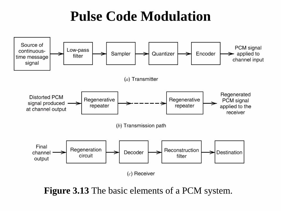
Figure 3.13 The basic elements of a PCM system.

Pulse Code Modulation

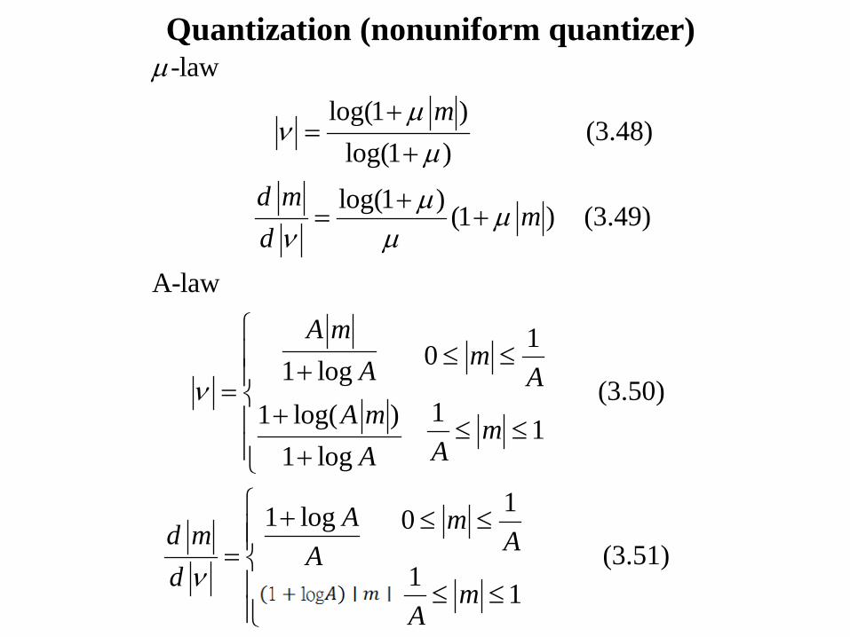
Quantization (nonuniform quantizer) -law

log(1 ) (3.48)

log(1 )

log(1 ) (1 ) (3.49)

A-law

101 log (3.50)

11 log( ) 11 log

1 log 0

(1 )

m

d mm

d

A mmA A

A m mAA

Ad mA

d A m

µµ

νµ

µ µν µ

ν

ν

+=

+

+= +

≤ ≤ +=

+ ≤ ≤ +

+=

+

1

(3.51)1 1

mA

mA

≤ ≤ ≤ ≤

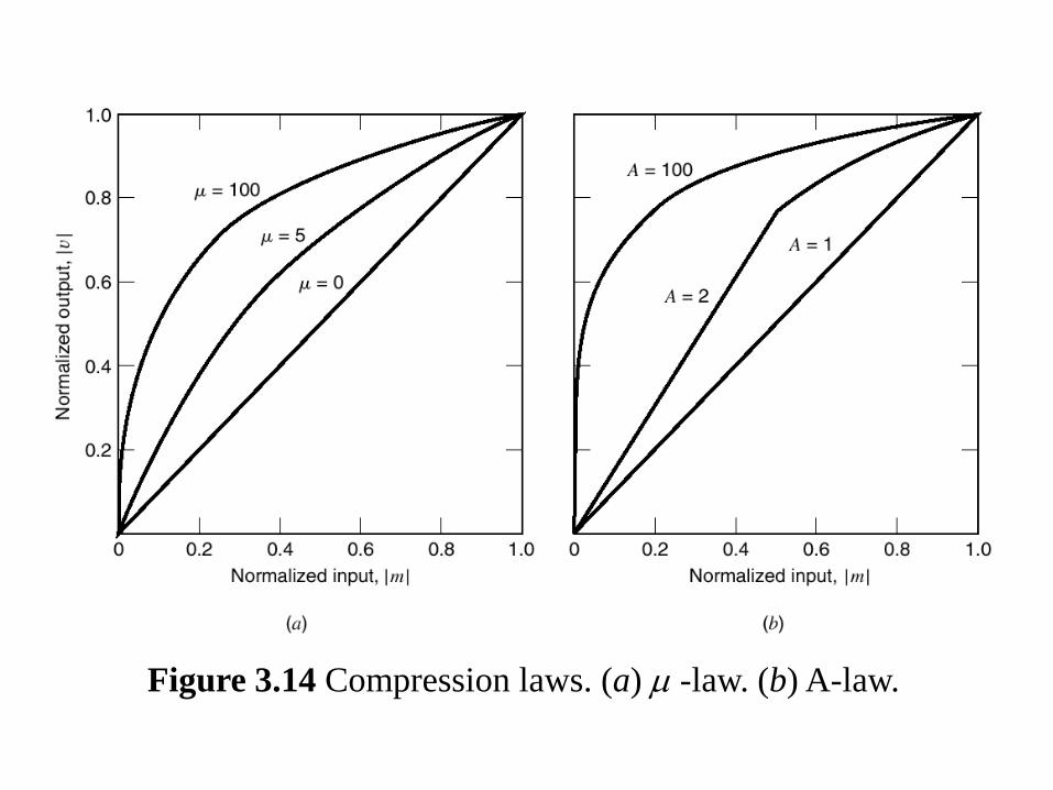
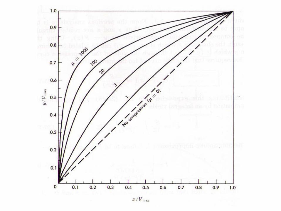
Figure 3.14 Compression laws. (a) µ -law. (b) A-law.

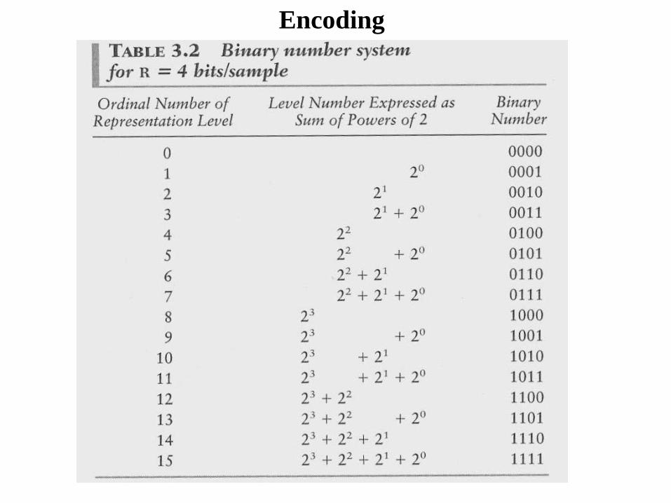
Encoding

1. Unipolar nonreturn-to-zero (NRZ) Signaling

2. Polar nonreturn-to-zero(NRZ) Signaling

3. Unipolar return-to-zero (RZ) Signaling

4. Bipolar return-to-zero (BRZ) Signaling

5. Split-phase (Manchester code)

Line codes:

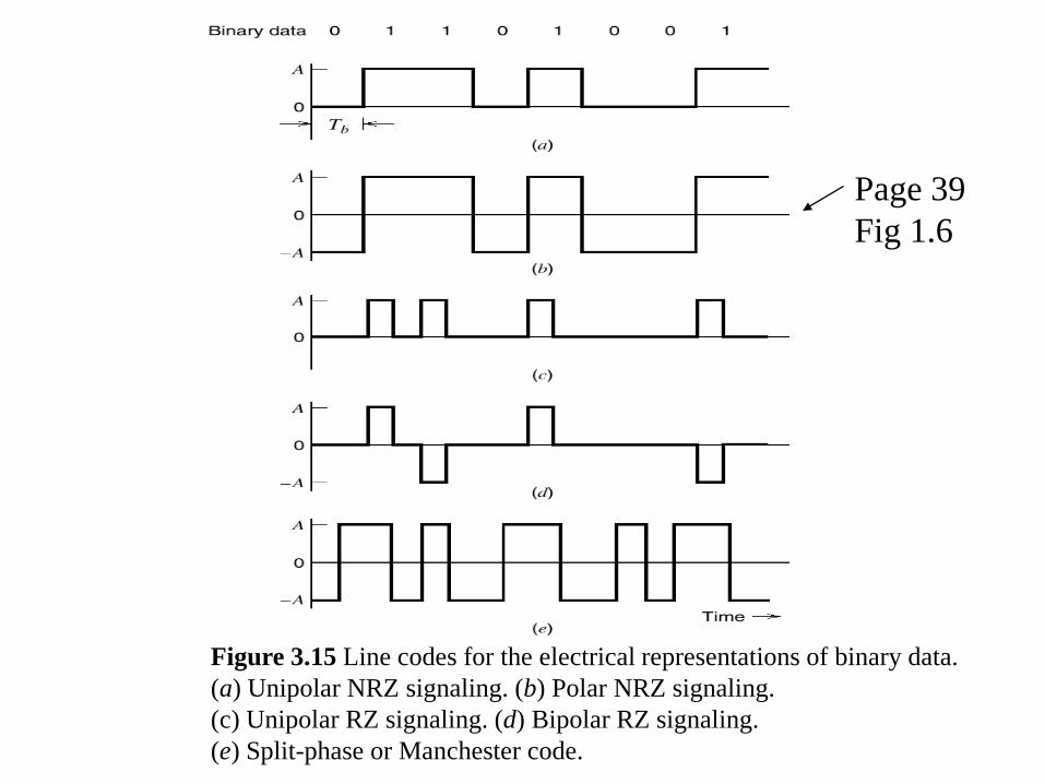
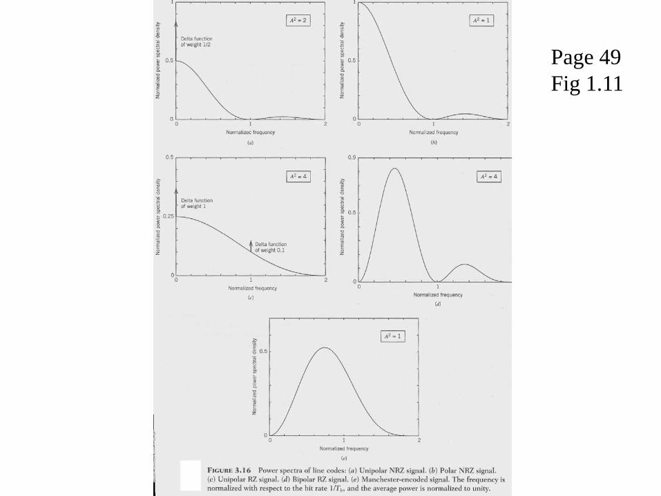
Figure 3.15 Line codes for the electrical representations of binary data. (a) Unipolar NRZ signaling. (b) Polar NRZ signaling. (c) Unipolar RZ signaling. (d) Bipolar RZ signaling. (e) Split-phase or Manchester code.

Page 39 Fig 1.6

Fig 1.11

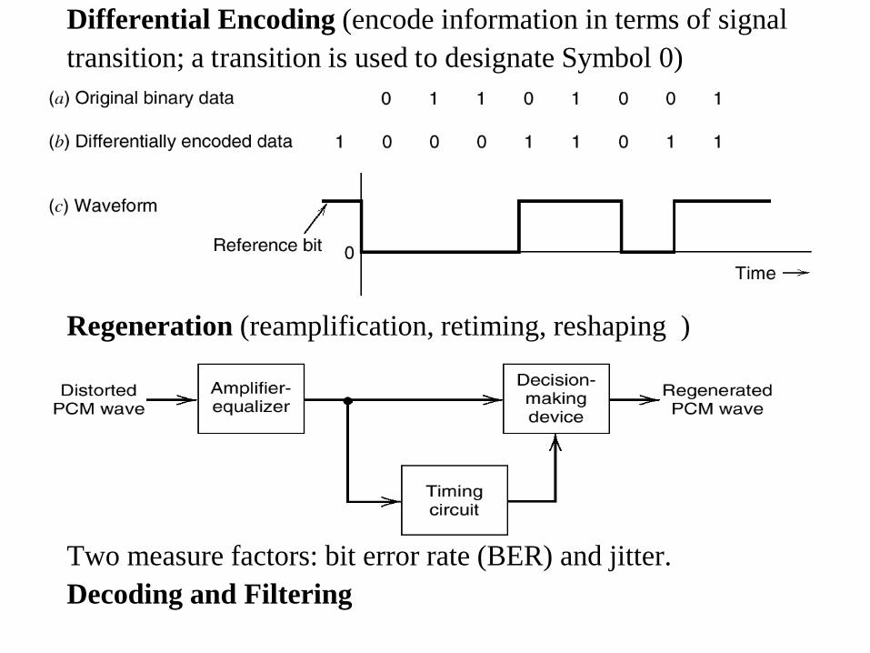
Differential Encoding (encode information in terms of signal transition; a transition is used to designate Symbol 0)

Regeneration (reamplification, retiming, reshaping )

Two measure factors: bit error rate (BER) and jitter. Decoding and Filtering

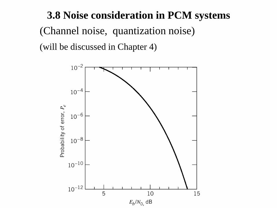
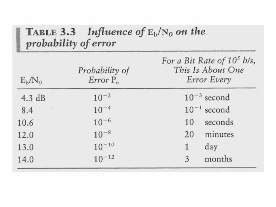
3.8 Noise consideration in PCM systems (Channel noise, quantization noise) (will be discussed in Chapter 4)

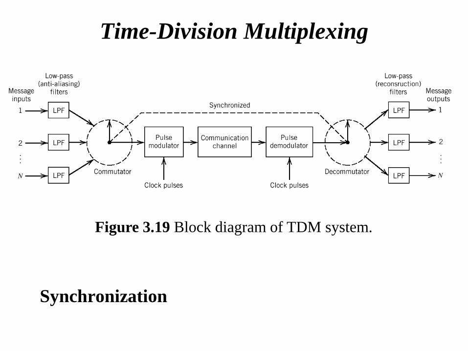
Time-Division Multiplexing

Synchronization

Figure 3.19 Block diagram of TDM system.

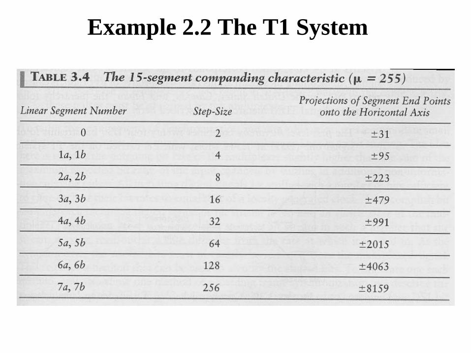
Example 2.2 The T1 System

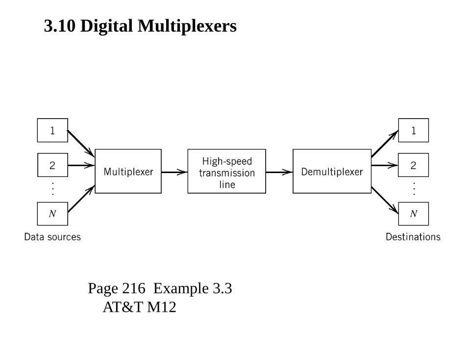
3.10 Digital Multiplexers

Page 216 Example 3.3 AT&T M12

3.11 Virtues, Limitations and Modifications of PCM

Advantages of PCM

1. Robustness to noise and interference

2. Efficient regeneration

3. Efficient SNR and bandwidth trade-off

4. Uniform format

5. Ease add and drop

6. Secure

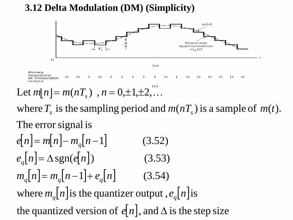
3.12 Delta Modulation (DM) (Simplicity)

[ ]

[ ] [ ] [ ][ ] [ ][ ] [ ] [ ]

[ ] [ ][ ] size step theis and , of version quantized the

is ,output quantizer theis where

(3.54) 1

(3.53) ) sgn(

(3.52) 1 is signalerror The

).( of sample a is )( and period sampling theis where,2,1,0 , )(Let

∆

+−=

∆=

−−=

±±==

nenenm

nenmnmnenenmnmne

tmnTmTnnTmnm

qq

qqq

q

q

ss

s

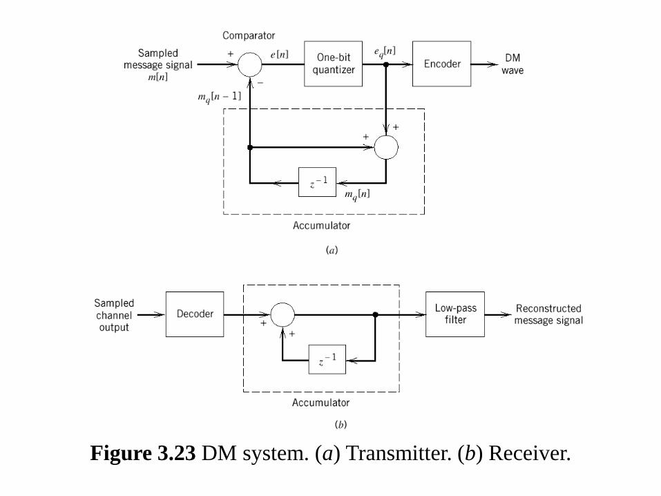
Figure 3.23 DM system. (a) Transmitter. (b) Receiver.

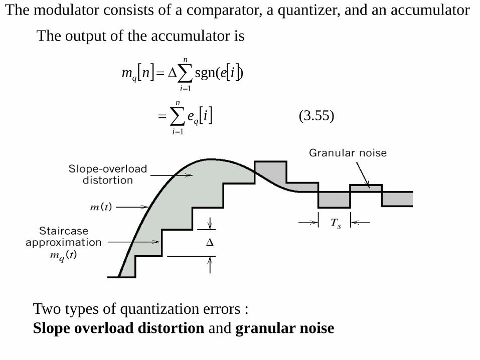
The modulator consists of a comparator, a quantizer, and an accumulator The output of the accumulator is

[ ] [ ]

[ ] (3.55)

)sgn(

1

1

∑

∑

=

=

=

∆=

n

iq

n

iq

ie

ienm

Two types of quantization errors : Slope overload distortion and granular noise

[ ][ ] [ ] [ ]

[ ] [ ] [ ] [ ][ ]

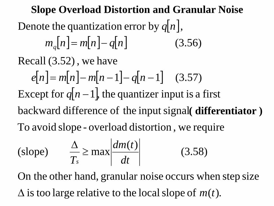
.)( of slope local the torelative large toois size step whenoccurs noisegranular hand,other theOn

(3.58) )(max (slope)

require we, distortion overload-slope avoid Tosignalinput theof difference backward

first a isinput quantizer the,1for Except (3.57) 11

have we, (3.52) Recall(3.56) , by error onquantizati theDenote

tm

dttdm

T

nqnqnmnmne

nqnmnmnq

s

q

∆

≥∆

−−−−−=

−=

Slope Overload Distortion and Granular Noise

( differentiator )

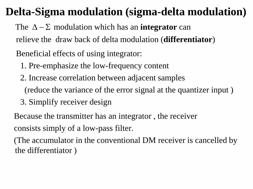
Delta-Sigma modulation (sigma-delta modulation) The modulation which has an integrator can relieve the draw back of delta modulation (differentiator)

Beneficial effects of using integrator: 1. Pre-emphasize the low-frequency content 2. Increase correlation between adjacent samples (reduce the variance of the error signal at the quantizer input ) 3. Simplify receiver design

Because the transmitter has an integrator , the receiver consists simply of a low-pass filter. (The accumulator in the conventional DM receiver is cancelled by

the differentiator )

Σ−∆

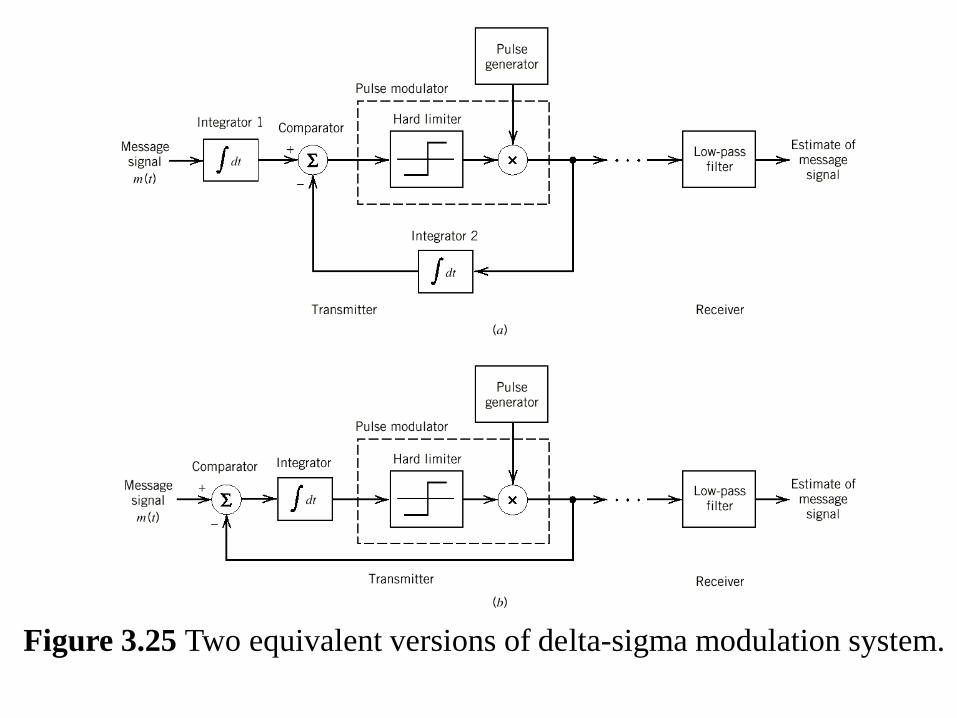
Figure 3.25 Two equivalent versions of delta-sigma modulation system.

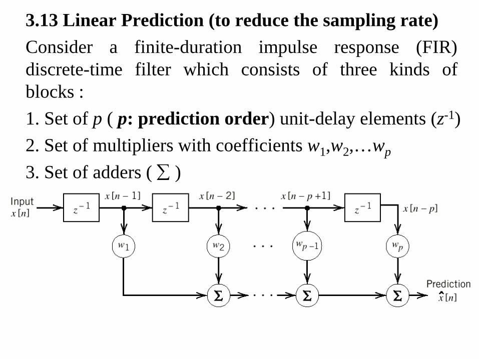
3.13 Linear Prediction (to reduce the sampling rate) Consider a finite-duration impulse response (FIR) discrete-time filter which consists of three kinds of blocks : 1. Set of p ( p: prediction order) unit-delay elements (z-1) 2. Set of multipliers with coefficients w1,w2,…wp

3. Set of adders ( ∑ )

[ ]

[ ] [ ] [ ]

[ ][ ]

[ ][ ] [ ] [ ][ ]

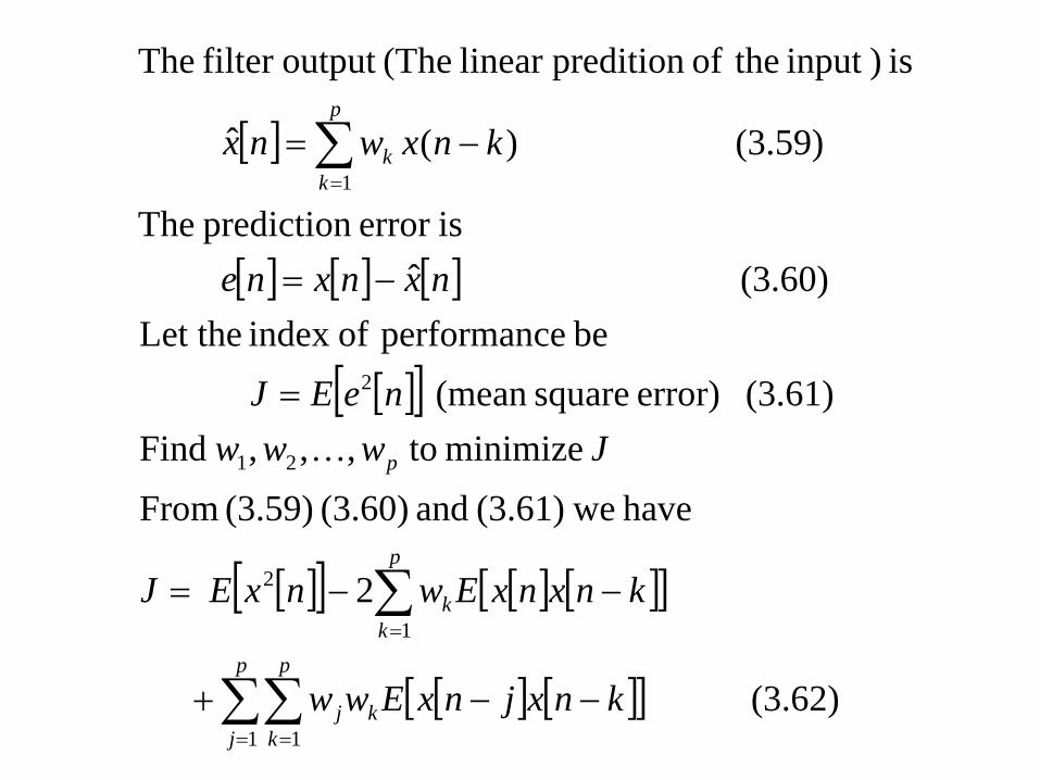
[ ] [ ][ ] (3.62)

2

have we(3.61) and (3.60) (3.59) From minimize to,,, Find

(3.61) error) square (mean be eperformanc ofindex Let the

(3.60) ˆ iserror prediction The

(3.59) )(ˆ

is )input theof preditionlinear (Theoutput filter The

1 1

1

2

21

2

1

∑∑

∑

∑

= =

=

=

−−+

−−=

=

−=

−=

p

j

p

kkj

p

kk

p

p

kk

knxjnxEww

knxnxEwnx EJ

JwwwneEJ

nxnxne

knxwnx

[ ][ ] [ ][ ][ ][ ]

[ ] [ ] [ ][ ]

[ ] [ ]

[ ] [ ]

[ ] [ ] [ ]

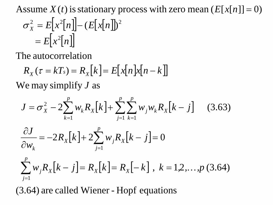
equations Hopf-Wiener called are (3.64)

(3.64) 21 ,

022

(3.63) 2

as simplify may We)(

ationautocorrel The

)( 0)]][[( mean zero withprocess stationary is )( Assume

1

1

1 11

2

2

222

,p,,kkRkRjkRw

jkRwkRwJ

jkRwwkRwJ

JknxnxEkRkTR

nxEnxEnxE

nxEtX

p

jXXXj

p

jXjX

k

p

j

p

kXkj

p

kXkX

XsX

X

=−==−

=−+−=∂∂

−+−=

−===

=

−=

=

∑

∑

∑∑∑

=

=

= ==

σ

τ

σ

[ ]

[ ] [ ] [ ][ ] [ ] [ ]

[ ] [ ] [ ]

[ ] [ ] [ ]

[ ] [ ]

[ ]

2min

1

12

02

1

2

11

2min

210

1

01

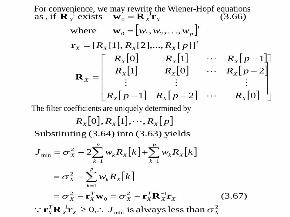
thanless always is 0,

(3.67)

2

yields(3.63) into (3.64) ngSubstituti,, 1, 0

021

201110

]][],...,2[ ],1[[

,,, where

(3.66) exists if , as

XXXTX

XXTXX

TXX

p

kXkX

p

kXk

p

kXkX

XXX

XXX

XXX

XXX

X

TXXXX

Tp

XXX

J

kRw

kRwkRwJ

pRRR

RpRpR

pRRRpRRR

pRRR

www

σσσ

σ

σ

∴≥

−=−=

−=

+−=

−−

−−

=

=

=

=

−

−

=

==

−−

∑

∑∑

rRrrRrwr

R

r

w

rRwR

For convenience, we may rewrite the Wiener-Hopf equations

The filter coefficients are uniquely determined by

[ ] [ ]

[ ] [ ]

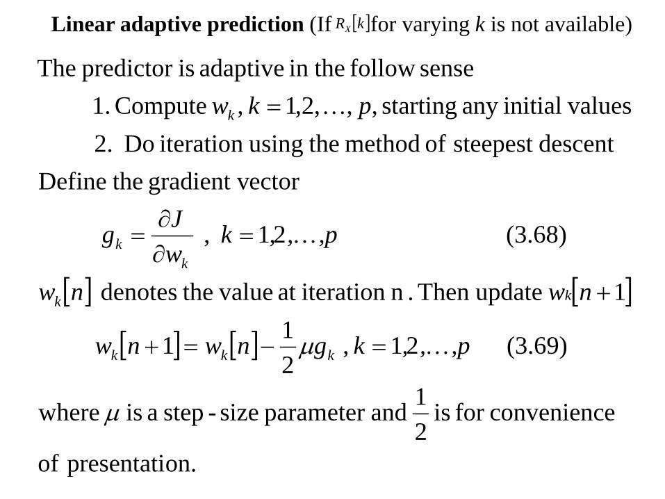
on.presentati of

econveniencfor is 21 andparameter size-stepa is where

(3.69) 21 ,211

1 update Then . n iterationat value thedenotes

(3.68) 21 ,

ectorgradient v theDefinedescentsteepest of method theusing iteration Do2.

valuesinitialany starting ,,,2,1 , Compute 1. sensefollow thein adaptive ispredictor The

µ

µ ,p,,kgnwnw

nwnw

,p,,kwJg

pkw

kkk

kk

kk

k

=−=+

+

=∂∂

=

=

[ ] kRXLinear adaptive prediction (If for varying k is not available)

[ ] [ ]

[ ] [ ][ ] [ ] [ ][ ]

[ ] [ ]

[ ] [ ] [ ] [ ] [ ] [ ]

[ ] [ ] [ ] [ ] [ ] [ ]

[ ] [ ] [ ]

[ ] [ ] [ ] [ ]

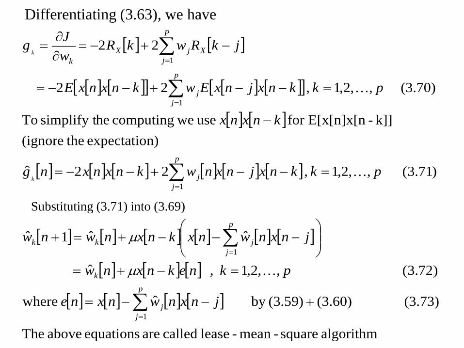
algorithm square-mean-lease called are equations above The

(3.73) (3.60)(3.59)by ˆ where

)72.3( ,,2,1 , ˆ

ˆˆ1ˆ

)71.3( ,,2,1 , 22ˆ

n)expectatio the(ignorek]]-x[nfor E[x[n] use wecomputing hesimplify t To

(3.70) ,,2,1 , 22

22

1

1

1

1

1

+−−=

=−+=

−−−+=+

=−−+−−=

−

=−−+−−=

−+−=∂∂

=

∑

∑

∑

∑

∑

=

=

=

=

=

jnxnwnxne

pkneknxnw

jnxnwnxknxnwnw

pkknxjnxnwknxnxng

knxnx

pkknxjnxEwknxnxE

jkRwkRwJg

p

jj

k

p

jjkk

p

jj

p

jj

P

jXjX

k

k

k

µ

µ

Substituting (3.71) into (3.69)

Differentiating (3.63), we have

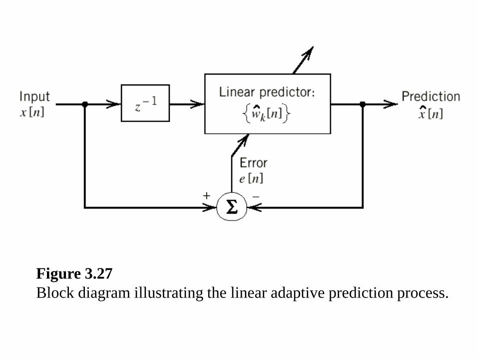
Figure 3.27 Block diagram illustrating the linear adaptive prediction process.

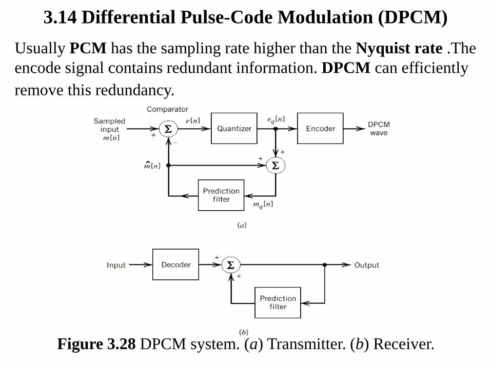
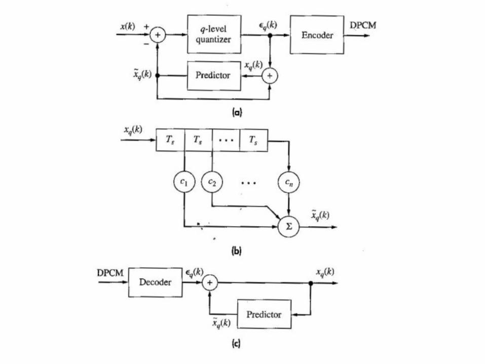
3.14 Differential Pulse-Code Modulation (DPCM) Usually PCM has the sampling rate higher than the Nyquist rate .The encode signal contains redundant information. DPCM can efficiently remove this redundancy.

Figure 3.28 DPCM system. (a) Transmitter. (b) Receiver.

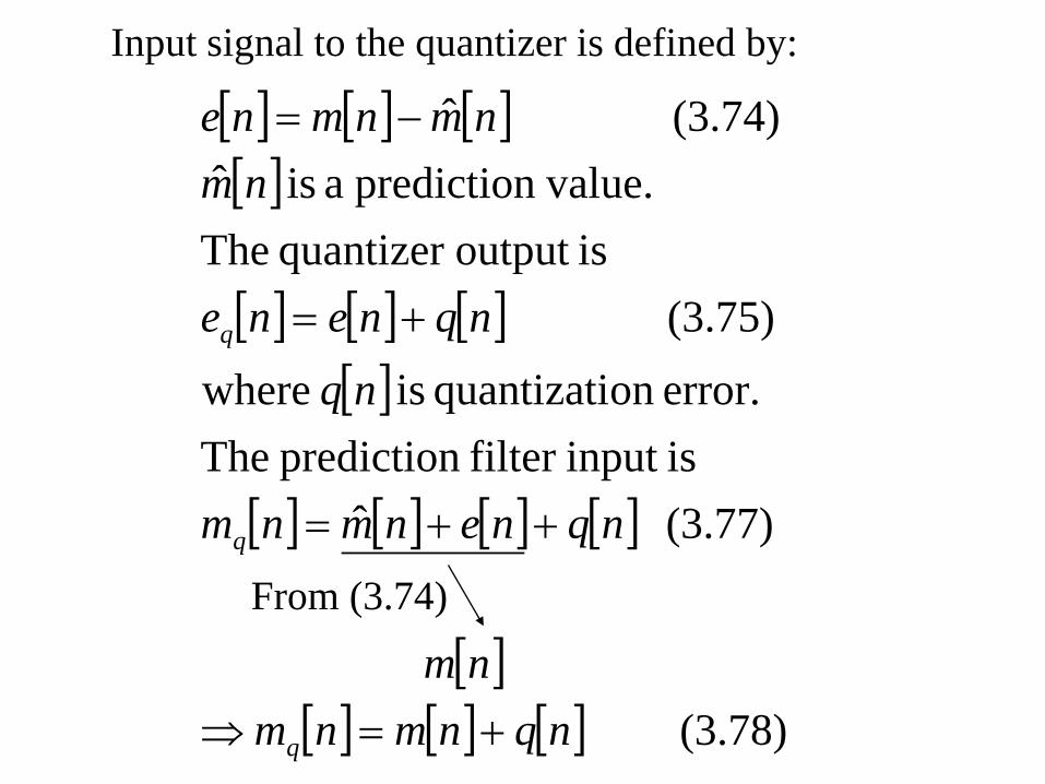
Input signal to the quantizer is defined by:

[ ] [ ] [ ][ ]

[ ] [ ] [ ][ ]

[ ] [ ] [ ] [ ]

[ ][ ] [ ] [ ] (3.78)

(3.77) ˆisinput filter prediction Theerror. onquantizati is where(3.75)

isoutput quantizer The value.predictiona is ˆ(3.74) ˆ

nqnmnmnm

nqnenmnm

nqnqnene

nmnmnmne

q

q

q

+=⇒

++=

+=

−=

From (3.74)

[ ] [ ]

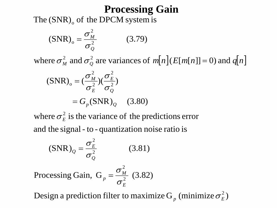
) (minimize G maximize filter to predictiona Design

(3.82) G Gain, Processing

(3.81) )SNR(

is ratio noise onquantizati-to-signal theanderror sprediction theof variance theis where

(3.80))SNR(

))(((SNR)

and 0)]][[( of variancesare and where

(3.79) (SNR)

is system DPCM theof (SNR) The

2

2

2

2

2

2

2

2

2

2

o

22

2

2

o

o

Ep

E

Mp

Q

EQ

E

Qp

Q

E

E

M

QM

Q

M

G

nqnmEnm

σ

σσ

σσ

σ

σσ

σσ

σσ

σσ

=

=

=

=

=

=

Processing Gain

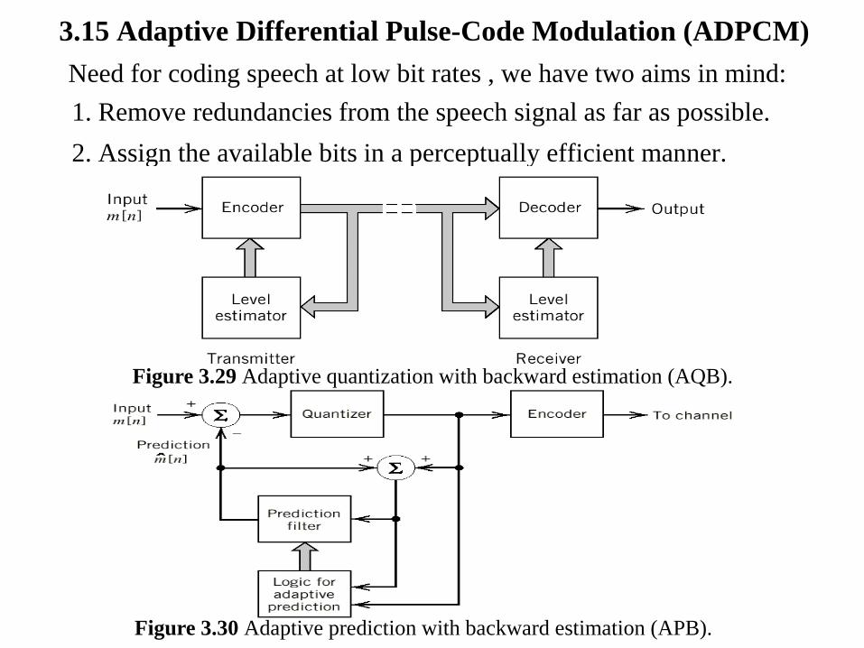
3.15 Adaptive Differential Pulse-Code Modulation (ADPCM) Need for coding speech at low bit rates , we have two aims in mind: 1. Remove redundancies from the speech signal as far as possible. 2. Assign the available bits in a perceptually efficient manner.

Figure 3.29 Adaptive quantization with backward estimation (AQB).

Figure 3.30 Adaptive prediction with backward estimation (APB).

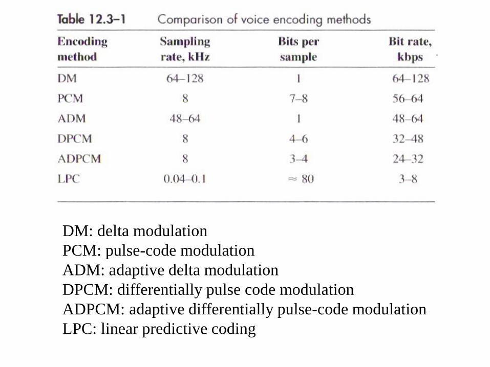
DM: delta modulation PCM: pulse-code modulation ADM: adaptive delta modulation DPCM: differentially pulse code modulation ADPCM: adaptive differentially pulse-code modulation LPC: linear predictive coding

PowerPoint 簡報 - 國立臺灣大學cc.ee.ntu.edu.tw/~wujsh/10101PC/Chapter3_101.11.05.pdfPulse...

Documents

Transcript of PowerPoint 簡報 - 國立臺灣大學cc.ee.ntu.edu.tw/~wujsh/10101PC/Chapter3_101.11.05.pdfPulse...