Pole skipping away from maximal chaosGábor Sárosi (CERN)

Based on 1908.03574 with Mezei

2010.08558 with Choi and Mezei

Plan

1. Introduction: quantum butterfly effect

2. Pole skipping

3. Large q SYK chain

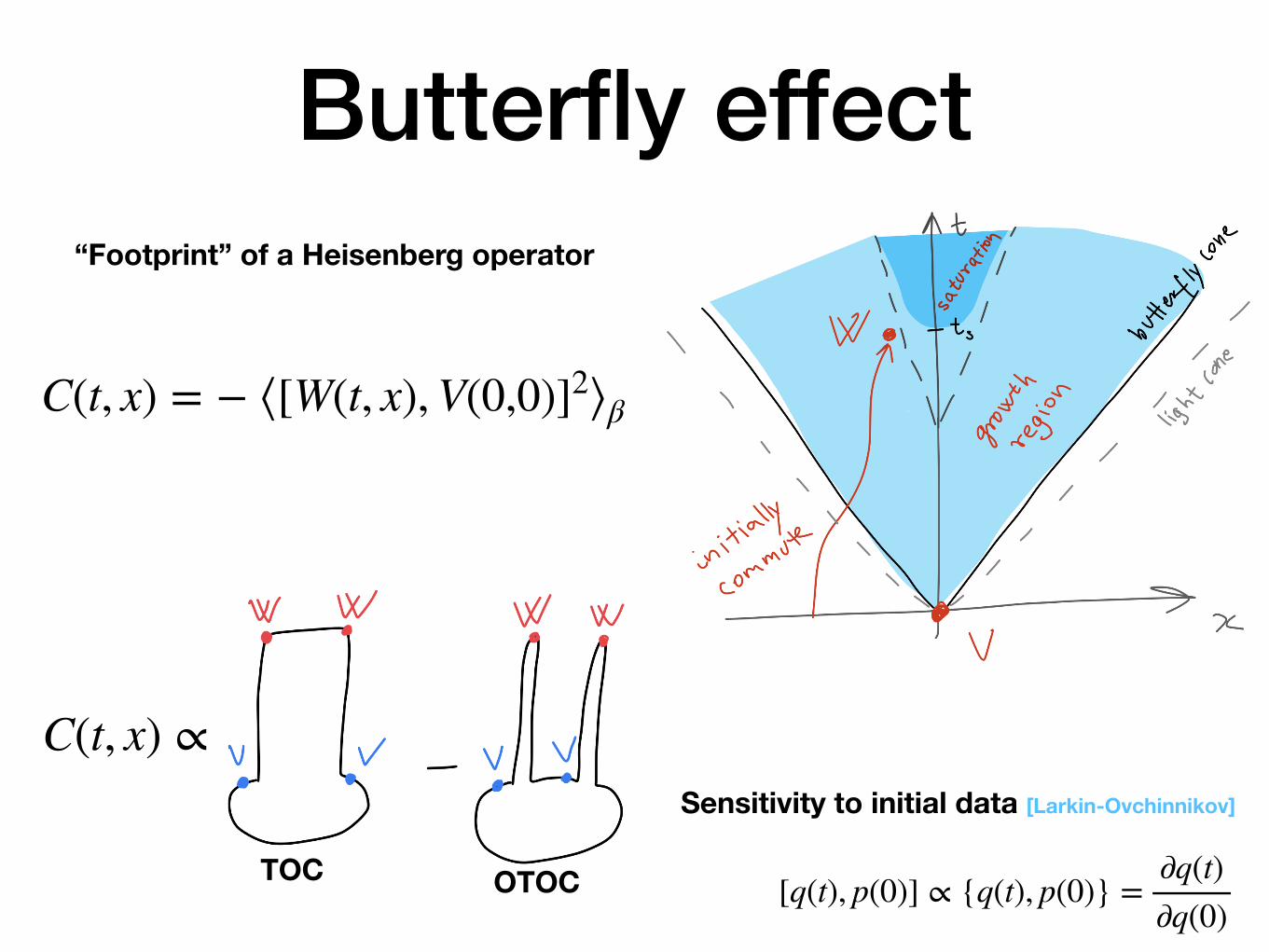
Sensitivity to initial data [Larkin-Ovchinnikov]

[q(t), p(0)] ∝ {q(t), p(0)} =∂q(t)∂q(0)

C(t, x) = − ⟨[W(t, x), V(0,0)]2⟩β

“Footprint” of a Heisenberg operator

C(t, x) ∝

TOC OTOC

Butterfly effect

Butterfly effect

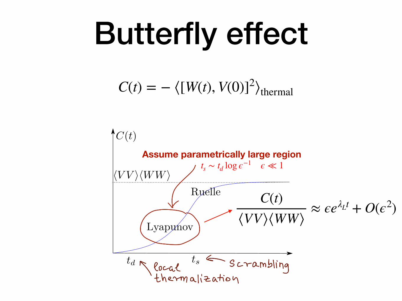
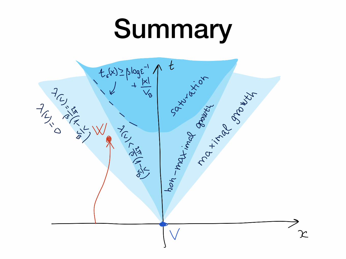
Assume parametrically large regionts ∼ td log ϵ−1 ϵ ≪ 1

C(t) = − ⟨[W(t), V(0)]2⟩thermal

C(t)⟨VV⟩⟨WW⟩

≈ ϵeλLt + O(ϵ2)

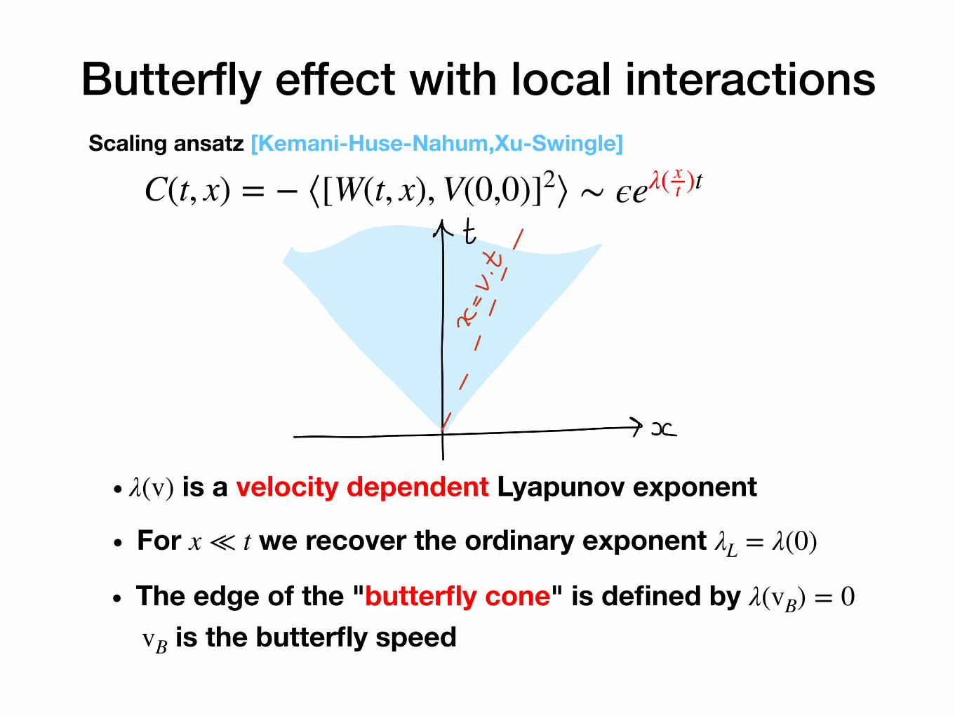
Butterfly effect with local interactionsScaling ansatz [Kemani-Huse-Nahum,Xu-Swingle]

∙ λ(v) is a velocity dependent Lyapunov exponent

∙  For x ≪ t we recover the ordinary exponent λL = λ(0)

∙  The edge of the "butterfly cone" is defined by λ(vB) = 0vB is the butterfly speed

∼ ϵeλ( xt )tC(t, x) = − ⟨[W(t, x), V(0,0)]2⟩

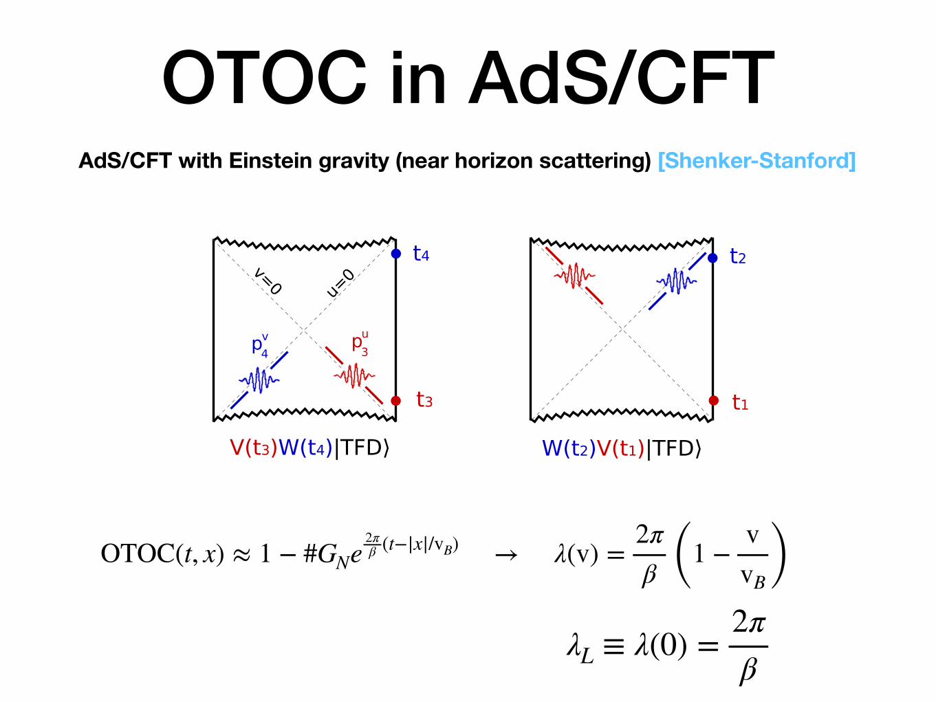
OTOC in AdS/CFTAdS/CFT with Einstein gravity (near horizon scattering) [Shenker-Stanford]

Figure 3: The one-particle state W (t4)|TFDi can be represented on any bulk slice.

panel of Fig. 3. We can represent this one-particle state on di↵erent bulk slices. In order

to act with the V (t3) operator, it is convenient to evolve the state backwards to an early

slice that touches the R boundary at time t3, as shown in the right panel. On this slice,

the W and V quanta are spacelike related, so it is simple to act with the V operator. The

result is an ‘in’ state, as shown in the left panel of Fig. 4.

������������� ��� ���������

��

�� ��

�

��

������

��� �

Figure 4: The correlation function (7) is an inner product of these two states. As explainedin the text, changing the ordering of these operators changes an ‘in’ state to an ‘out’ state.

This ‘in’ state can be described using Klein-Gordon wave functions. These are simply

bulk to boundary propagators from the relevant points on the boundary. In high-energy

scattering processes, it is often useful to describe wave functions in terms of longitudinal

momentum and transverse position. We would therefore like to decompose these Klein

Gordon wave functions in a basis of (pv, x) for the W particle and (pu, x) for the V particle.

In a curved background, the notion of momentum is not unique, so in order to be precise,

we will proceed as follows. First, we represent the W state in the Hilbert space on the

v = 0 surface, and the V state on the u = 0 slice. We then Fourier transform in the

remaining null coordinates, getting the wave functions 3 and 4 from Eq (12) and (13).

9

OTOC(t, x) ≈ 1 − #GNe2πβ (t−|x|/vB) → λ(v) =

2πβ (1 −

vvB )

λL ≡ λ(0) =2πβ

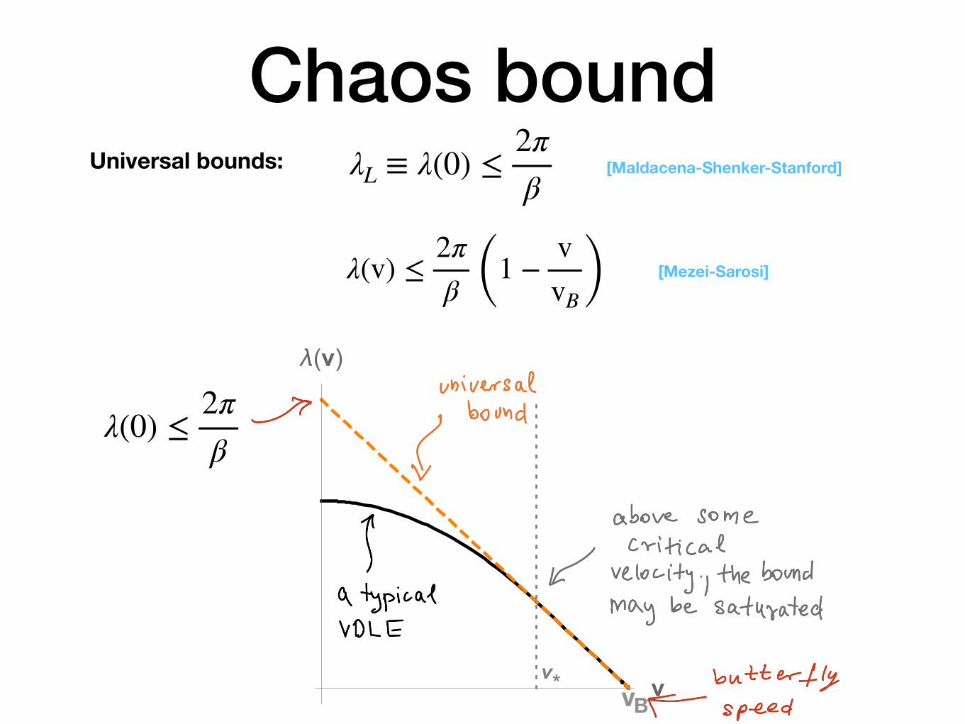
Chaos bound

v* v

�(v)

λ(v) ≤2πβ (1 −

vvB ) [Mezei-Sarosi]

λ(0) ≤2πβ

[Maldacena-Shenker-Stanford]

vB

Universal bounds: λL ≡ λ(0) ≤2πβ

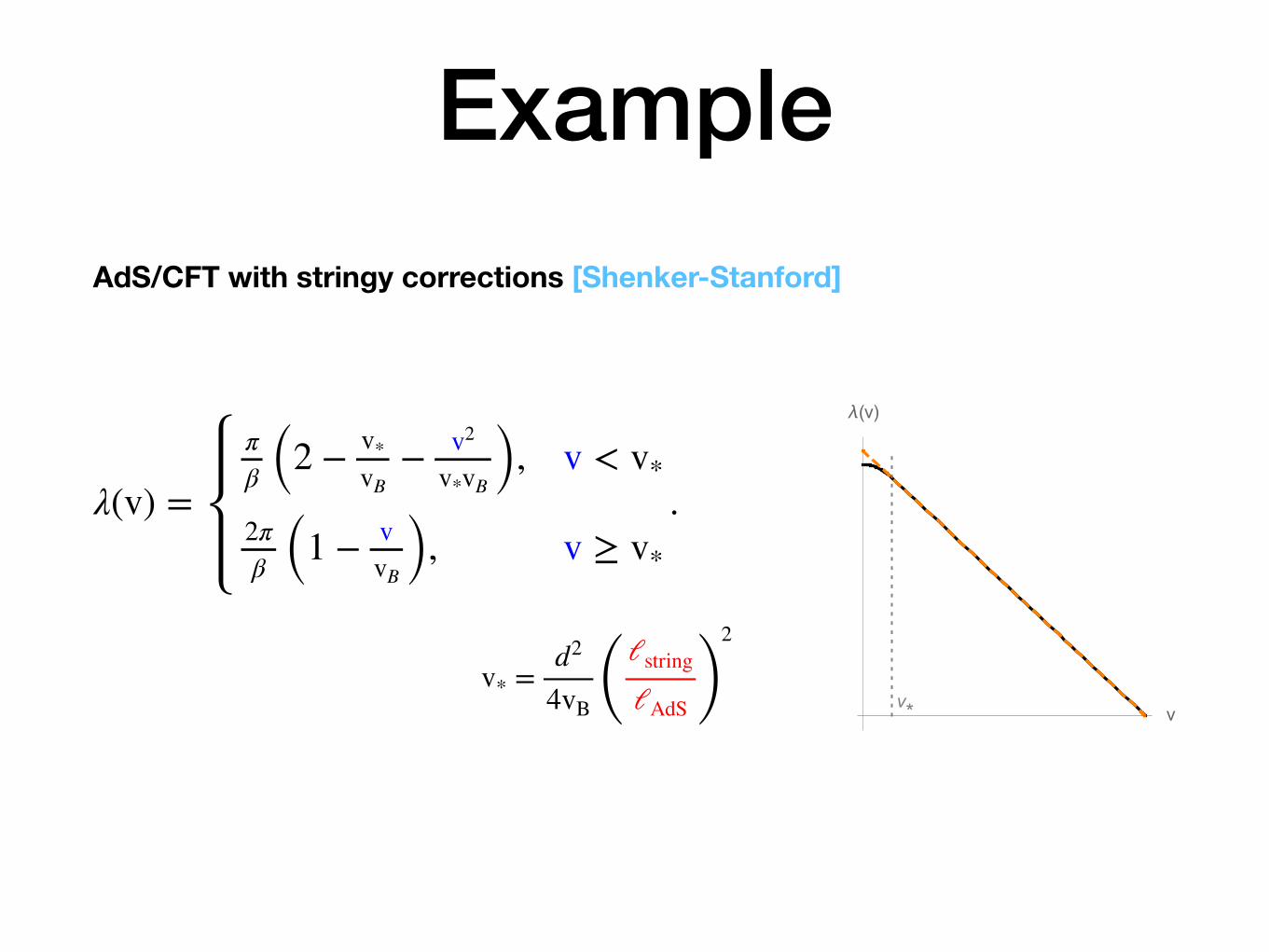
ExampleAdS/CFT with stringy corrections [Shenker-Stanford]

λ(v) =

πβ (2 − v*

vB− v2

v*vB ), v < v*

2πβ (1 − v

vB ), v ≥ v*

.

v* =d2

4vB (ℓstring

ℓAdS )2

v* v

�(v)

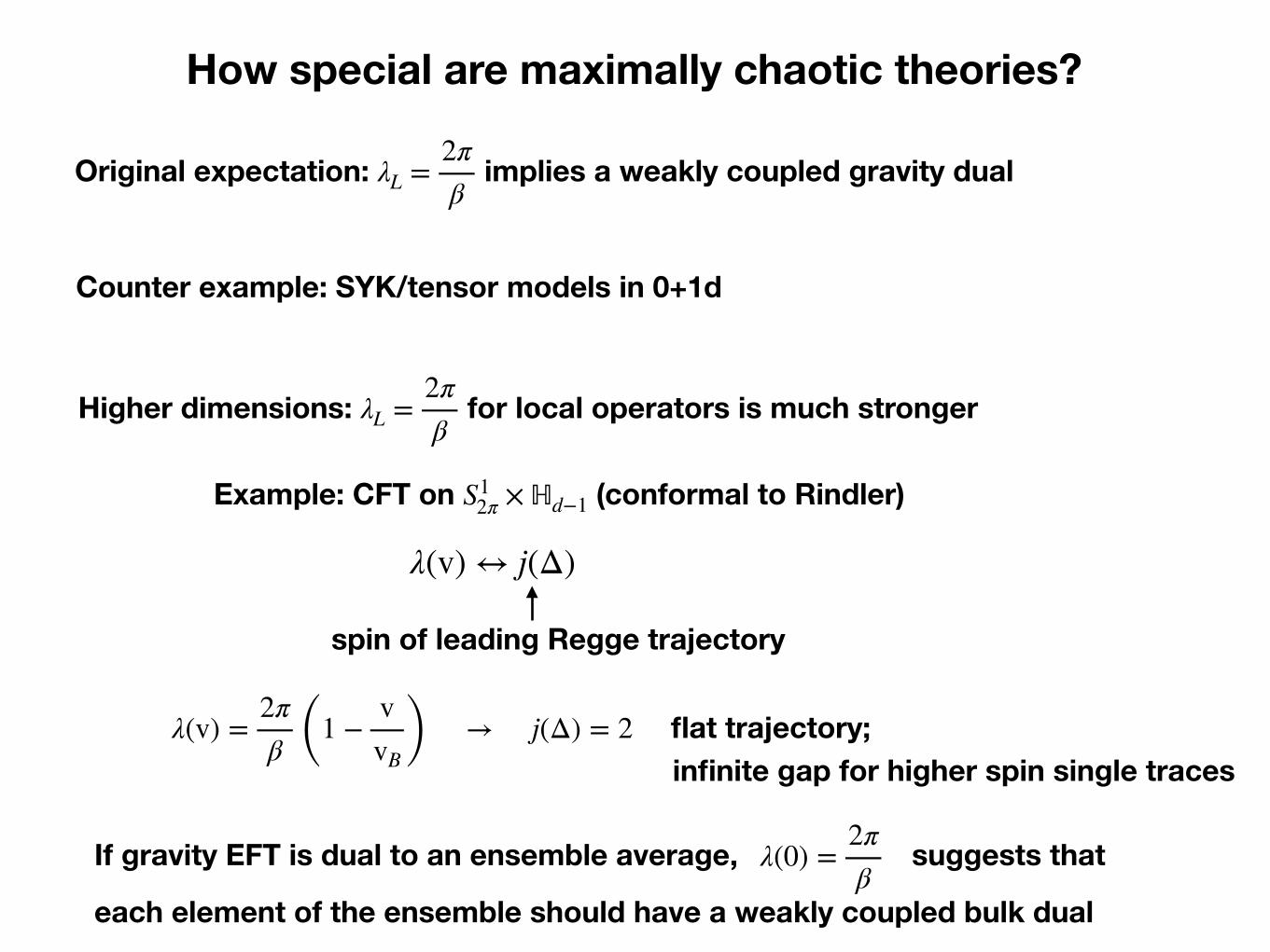
How special are maximally chaotic theories?

Original expectation: λL =2πβ implies a weakly coupled gravity dual

Counter example: SYK/tensor models in 0+1d

Higher dimensions: λL =2πβ for local operators is much stronger

Example: CFT on S12π × ℍd−1 (conformal to Rindler)

λ(v) ↔ j(Δ)

spin of leading Regge trajectory

λ(v) =2πβ (1 −

vvB ) → j(Δ) = 2  flat trajectory;

infinite gap for higher spin single traces

If gravity EFT is dual to an ensemble average, suggests that

each element of the ensemble should have a weakly coupled bulk dual

λ(0) =2πβ

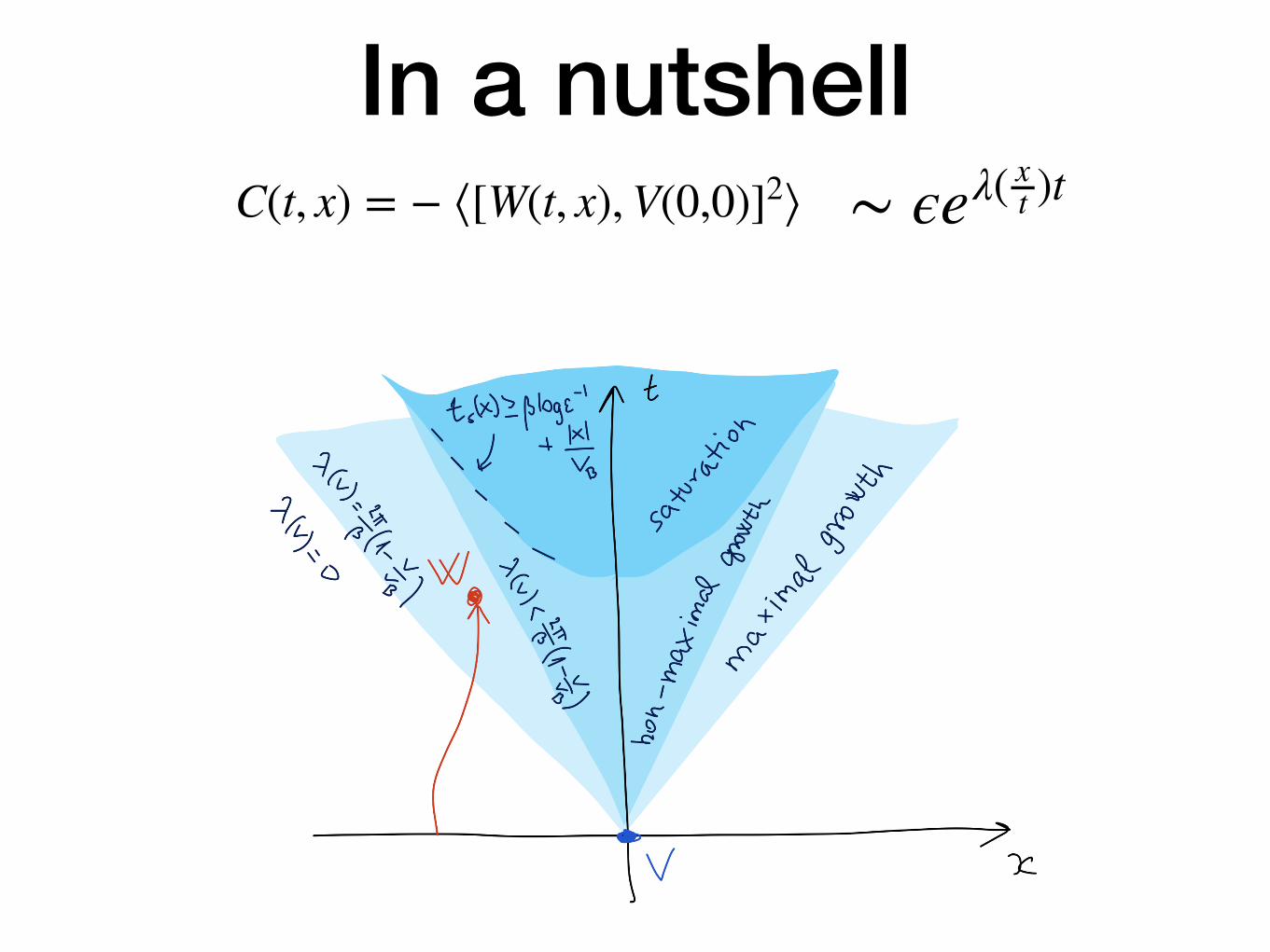
In a nutshellC(t, x) = − ⟨[W(t, x), V(0,0)]2⟩ ∼ ϵeλ( x

t )t

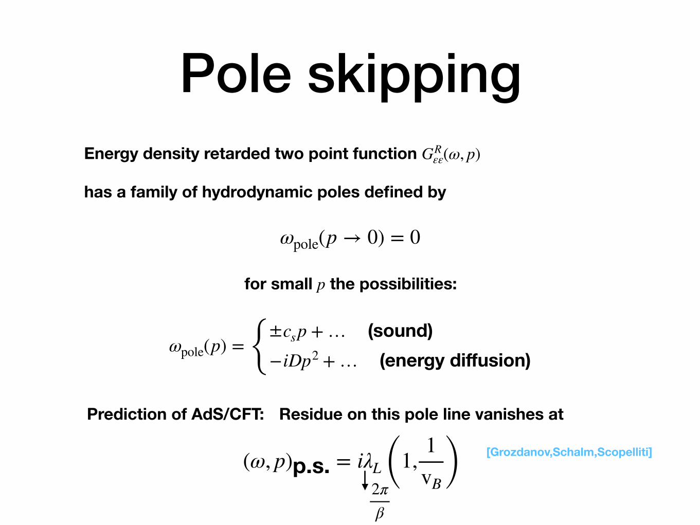
Pole skippingEnergy density retarded two point function GR

εε(ω, p)

has a family of hydrodynamic poles defined by

ωpole(p) = {±csp + … (sound)−iDp2 + … (energy diffusion)

ωpole(p → 0) = 0

for small p the possibilities:

Prediction of AdS/CFT: Residue on this pole line vanishes at

(ω, p)p.s. = iλL (1,1vB ) [Grozdanov,Schalm,Scopelliti]

2πβ

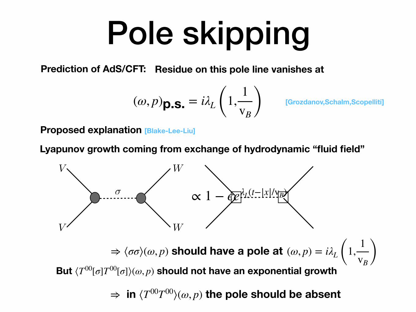
Pole skippingPrediction of AdS/CFT: Residue on this pole line vanishes at

(ω, p)p.s. = iλL (1,1vB ) [Grozdanov,Schalm,Scopelliti]

Proposed explanation [Blake-Lee-Liu]

V

V

W

W

�

V

V

W

W

�

FIG. 3. At leading order in large N correlation functions are controlled by exchange of hydrody-

namic fields �(t). The only di↵erence between time ordered (left) and out-of time-ordered (right)

configurations is in the e↵ective vertex describing the coupling to �(t).

A. To leading order in the limit N ! 1, the scrambling of a generic few-body operator

in a chaotic system allows a coarse-grained description in which the growth of the

operator can be understood as building up a “cloud” of some e↵ective field �. More

explicitly, as indicated in Fig. 2, V (t) can be represented by a core operator V̂ (t),

which involves the degrees of freedom originally in V , dressed by a variable �(t).

B. The chaotic behavior (1.5)–(1.8) of OTOCs can be understood from exchanging and

propagation of � (see Fig. 3).

In this paper we will realise the above elements through developing a “quantum hydrody-

namic” theory for chaos in which we identify � with the hydrodynamic mode for energy

conservation. As we will shortly discuss, this connection between the e↵ective chaos mode

and hydrodynamics can be motivated from the explicit calculations of OTOCs in holography

and SYK models. Our general hydrodynamic theory not only provides a system-independent

explanation of the chaotic behavior (1.5)–(1.8) of OTOCs, but also leads to new predictions

which can be explicitly checked. As we will remark later in the paper, likely the full content

of this hydrodynamic theory only applies to systems which are maximally (or nearly max-

imally) chaotic. Nevertheless, we expect that various features associated with items A and

B above may also apply to non-maximal chaotic systems. So throughout the paper we use

a general Lyapunov exponent � unless explicitly stated.

6

Lyapunov growth coming from exchange of hydrodynamic “fluid field”

∝ 1 − ϵeλL(t−|x|/vB)

⇒ ⟨σσ⟩(ω, p) should have a pole at (ω, p) = iλL (1,1vB )

But ⟨T00[σ]T00[σ]⟩(ω, p) should not have an exponential growth

⇒  in ⟨T00T00⟩(ω, p) the pole should be absent 

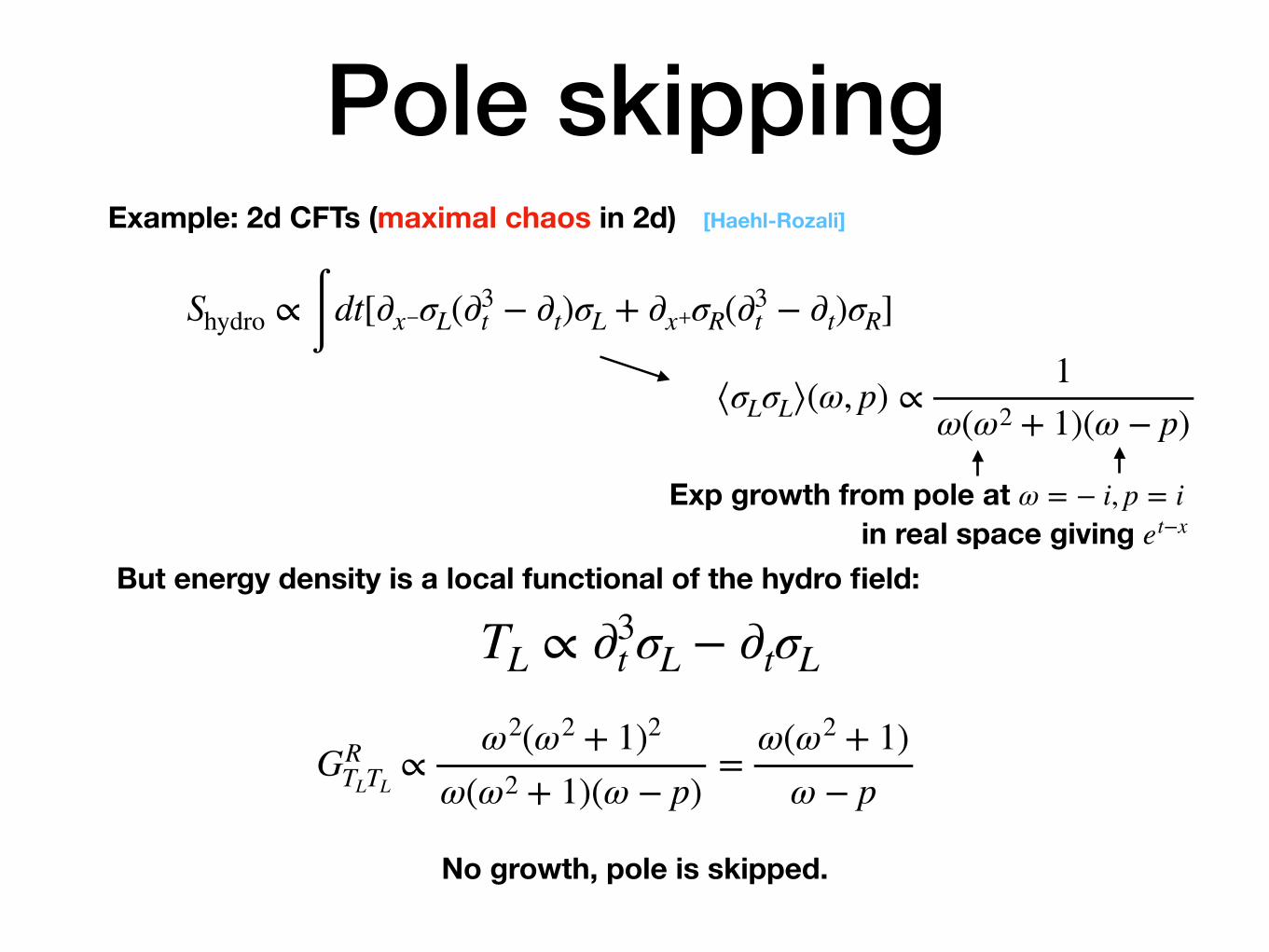
Pole skippingExample: 2d CFTs (maximal chaos in 2d)

Shydro ∝ ∫ dt[∂x−σL(∂3t − ∂t)σL + ∂x+σR(∂3

t − ∂t)σR]

⟨σLσL⟩(ω, p) ∝1

ω(ω2 + 1)(ω − p)

But energy density is a local functional of the hydro field:

TL ∝ ∂3t σL − ∂tσL

GRTLTL

∝ω2(ω2 + 1)2

ω(ω2 + 1)(ω − p)=

ω(ω2 + 1)ω − p

No growth, pole is skipped.

[Haehl-Rozali]

Exp growth from pole at ω = − i, p = iin real space giving et−x

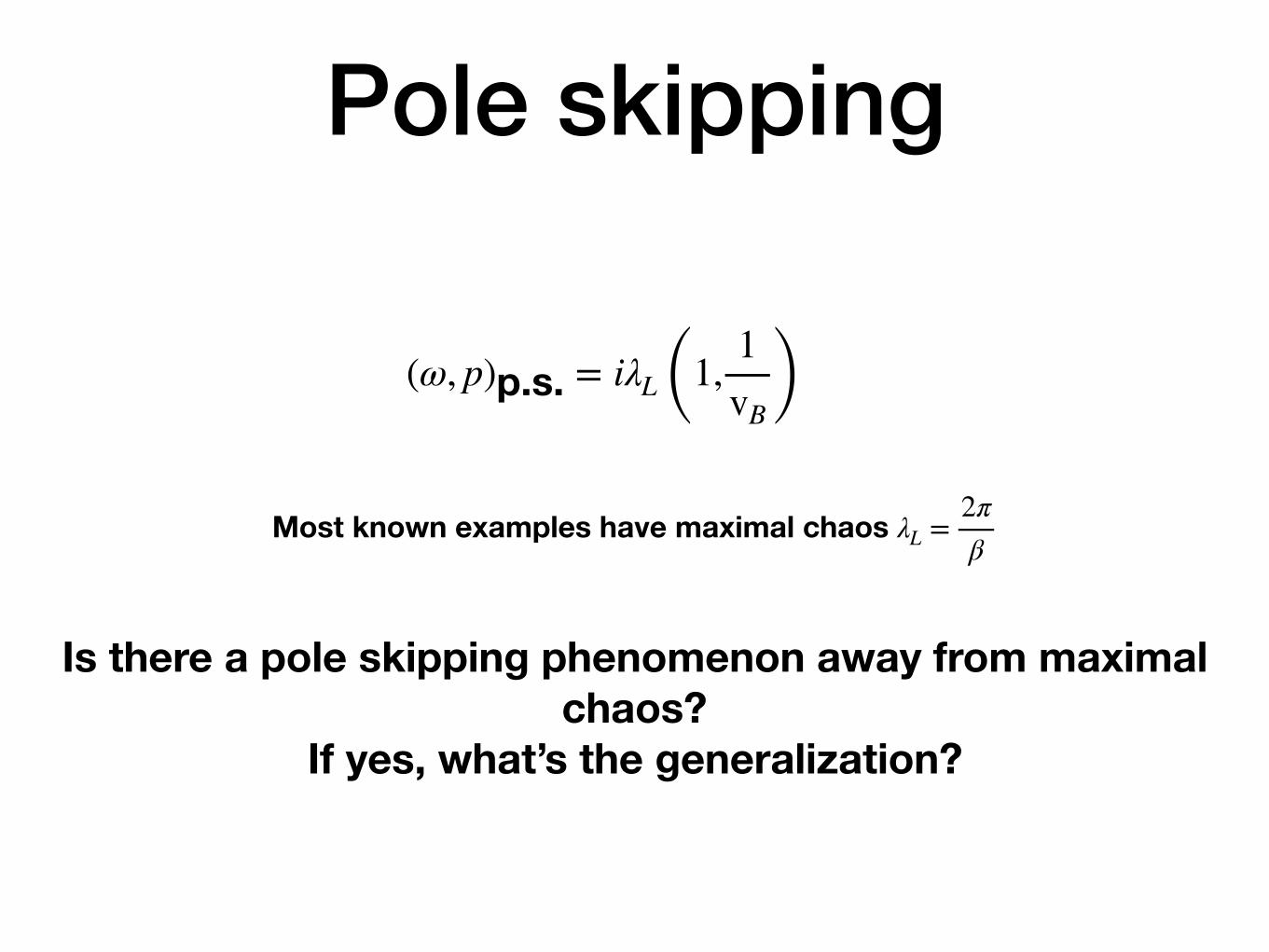
Pole skipping

(ω, p)p.s. = iλL (1,1vB )

Most known examples have maximal chaos λL =2πβ

Is there a pole skipping phenomenon away from maximal chaos?

If yes, what’s the generalization?

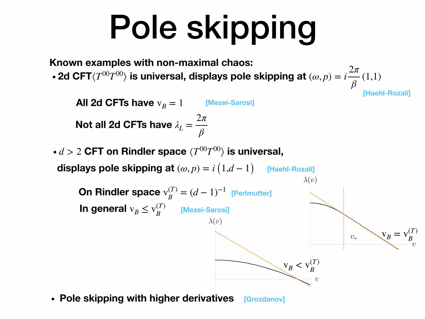
Pole skippingKnown examples with non-maximal chaos:∙ 2d CFT⟨T00T00⟩ is universal, displays pole skipping at (ω, p) = i

2πβ

(1,1)[Haehl-Rozali]

All 2d CFTs have vB = 1

Not all 2d CFTs have λL =2πβ

[Mezei-Sarosi]

∙ d > 2 CFT on Rindler space ⟨T00T00⟩ is universal,[Haehl-Rozali]

On Rindler space v(T )B = (d − 1)−1 [Perlmutter]

displays pole skipping at (ω, p) = i (1,d − 1)

In general vB ≤ v(T )B [Mezei-Sarosi]

vB = v(T )B

vB < v(T )B

∙  Pole skipping with higher derivatives [Grozdanov]

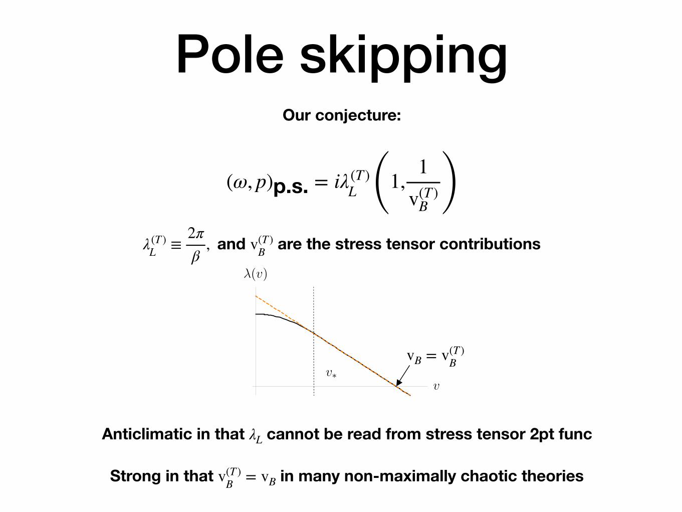
Pole skippingOur conjecture:

(ω, p)p.s. = iλ(T)L (1,

1v(T)

B )λ(T )

L ≡2πβ

,  and v(T )B  are the stress tensor contributions

Anticlimatic in that λL cannot be read from stress tensor 2pt func

Strong in that v(T )B = vB in many non-maximally chaotic theories

vB = v(T )B

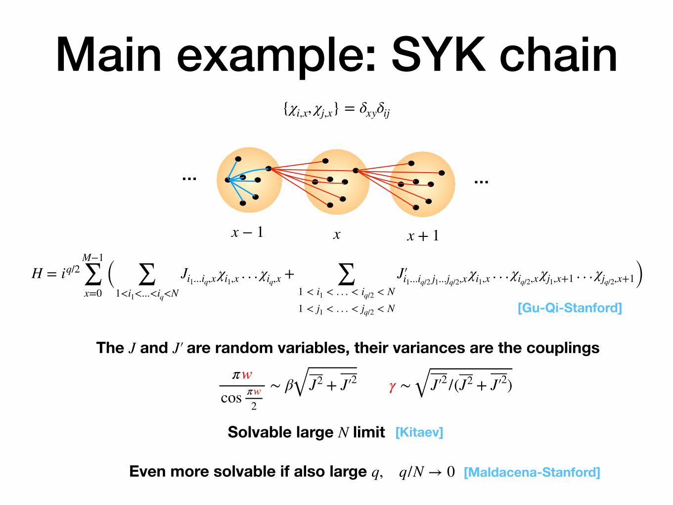
Main example: SYK chain

H = iq/2M−1

∑x=0

( ∑1<i1<...<iq<N

Ji1...iq,x χi1,x . . . χiq,x + ∑1 < i1 < . . . < iq/2 < N1 < j1 < . . . < jq/2 < N

J′ i1...iq/2 j1...jq/2,x χi1,x . . . χiq/2,x χj1,x+1 . . . χjq/2,x+1)

… …

{χi,x, χj,x} = δxyδij

x x + 1x − 1

Solvable large N limit [Kitaev]

Even more solvable if also large q, q/N → 0 [Maldacena-Stanford]

[Gu-Qi-Stanford]

The J and J′  are random variables, their variances are the couplingsπw

cos πw2

∼ β J2 + J′ 2 γ ∼ J′

2 /(J2 + J′ 2)

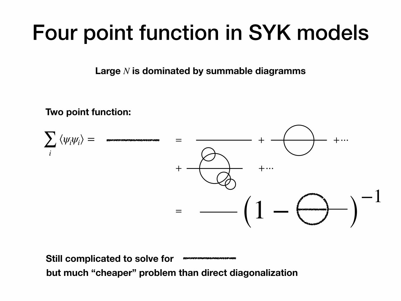
Four point function in SYK models

Two point function:

∑i

⟨ψiψi⟩ = = +

+

+⋯

+⋯

Large N is dominated by summable diagramms

= (1 − )−1

Still complicated to solve for but much “cheaper” problem than direct diagonalization

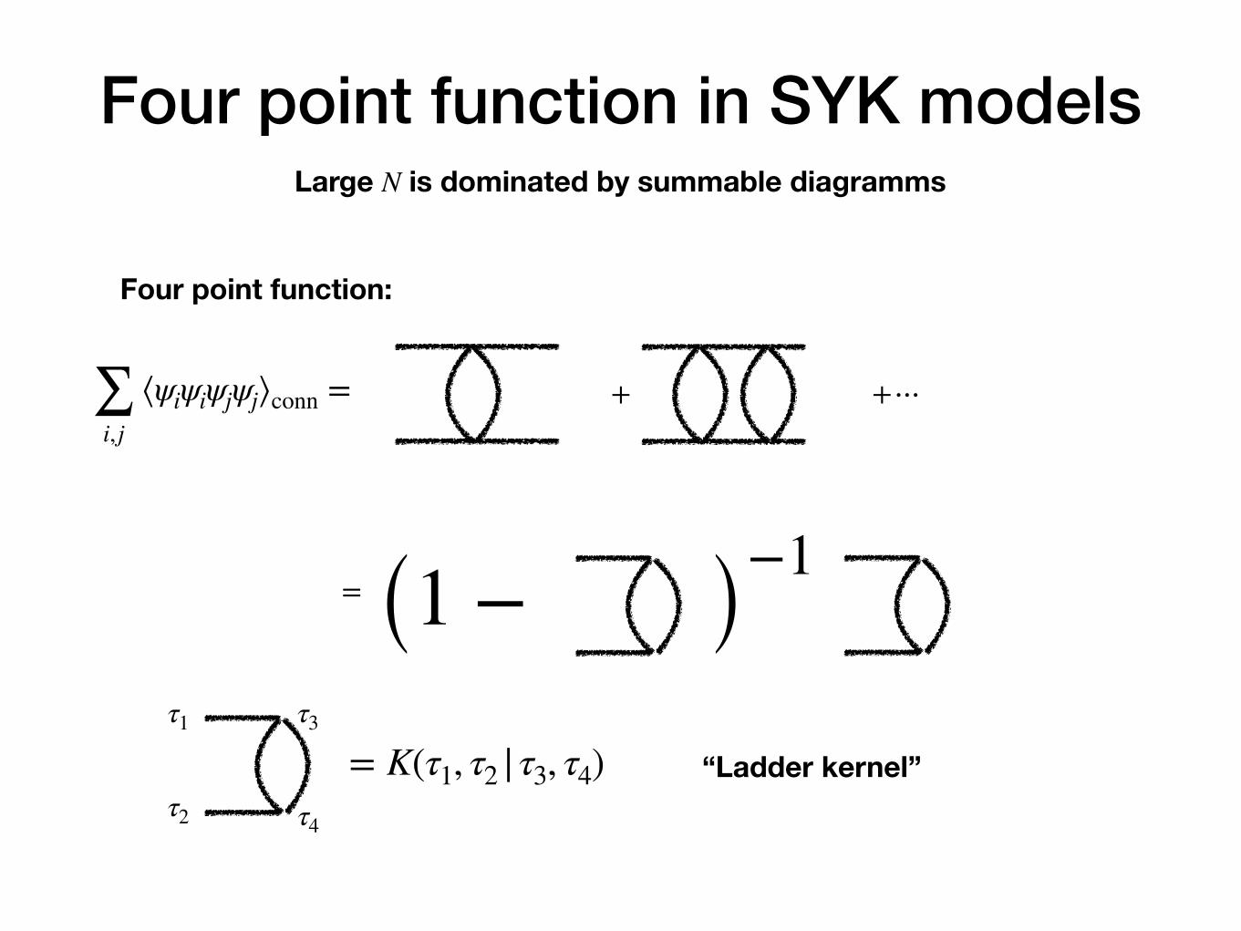
Four point function in SYK models

Four point function:

∑i,j

⟨ψiψiψjψj⟩conn =

Large N is dominated by summable diagramms

+ +⋯

= (1 − )−1

= K(τ1, τ2 |τ3, τ4) “Ladder kernel”

τ1

τ2

τ3

τ4

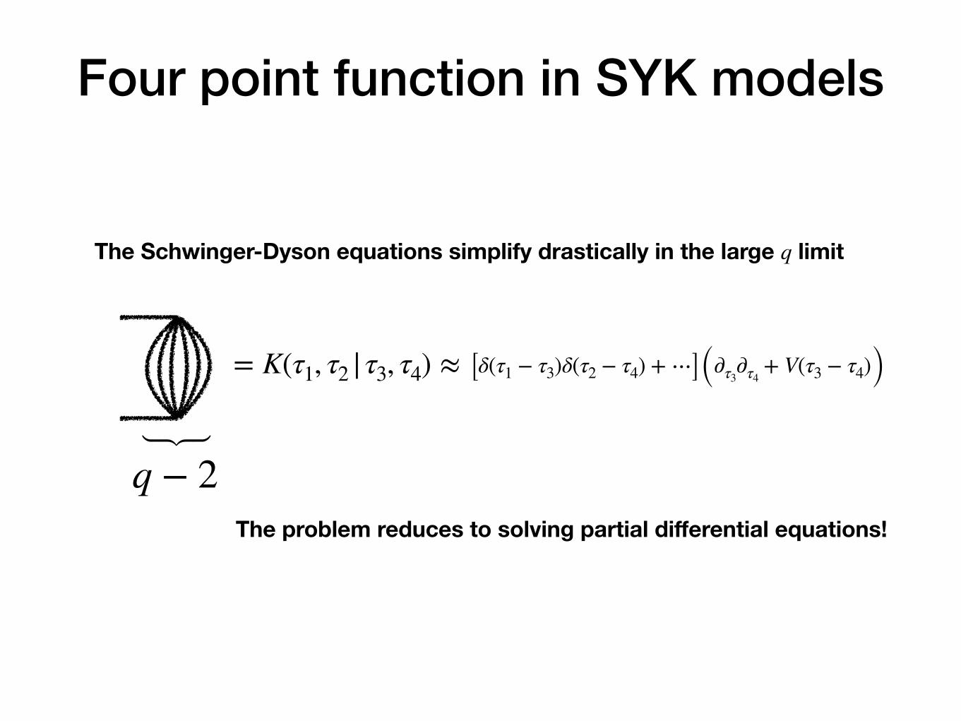
Four point function in SYK models

= K(τ1, τ2 |τ3, τ4) ≈

The Schwinger-Dyson equations simplify drastically in the large q limit

[δ(τ1 − τ3)δ(τ2 − τ4) + ⋯](∂τ3∂τ4

+ V(τ3 − τ4))

forthegrou

ndstateen

ergy

�2of

�v2@2 ⇠�

h(h

�1)v2

cosh

2(⇠)

� (⇠)=

�2 (⇠)

(3.1)

Thegrou

ndstatewavefunctionof

this

problem

is (⇠)⇠

1(cosh

⇠)h

�1,an

dthecorrespon

ding

grou

ndstateen

ergy

givesrise

totheLya

punov

expon

ent

(p)=

(h�1)v,

(3.2)

[MM

:W

esh

ould

compare

this

toGQS!]wherethemom

entum

dep

enden

ceof

hisdefi

ned

viatakingthe1

h

2branch

of(2.15).Thegrow

ingpiece

ofthefourpoint

functionin

real

latticespacex

isthen

represented

byan

integral

oftheform

(heret=

i(Y

�Y

0 )=

i(⌧ 1

+⌧ 2

�⌧ 3

�⌧ 4)/2)

Zdp

1

cos⇣⇡(p)

2

⌘e

(p)t+ipx,

(3.3)

wherewehaveusedthat

theladder

identity

of[22]

relatingtheprefactor

totheexpon

ent.

For

larget,

this

integral

iseither

dom

inated

byasaddle

point

orapoleat(p)=

1,dep

ending

onx.This

mechan

ism

isqu

itegeneric

[4,6,

14,15

,22

,23

],an

das

explained

in[6],lead

s

tothevelocity

dep

endentLya

punov

expon

ent(w

euse

uforvelocity

toavoidconfusion

with

SYK

couplingv)

�(u)=

8 < :�saddle(u)⌘

ext r((ir)

�ru

)when

u<

u⇤

1�

u

u(T

)B

when

u>

u⇤,

(3.4)

wherethestress

tensorbutterflyspeedu(T

)B

andcritical

velocity

u⇤aredefi

ned

viasolving

i

u(T

)B

!=

1,

u⇤=

id(p)

dp

� � � � p=i/u(T

)B

.(3.5)

Exp

licitexpressionsforthesequ

antities

read

as

u(T

)B

=

✓arccosh1+

v+(�

�2)v2

�v2

◆�1

,u⇤=

p(1

+v�2v

2)(1+

v+2(��1)v2)

2+

v.

(3.6)

–11

–

q − 2The problem reduces to solving partial differential equations!

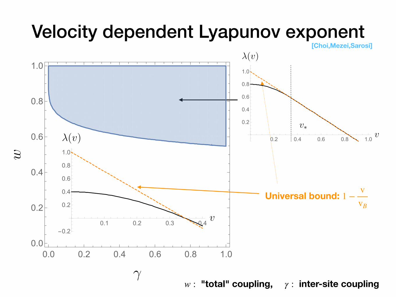
Velocity dependent Lyapunov exponent

w :  "total" coupling,  γ :  inter-site coupling

Universal bound: 1 −vvB

[Choi,Mezei,Sarosi]

0.1 0.2 0.3 0.4-0.2

0.2

0.4

0.6

0.8

1.0

0.2 0.4 0.6 0.8 1.0

0.2

0.4

0.6

0.8

1.0

0.0 0.2 0.4 0.6 0.8 1.00.0

0.2

0.4

0.6

0.8

1.0

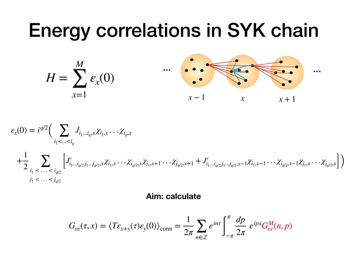
Energy correlations in SYK chain… …

x x + 1x − 1

H =M

∑x=1

εx(0)

εx(0) = iq/2( ∑i1<...<iq

Ji1...iq,x χi1,x . . . χiq,x

+12 ∑

i1 < . . . < iq/2

j1 < . . . < jq/2

[J′ i1...iq/2 j1...jq/2,x χi1,x . . . χiq/2,x χj1,x+1 . . . χjq/2,x+1 + J′ i1...iq/2 j1...jq/2,x−1χi1,x−1 . . . χiq/2,x−1χj1,x . . . χjq/2,x])

Gεε(τ, x) = ⟨Tεx+y(τ)εy(0)⟩conn =1

2π ∑n∈ℤ

einτ ∫π

−π

dp2π

eipxGMεε(n, p)

Aim: calculate

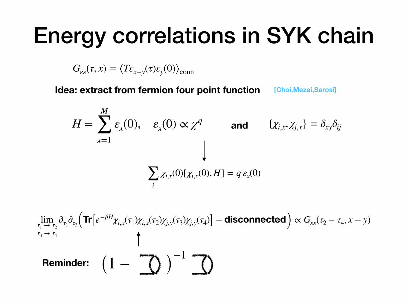
Energy correlations in SYK chainGεε(τ, x) = ⟨Tεx+y(τ)εy(0)⟩conn

Idea: extract from fermion four point function

∑i

χi,x(0)[χi,x(0), H] = q εx(0)

H =M

∑x=1

εx(0), εx(0) ∝ χq {χi,x, χj,x} = δxyδijand

limτ1 → τ2τ3 → τ4

∂τ1∂τ3(Tr[e−βHχi,x(τ1)χi,x(τ2)χj,y(τ3)χj,y(τ4)] − disconnected) ∝ Gεε(τ2 − τ4, x − y)

Reminder: (1 − )−1

[Choi,Mezei,Sarosi]

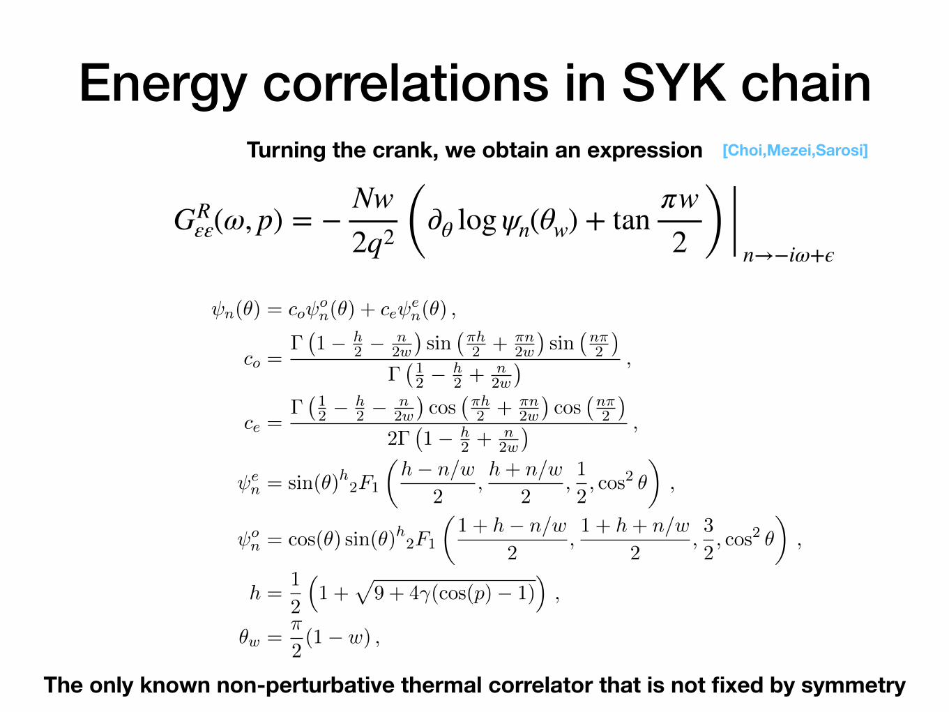
Energy correlations in SYK chain

GRεε(ω, p) = −

Nw2q2 (∂θ log ψn(θw) + tan

πw2 )

n→−iω+ϵ

Turning the crank, we obtain an expression [Choi,Mezei,Sarosi]

n(✓) = co o

n(✓) + ce e

n(✓) ,

co =��1� h

2 � n

2w

�sin

�⇡h

2 + ⇡n

2w

�sin

�n⇡

2

�

��12 � h

2 + n

2w

� ,

ce =��12 � h

2 � n

2w

�cos

�⇡h

2 + ⇡n

2w

�cos

�n⇡

2

�

2��1� h

2 + n

2w

� ,

e

n = sin(✓)h2F1

✓h� n/w

2,h+ n/w

2,1

2, cos2 ✓

◆,

o

n = cos(✓) sin(✓)h2F1

✓1 + h� n/w

2,1 + h+ n/w

2,3

2, cos2 ✓

◆,

h =1

2

⇣1 +

p9 + 4�(cos(p)� 1)

⌘,

✓w =⇡

2(1� w) ,

(1.10)

1.4 Outline

The outline of the paper is as follows. In Sec. 2 we review the SYK chain and its large-q limit,

where the quantum many-body problem can be reduced to solving di↵erential equations. In

Sec. 3 we use the retarded kernel approach for computing �(u). This is considerably simpler

than computing the full four point function that we undertake in Sec. 4. In Sec. 5 we extract

a simple formula for the Euclidean energy density two point function from the complicated

formula for the four point function by taking an OPE limit.

2 Large-q SYK chain

We will be studying the SYK chain introduced in [17], which is a 1+1 dimensional general-

ization of the SYK dot [18–20]. The Hamiltonian of the system is given by

H = iq/2M�1X

x=0

⇣ X

1<i1<...<iq<N

Ji1...iq ,x�i1,x...�iq ,x

+X

1<i1<...<iq/2<N

1<j1<...<jq/2<N

J 0i1...iq/2j1...jq/2,x

�i1,x...�iq/2,x�j1,x+1...�jq/2,x+1

⌘.

(2.1)

Here, �i,x, i = 1, ..., N are Majorana fermions obeying the commutation relation {�i,x,�j,x} =

�xy�ij and periodic boundary condition, �i,0 = �i,M . q is an even integer, and the first line

of (2.1) is an on-site term, while the second line is an interaction between two groups of q/2

fermions on neighboring sites. Ji1...iq ,x, J0i1...iq/2j1...jq/2,x

are independent Gaussian random

– 7 –

The only known non-perturbative thermal correlator that is not fixed by symmetry

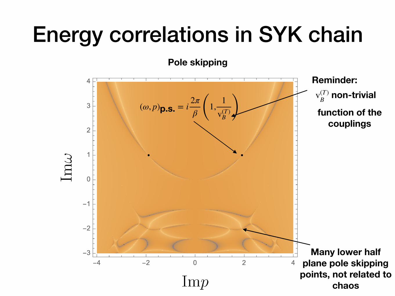
Energy correlations in SYK chainPole skipping

(ω, p)p.s. = i2πβ (1,

1v(T )

B )Reminder: v(T )

B  non-trivial

function of thecouplings

Many lower halfplane pole skipping

points, not related tochaos

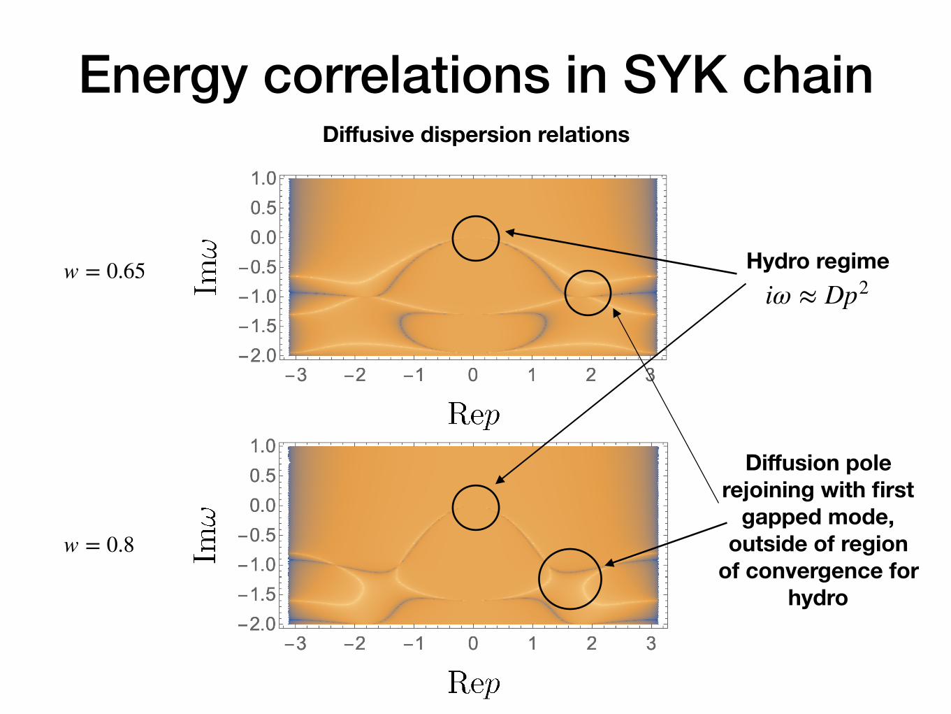
Energy correlations in SYK chainDiffusive dispersion relations

Hydro regimeiω ≈ Dp2

w = 0.65

w = 0.8

Diffusion pole rejoining with first

gapped mode,outside of region

of convergence for hydro

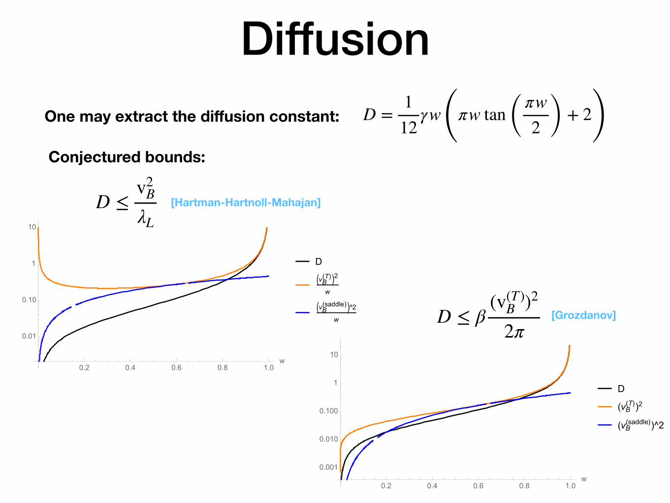
D =112

γw (πw tan ( πw2 ) + 2)

DiffusionOne may extract the diffusion constant:

Conjectured bounds:

D ≤v2

B

λL[Hartman-Hartnoll-Mahajan]

[Grozdanov]D ≤ β(v(T)

B )2

2π

0.2 0.4 0.6 0.8 1.0w

0.001

0.010

0.100

1

10

D

(vB(T))2

(vB(saddle))^2

0.2 0.4 0.6 0.8 1.0w

0.01

0.10

1

10

D

�vB(T) �2

w

�vB(saddle) �^2

w

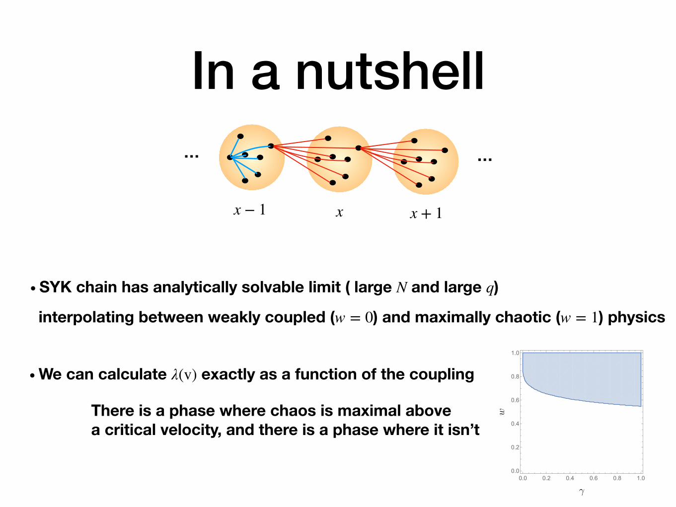
In a nutshell… …

x x + 1x − 1

∙ SYK chain has analytically solvable limit ( large N and large q)

interpolating between weakly coupled (w = 0) and maximally chaotic (w = 1) physics

∙ We can calculate λ(v) exactly as a function of the coupling

There is a phase where chaos is maximal above a critical velocity, and there is a phase where it isn’t

0.0 0.2 0.4 0.6 0.8 1.00.0

0.2

0.4

0.6

0.8

1.0

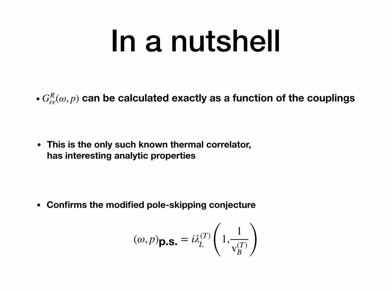
In a nutshell∙ GR

εε(ω, p) can be calculated exactly as a function of the couplings

(ω, p)p.s. = iλ(T)L (1,

1v(T)

B )• Confirms the modified pole-skipping conjecture

• This is the only such known thermal correlator, has interesting analytic properties

Summary