Poisson and Laplace’s Equation - UCSD Mathematicsbdriver/231-02-03/Lecture_Notes/pde9.pdf ·...

126 BRUCE K. DRIVER†

9. Poisson and Laplace’s Equation

For the majority of this section we will assume Ω ⊂ Rn is a compact manifoldwith C2 — boundary. Let us record a few consequences of the divergence theoremin Proposition 8.28 in this context. If u, v ∈ C2(Ωo) ∩ C1(Ω) and R

Ω

|4u|dx < ∞then

(9.1)ZΩ

4u · vdm = −ZΩ

∇u ·∇vdm+

Z∂Ω

v∂u

∂ndσ

and if furtherRΩ

|4u|+ |4v|dx <∞ then

(9.2)ZΩ

(4uv −4v u)dm =

Z∂Ω

µv∂u

∂n− ∂v

∂nu

¶dσ.

Lemma 9.1. Suppose u ∈ C2(Ωo)∩C1(Ω), ∆u = 0 on Ωo and u = 0 on ∂Ω. Thenu ≡ 0. Similarly if ∆u = 0 on Ωo and ∂nu = 0 on ∂Ω, then u is constant on eachconnected component of Ω.

Proof. Letting v = u in Eq. (9.1) shows in either case that

0 = −ZΩ

∇u ·∇udm+

Z∂Ω

u∂u

∂ndσ = −

ZΩ

|∇u|2 dm.

This then implies ∇u = 0 on Ωo and hence u is constant on the connected compo-nent of Ωo. If u = 0 on ∂Ω, these constants must all be zero.

Proposition 9.2 (Laplacian on radial functions). Suppose f(x) = F (|x|) , then

(9.3) 4f(x) =1

rn−1d

dr(rn−1F 0(r))

¯r=|x|

= F 00(|x|) + (n− 1)|x| F 0(|x|).

In particular ∆F (|x|) = 0 implies ddr (r

n−1F 0(r)) = 0 and hence F 0(r) = Ar1−n.That is to say

F (r) =

½Ar2−n +B if n 6= 2A ln r +B if n = 2.

PDE LECTURE NOTES, MATH 237A-B 127

Proof. Since (∂vf)(x) = F 0(|x|) ∂v|x| = F 0(|x|)x · v where x = x|x| , ∇f(x) =

F 0(|x|)x. Hence for g ∈ C1c (Rn),ZRn4f(x)g(x)dx = −

ZRn∇f(x) ·∇g(x) dx

= −ZRn

F 0(r)x ·∇g(rx) dx

= −ZSn−1×[0,∞)

F 0(r)d

drg(rω) rn−1dr dσ(ω)

=

ZSn−1×[0,∞)

d

dr(rn−1F 0(r))g(rω)dr dσ(ω)

=

ZSn−1×[0,∞)

1

rn−1d

dr(rn−1F 0(r)) g(rω)rn−1 dr dσ(ω)

=

ZRn

1

rn−1d

dr(rn−1F 0(r))

¯r=|x|

g(x) dx.

Since this is valid for all g ∈ C1c (Rn), Eq. (9.3) is valid. Alternatively, we maysimply compute directly as follows:

4f(x) = ∇ · [F 0(|x|)x] = ∇F 0(|x|) · x+ F 0(|x|)∇ · x

= F 00(|x|)x · x+ F 0(|x|)∇ · x

|x| = F 00(|x|) + F 0(|x|)½

n

|x| −x

|x|2 · x¾

= F 00(|x|) + (n− 1)|x| F 0(|x|).

Notation 9.3. For t > 0, let

(9.4) α(t) := αn(t) := cn

½1

tn−2 if n 6= 2ln t if n = 2,

where cn =½ 1

(n−2)σ(Sn−1) if n 6= 2− 12π if n = 2.

Also let

(9.5) φ(y) = φn(y) := α (|y|) = cn

½ 1|y|n−2 if n 6= 2ln |y| if n = 2.

An important feature of α is that

(9.6) α0(t) = cn

½ −(n− 2) 1tn−1 if n 6= 2

1t if n = 2

= − 1

σ(Sn−1)1

tn−1

for all n. This then implies, for all n, that

(9.7) ∇φ(x) = ∇ [α (|x|)] = α0(|x|)x = − 1

σ(Sn−1)1

|x|n−1 x = −1

σ(Sn−1)1

|x|nx.

One more piece of notation will be useful in the sequel.

Notation 9.4 (Averaging operator). Suppose µ is a finite measure on some spaceΩ, we will define Z

−Ω

fdµ :=1

µ(Ω)

ZΩ

fdµ.


For example if Ω is a compact manifold with C2 — boundary in Rn thenZ−Ω

f(x)dx =1

m(Ω)

ZΩ

f(x)dx =1

Vol(Ω)

ZΩ

f(x)dx

and Z−∂Ω

fdσ =1

σ(∂Ω)

Z∂Ω

f(x)dx =1

Area(∂Ω)

Z∂Ω

f(x)dx.

Theorem 9.5. Let Ω be a compact manifold with C2- boundary, u ∈ C2(Ωo) ∩C1(Ω) with

RΩ|∆u(y)| dy <∞. Then for x ∈ Ω

(9.8) u(x) =

Z∂Ω

µφ(x− y)

∂u

∂n(y)− u(y)

∂φ(x− y)

∂ny

¶dσ −

ZΩ

φ(x− y)4u(y)dy.

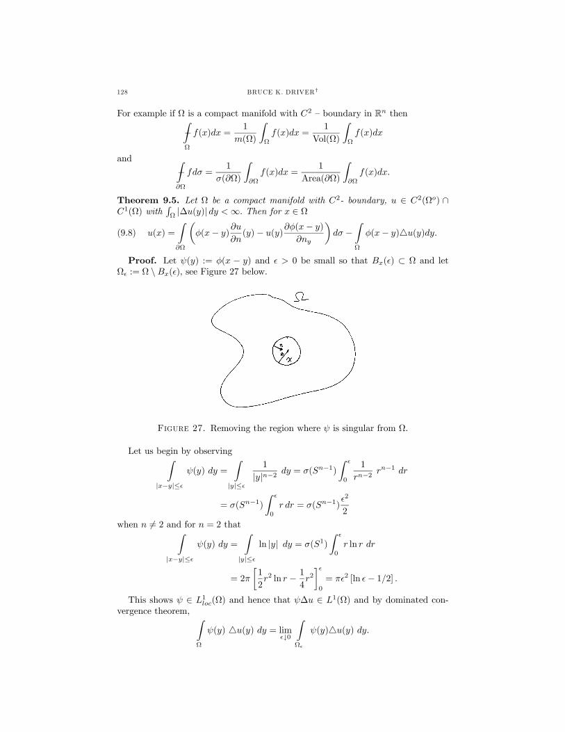
Proof. Let ψ(y) := φ(x − y) and > 0 be small so that Bx( ) ⊂ Ω and letΩ := Ω \Bx( ), see Figure 27 below.

Figure 27. Removing the region where ψ is singular from Ω.

Let us begin by observingZ|x−y|≤

ψ(y) dy =

Z|y|≤

1

|y|n−2 dy = σ(Sn−1)Z0

1

rn−2rn−1 dr

= σ(Sn−1)Z0

r dr = σ(Sn−1)2

2

when n 6= 2 and for n = 2 thatZ|x−y|≤

ψ(y) dy =

Z|y|≤

ln |y| dy = σ(S1)

Z0

r ln r dr

= 2π

·1

2r2 ln r − 1

4r2¸0

= π 2 [ln − 1/2] .

This shows ψ ∈ L1loc(Ω) and hence that ψ∆u ∈ L1(Ω) and by dominated con-vergence theorem, Z

Ω

ψ(y) 4u(y) dy = lim↓0

ZΩ

ψ(y)4u(y) dy.


Using Green’s identity (Eq. (9.2) and Proposition 9.2) and ∆ψ = 0 on Ω , we findZΩ

4u(y)ψ(y) dy =

ZΩ

4ψ(y)u(y) dy +

Z∂Ω

µψ∂u

∂n− ∂ψ

∂nu

¶dσ

=

Z∂Ω

µψ∂u

∂n− ∂ψ

∂nu

¶dσ +

Z∂Ω \∂Ω

µψ∂u

∂n− ∂ψ

∂nu

¶dσ.(9.9)

Working on the last term in Eq. (9.9) we have, for n 6= 2,Z∂B(x, )

ψ(y)∂u

∂n(y) =

Z|y|=

ψ(x+ ω)∂u

∂n(x+ ω)dσ(ω)

=

Z|ω|=1

ψ(x+ ω)∂u

∂n(x+ ω) n−1dσ(ω)

=

Z|ω|=1

1n−2

∂u

∂n(x+ ω) n−1dσ(ω)

=

Z|ω|

∂u

∂n(x+ ω)dσ(ω)→ 0 as ↓ 0.

Similarly when n = 2,Z∂B(x, )

ψ(y)∂u

∂n(y) = ln

Z|ω|=1

∂u

∂n(x+ ω)dσ(ω)→ 0 as ↓ 0.

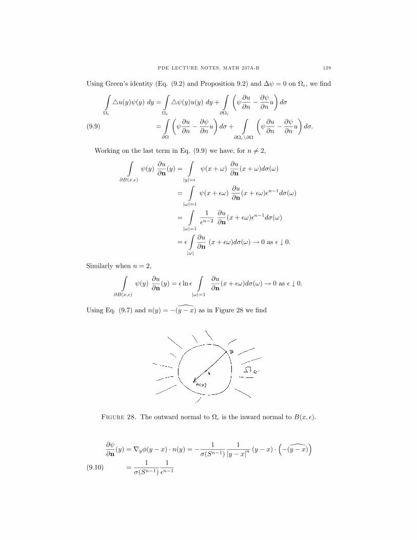
Using Eq. (9.7) and n(y) = −\(y − x) as in Figure 28 we find

Figure 28. The outward normal to Ω is the inward normal to B(x, ).

∂ψ

∂n(y) = ∇yφ(y − x) · n(y) = − 1

σ(Sn−1)1

|y − x|n (y − x) ·³−\(y − x)

´=

1

σ(Sn−1)1n−1(9.10)


and therefore

−Z

∂Ω \∂Ω

u∂ψ

∂ndσ(y) = − 1

σ(Sn−1)1n−1

Z∂B(x, )

u(y)dσ(y)

= −Z−

|ω|=1

u(x+ ω)dσ(ω)→ −u(x) as ↓ 0

by the dominated convergence theorem. So we may pass to the limit in Eq. (9.9)to find Z

Ω

ψ(y) 4u(y)dy =

Z∂Ω

µψ(y)

∂u

∂n− u

∂ψ

∂n

¶dσ(y)− u(x)

which is equivalent to Eq. (9.8).The following Corollary gives an easy but useful extension of Theorem 9.5It will

be us

Corollary 9.6. Keeping the same notation as in Theorem 9.5. Further assumethat h ∈ C2(Ωo) ∩ C1(Ω) and ∆h = 0 and set G(y) := φ(x − y) + h(y). Then westill have the representation formula

(9.11) u(x) =

Z∂Ω

µG(y)

∂u

∂n(y)− u(y)

∂G(y)

∂n

¶dσ −

ZΩ

G(y)4u(y)dy.

Proof. By Green’s identity (Proposition 8.28) with v = h,ZΩ

4u hdm =

ZΩ

(4uh−4h u)dm =

Z∂Ω

µh∂u

∂n− ∂h

∂nu

¶dσ,

i.e.

(9.12) 0 = −ZΩ

4u h dm+

Z∂Ω

µh∂u

∂n− ∂h

∂nu

¶dσ.

Eq. (9.11) now follows by adding Eqs. (9.8) and (9.12).

Corollary 9.7. For all u ∈ C2c (Rn),

(9.13) −ZRn4u(y)φ(y)dy = u(0).

Proof. Let Ω = B(0, R) where R is chosen so large that supp(g) ⊂ Ω, then byTheorem 9.5,

u(0) =

Z∂Ω

µφ(y)

∂u

∂v(y)− u(y)

∂φ(y)

∂vy

¶dσ −

ZΩ

φ(y)4u(y)dy

= −ZΩ

φ(y)4u(y)dy.

Remark 9.8. We summarize (9.13) by saying −4φ = δ.

Formally we expect for reasonable functions ρ that

∆(φ ∗ ρ) = ∆φ ∗ ρ = −δ ∗ ρ = −ρ.


Theorem 9.9. Suppose Ω ⊂o Rn, ρ ∈ C2(Ω) ∩ L1(Ω) and

u(x) :=

ZΩ

φ(x− y)ρ(y)dy = (φ ∗ 1Ωρ) (x),

then−4u = ρ on Ω.

Proof. First assume that ρ ∈ C2c (Ω) in which case we may set ρ := 1Ωρ ∈C2c (Rn). Therefore

u(x) =

ZRn

ρ(y)1

|x− y|n−2 dy =ZRn

ρ(x− y)1

|y|n−2 dy

and so we may differentiate under the integral to find

4u(x) =

ZRn

4xρ(x− y)1

|y|n−2 dy = −ρ(x)

where the last equality follows from Corollary 9.7.For ρ ∈ C2(Ω) ∩ L1(Ω) and x0 ∈ Ω, choose α ∈ C∞c (Ω, [0, 1]) such that α = 1 in

a neighborhood of x0 and let β := 1− α. Then u = (φ ∗ αρ) + (φ ∗ β1Ωρ) and so(9.14) ∆u = ∆ (φ ∗ αρ) +∆ (φ ∗ β1Ωρ) .By what we have just proved

(9.15) ∆ (φ ∗ αρ) (x) = − (αρ) (x) = −ρ(x) for x near x0.Since β = 0 near x0 and

(φ ∗ β1Ωρ) (x) =ZΩ

φ(x− y)β(y)ρ(y)dy,

we may differentiate past the integral to learn

(9.16) ∆ (φ ∗ β1Ωρ) (x) =ZΩ

∆xφ(x− y)β(y)ρ(y)dy = 0

for x near x0. and this completes the proof. The combination of Eqs. (9.14 — 9.16)completes the proof.

9.1. Harmonic and Subharmonic Functions.

Definition 9.10 (HarmonicFunctions). Let Ω ⊂o Rn. A function u ∈ C2(Ω) issaid to be harmonic (subharmonic) on Ω if ∆u = 0 (∆u ≥ 0) on Ω.Because of the Cauchy Riemann equations, the real and imaginary parts of

holomorphic functions are harmonic. For example z2 = (x2 − y2) + 2ixy implies(x2 − y2) and xy are harmonic functions on the plane. Similarly,

ez = ex cos y + iex sin y and

ln(z) = ln r + iθ

impliesex cos y, ex sin y, ln r, and θ(x, y)

are harmonic functions on their domains of definition.


Remark 9.11. If we can choose h in Corollary 9.6 so that G = 0 on ∂Ω, then Eq.(9.11) gives

(9.17) u(x) = −ZΩ

G(y)4u(y)dy −Z∂Ω

u∂G(y)

∂vdσ

which shows how to recover u(x) from ∆u on Ω and u on ∂Ω. The next theorem isa consequence of this remark.

Theorem 9.12 (Mean Value Property). If 4u = 0 on Ω and B(x, r) ⊂ Ω then(9.18) u(x) =

1

σ(∂B(x, r))

Z∂B(x,r)

u(y) dσ(y) =:

Z−

∂B(x,r)

u dσ

More generally if ∆u ≥ 0 on Ω, then(9.19) u(x) ≤

Z−

∂B(x,r)

u dσ

Proof. For y ∈ B(x, r),

G(y) = φ(x− y)− α(r) = α (|x− y|)− α(r)

where α is defined as in Eq. (9.4). Then G(y) = 0 for y ∈ ∂B(x, r) and G(y) > 0for all y ∈ B(x, r) because α is decreasing as is seen from Eq. (9.6). From Eq.(9.10) (using now that n is the outward normal to B(x, r)),

∂G

∂n(x+ rω) = − 1

σ(Sn−1)rn−1for |ω| = 1

and so according to Eq. (9.17) we have

u(x) =1

rn−1σ(Sn−1)

Z∂B(x,r)

udσ −Z

B(x,r)

G(y)4u(y)dy

=

Z−

∂B(x,r)

u dσ −Z

B(x,r)

G(y)4u(y)dy.(9.20)

This completes the proof since G(y) > 0 for all y ∈ B(x, r).

Remark 9.13 (Mean value theorem). Assuming B(x,R) ⊂ Ω and multiplying Eq.(9.18) (Eq. (9.19)) by

σ(∂B(x, r)) = σ(Sn−1)rn−1

and then integrating on 0 ≤ r ≤ R, implies

u(x)m(B(x,R)) = (or ≤)Z R

0

dr

Z∂B(x,r)

u(y) dσ(y)

=

Z R

0

dr rn−1Z

Sn−1

u(x+ rω) dσ(ω) =

ZB(x,R)

udm.

Therefore if ∆u = 0 or ∆u ≥ 0 then(9.21) u(x) =

Z−

B(x,R)

udm or u(x) ≤Z−

B(x,R)

udm respectively


for all B(x,R) ⊂ Ω.Proposition 9.14 (Converse of the mean value property). If u ∈ C(Ω) (or moregenerally measurable and locally bounded) and

(9.22) u(x) =

Z−

∂B(x,r)

u(y)dσ(y)

for all x ∈ Ω and r > 0 such that B(x, r) ⊂ Ω, then u ∈ C∞(Ω) and 4u = 0.Similarly, if u ∈ C2(Ω) and x ∈ Ω and

(9.23) u(x) ≤Z−

∂B(x,r)

u(y)dσ(y)

for all r sufficiently small, then ∆u(x) ≥ 0.Proof. First assume u ∈ C(Ω) and Eq. (9.22) hold which implies

(9.24) u(x) =

Z−S

u(x+ rω)dσ(ω)

for all x ∈ Ω and r sufficiently small, where S = Sn−1 denotes the unit sphere inRn. Let η ∈ C∞c (Rn, [0,∞)) such that η(0) > 0 and

1 =

ZRn

η(|x|2)dx = σ(S)

Z ∞0

η(r2)rn−1dr

and for > 0 let η (x) = −nη³|x|22

´∈ C∞c (Rn) and u (x) = η ∗ u(x). Then for

any x0 ∈ Ω and > 0 sufficiently small, u is a well defined smooth function nearx0. Moreover for x near x0 we have

u (x) =

ZRn

η (x− y)u(y)dy =

Z ∞0

dr rn−1Z

|ω|=1

η (rω)u(x+ rω)dσ(ω)

=

Z ∞0

drrn−1Z

|ω|=1

−nηµr2

2

¶u(x+ rω)dσ(ω)

= u(x)σ(S)

Z ∞0

dr rn−1 −nηµr2

2

¶= u(x)

which shows u is smooth near x0.Now suppose that u ∈ C2, and u satisfies Eq. (9.23), x ∈ Ω and |r| < with

sufficiently small so that

f(r) :=

Z−

∂B(x,r)

u dσ =

Z−

Sn−1

u(x+ rω)dσ(ω)

is well defined. Clearly f ∈ C2 (− , ) , f is an even function of r so f 0(0) = 0,f(0) = u(x) and f(r) ≥ f(0). From these conditions it follows that f 00(0) ≥ 0 forotherwise we would find from Taylor’s theorem that f(r) < f(0) for 0 < |r| < .


On the other hand

0 ≤ f 00(0) =Z−

Sn−1

¡∂2ωu

¢(x)dσ(ω) =

Z−

Sn−1

(∂i∂ju) (x)ωiωjdσ(ω)

= (∂i∂ju) (x)δij

Z−

Sn−1

ω2i dσ(ω) =1

n∆u(x).(9.25)

wherein we have used the symmetry of dσ on Sn−1 to concludeZ−

Sn−1

ωiωjdσ(ω) = 0 if i 6= j

and Z−

Sn−1

ω2i dσ(ω) =1

n

nXj=1

Z−

Sn−1

ω2jdσ(ω) =1

n

Z−

Sn−1

|ω|2 dσ(ω) = 1

n∀ i.

Alternatively, by the divergence theorem,Z−

Sn−1

ωiωjdσ(ω) =

Z−

Sn−1

ωiej · n(ω)dσ(ω) = 1

σ(Sn−1)

ZB(0,1)

∇ · (xiej) dm

=1

σ(Sn−1)m(B(0, 1))δij =

1

nδij .

This completes the proof since if u satisfies (9.22) then f is constant and it followsfrom Eq. (9.25) that ∆u(x) = 0.Second proof of the last statement. Now that we know u is C2 we have by

Eq. (9.20) that ZB(x,r)

G(y)4u(y)dy =

Z−

∂B(x,r)

u dσ − u(x) ≥ 0

and since with α as in Eq. (9.4),ZB(x,r)

G(y)4u(y)dy =

ZB(0,r)

G(x+ y)4u(x+ y)dy

=

Z r

0

ρn−1dρZSn

dωG(x+ ρω)4u(x+ ρω)

=

Z r

0

ρn−1dρ (α(ρ)− α(r))

ZSn

dω4u(x+ ρω)

∼= ∆u(x)σ(Sn−1)Z r

0

ρn−1dρ (α(ρ)− α(r))

= ∆u(x)σ(Sn−1)cn

½r2

2− rn

nrn−2

¾= bnr

2∆u(x)

where bn is a positive constant. From this it follows that ∆u(x) ≥ 0.Third proof of the last statement. If u ∈ C2(Ω) satisfies expand u(x+ rω)

in a Taylor series

u(x+ rω) = u(x) + r∇u(x) · ω + r2

2∂2ωu(x) + o(r3),


and integrate on ω to findZ−

∂B(x,r)

udσ =

Z−

Sn−1

u(x+ rω)dσ(ω)

=

Z−

Sn−1

·u(x) + r∇u(x) · ω + r2

1

2∂2ωu(x) + . . .

¸dσ(ω)

= u(x) +1

2r2∆u(x) + o(r2).

Thus if u satisfies Eq. (9.22) Eq. (9.23) we conclude

u(x) = u(x) +1

2r2∆u(x) + o(r2) or

u(x) ≤ u(x) +1

2r2∆u(x) + o(r2)

from which we conclude ∆u(x) = 0 or ∆u(x) ≥ 0 respectively.Fourth proof of the statement: If u satisfies Eq. (9.22) then ∆u = 0. Since

we already know u is smooth, it is permissible to differentiate Eq. (9.24) in r tolearn,

0 =

Z−

Sn−1

∇u(x+ rω) · ω dσ(ω) =

Z−

Sn−1

∂u

∂n(x+ rω) dσ(ω)

=1

σ(Sn−1)rn−1

Z∂B(x,r)

∇u · n dσ =1

σ(Sn−1)rn−1

ZB(x,r)

4u dm.

Dividing this equation by r and letting r ↓ 0 shows ∆u(x) = 0.Corollary 9.15 (Smoothness of Harmonic Functions). If u ∈ C2(Ω) and 4u =0 then u ∈ C∞(Ω). (Soon we will show u is real analytic, see Theorem 9.16 ofCorollary 9.32 below.)

Theorem 9.16 (Bounds on Harmonic functions). Suppose u is a Harmonic func-tion on Ω ⊂ Rn, x0 ∈ Ω, α is a multi-index with k := |α| and 0 < r < dist(xo, ∂Ω).Then

(9.26) |Dαu(x0)| ≤ Ck

rn+kkukL1(B(x0,r)) ≤

Ck

dist(xo, ∂Ω)n+kkukL1(Ω)

where Ck =(2n+1n k)k

α(n) . In particular one shows that u is real analytic in Ω.

Proof. Let η (x) be constructed as in the proof of Proposition 9.14 so thatu(x) = u ∗ η (x). Therefore, Dαu(x) = u∗Dαη (x) and hence

|Dαu(x0)| ≤ kukL1(B(x0, ))kDαη kL∞ .Now

Dαη (x) = −n 1|α| (D

αη)(x)

so that

|Dαη (x)| = −n 1|α|

¯(Dαη)(

x)¯≤ Cα

1|α|+n

∼= Cα1

r|α|+n


where the last identity is gotten by taking comparable to r. Putting this alltogether then implies that

|Dαu(x0)| ≤ 1

rn+|α|kDαηkL∞kukL1(B(x0,r))

which is an inequality of the form in Eq. (9.26). To get the desired constant wewill have to work harder. This is done in Theorem 7. on p. 29 of the book. Theidea is to use Dαu is harmonic for all α and therefore,

Dαu(x0) =

Z−

B(x0,ρ)

Dαudm =

Z−

B(x0,ρ)

∂iDβudm =

n

σ(Sn−1)ρn

ZB(x0,ρ)

∂iDβudm

=n

σ(Sn−1)ρn

Z∂B(x0,ρ)

Dβunidσ

so that|Dαu(x0)| ≤ n

ρ

°°Dβu°°L∞(B(x0,ρ))

and for α = 0 and x ∈ B(x0, r/2) we have

|u(x)| ≤Z−

B(x,r/2)

|u| dm ≤ 1

|B(0, 1)|µ2

r

¶nkukL1(B(x0,r) .

Using this and similar inequalities along with a tricky induction argument one getsthe desired constants. The details are in Theorem 7. p. 29 and Theorem 10 p.31of the book. (See also Corollary 9.32 below for another proof of analyticity of u.)

Corollary 9.17 (Liouville’s Theorem). Suppose u ∈ C2 (Rn) , ∆u = 0 on Rn and|u(x)| ≤ C(1 + |x|N ) for all x ∈ Rn. Then u is a polynomial of degree at most N.

Proof. We have seen there are constants C|α| <∞ such that

|Dαu(x0)| ≤ C|α|kukL1(B(x0,r))1

rn+|α|

≤ eC|α|rnkukL∞(B(x0,r)) · 1

rn+|α|

∼= C(1 + rN )

r|α|→ 0 as r →∞

when if |α| > N. Therefore Dαu := 0 for all |α| > N and the the result follows byTaylor’s Theorem with remainder,

u(x) =X|α|≤N

Dαu(x0)(x− x0)α

α!.

Corollary 9.18 (Compactness of Harmonic Functions). Suppose Ω ⊂o Rn andun ∈ C2(Ω) is a sequence of harmonic functions such that for each compact setK ⊂ Ω,

CK := sup

½ZK

|un| dm : n ∈ N¾<∞.

Then there is a subsequence vn ⊂ un which converges, along with all of itsderivatives, uniformly on compact subsets of Ω to a harmonic function u.


Proof. An application of Theorem 9.16 shows that for each compact set K ⊂ Ω,supn |∇un|L∞(K) <∞ and hence by the locally compact form of the Arzela-Ascollitheorem, there is a subsequence vn ⊂ un which converges uniformly on compactsubsets of Ω to a continuous function u ∈ C(Ω). Passing to the limit in the meanvalue theorem for harmonic functions along with the converse to the mean valuetheorem, Proposition 9.14, shows u is harmonic on Ω. Since vm → u uniformly oncompacts it follows for any K @@ Ω that

RK|u− vn| dm→ 0. Another application

of Theorem 9.16 then shows Dαvn → Dαu uniformly on compacts.In light of Proposition 9.14, we will extend the notion of subharmonicity as

follows.

Definition 9.19 (Subharmonic Functions). A function u ∈ C(Ω) is said to besubharmonic if for all x ∈ Ω and all r > 0 sufficiently small,

u(x) ≤Z−

∂B(x,r)

u dσ.

The reason for the name subharmonic should become apparent from Corollary 9.25below.

Remark 9.20. Suppose that u, v ∈ C(Ω) are subharmonic functions then so is u+v.Indeed,

u(x) + v(x) ≤Z−

∂B(x,r)

u dσ +

Z−

∂B(x,r)

v dσ =

Z−

∂B(x,r)

(u+ v) dσ.

Theorem 9.21 (Harnack’s Inequality). Let V be a precompact open and connectedsubset of Ω. Then there exists C = C(V,Ω) such that

supV

u ≤ C infV

u

for all non-negative sub-harmonic functions, u, on Ω.

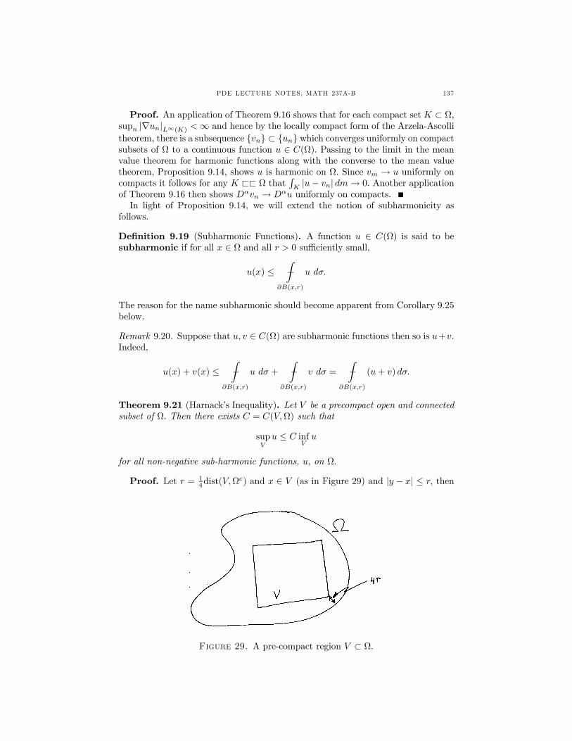
Proof. Let r = 14dist(V,Ω

c) and x ∈ V (as in Figure 29) and |y − x| ≤ r, then

Figure 29. A pre-compact region V ⊂ Ω.


by the mean value inequality in Eq. (9.21) of Remark 9.13,

u(x) =

Z−

B(x,2r)

u(z)dz =1

m(B(0, 1))(2r)n

ZB(x,2r)

u(z)dz

≥ 1

m(B(0, 1))(2r)n

ZB(y,r)

u(z)dz =1

2n

Z−

B(y,r)

u(z)dz =1

2nu(y),

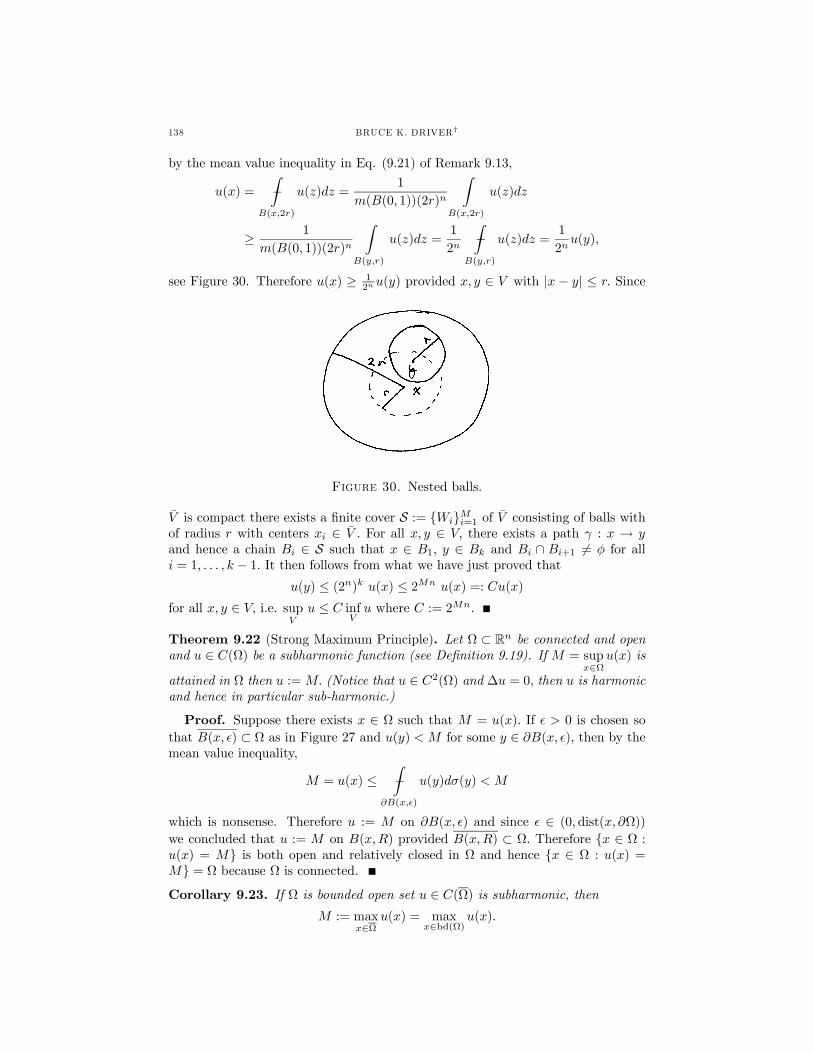
see Figure 30. Therefore u(x) ≥ 12nu(y) provided x, y ∈ V with |x − y| ≤ r. Since

Figure 30. Nested balls.

V is compact there exists a finite cover S := WiMi=1 of V consisting of balls withof radius r with centers xi ∈ V . For all x, y ∈ V, there exists a path γ : x → yand hence a chain Bi ∈ S such that x ∈ B1, y ∈ Bk and Bi ∩ Bi+1 6= φ for alli = 1, . . . , k − 1. It then follows from what we have just proved that

u(y) ≤ (2n)k u(x) ≤ 2Mn u(x) =: Cu(x)

for all x, y ∈ V, i.e. supV

u ≤ C infV

u where C := 2Mn.

Theorem 9.22 (Strong Maximum Principle). Let Ω ⊂ Rn be connected and openand u ∈ C(Ω) be a subharmonic function (see Definition 9.19). If M = sup

x∈Ωu(x) is

attained in Ω then u :=M. (Notice that u ∈ C2(Ω) and ∆u = 0, then u is harmonicand hence in particular sub-harmonic.)

Proof. Suppose there exists x ∈ Ω such that M = u(x). If > 0 is chosen sothat B(x, ) ⊂ Ω as in Figure 27 and u(y) < M for some y ∈ ∂B(x, ), then by themean value inequality,

M = u(x) ≤Z−

∂B(x, )

u(y)dσ(y) < M

which is nonsense. Therefore u := M on ∂B(x, ) and since ∈ (0, dist(x, ∂Ω))we concluded that u := M on B(x,R) provided B(x,R) ⊂ Ω. Therefore x ∈ Ω :u(x) = M is both open and relatively closed in Ω and hence x ∈ Ω : u(x) =M = Ω because Ω is connected.Corollary 9.23. If Ω is bounded open set u ∈ C(Ω) is subharmonic, then

M := maxx∈Ω

u(x) = maxx∈bd(Ω)

u(x).


Again this corollary applies to u ∈ C(Ω) ∩ C2(Ω) such that ∆u = 0.Proof. By Theorem 9.22, if x ∈ Ω is an interior maximum of u, then u =M on

the connected component Ωx of Ω which contains x. By continuity, u is constanton Ωx and in particular u takes on the value M on bd(Ω).

Corollary 9.24. Given g ∈ C(bd(Ω)), f ∈ C(Ω) there exists at most one functionu ∈ C2(Ω) ∩ C(Ω) such that 4u = f on Ω and u = g on bd(Ω).

Proof. If v ∈ C2(Ω) ∩ C(Ω) is another such function then w := u − v ∈C2(Ω) ∩ C(Ω) satisfies ∆w = 0 in Ω and w = 0 on bd(Ω). Therefore applyingCorollary 9.23 to w and −w implies

maxx∈Ω

w(x) = maxx∈bd(Ω)

w(x) = 0 and minx∈Ω

w(x) = minx∈bd(Ω)

w(x) = 0.

Corollary 9.25. Suppose g ∈ C(bd(Ω)) and u ∈ C2(Ω) ∩ C(Ω) such that 4u = 0on Ω. Then w ≤ u for any subharmonic function w ∈ C(Ω) such that w ≤ g onbd(Ω).

Proof. The function −u is subharmonic and so is v = w − u by Remark 9.20.Since v = w − g ≤ 0 on bd(Ω), it follows by Corollary 9.23 that v ≤ 0 on Ω, i.e.w ≤ g on Ω.

9.2. Green’s Functions.

Notation 9.26. Unless otherwise stated, for the rest of this section assume Ω ⊂ Rnis a compact manifold with C2 — boundary.

For x ∈ Ω, suppose there exists h ∈ C2(Ωo) ∩ C1(Ω) which solves(9.27) 4hx = 0 on Ω with hx(y) = φ(x− y) for y ∈ ∂Ω.

Hence if we define

(9.28) G(x, y) = φx(y)− hx(y)

then by the representation formula (Eq. (9.11) also see Remark 9.11) implies

(9.29) u(x) = −ZΩ

G(x, y)4u(y) dy −Z∂Ω

∂G

∂ny(x, y) u(y) dσ(y)

for all u ∈ C2(Ωo) ∩ C1(Ω).Throughout the rest of this subsection we will make the following assumption.

Assumption 2 (Solvability of Dirichlet Problem). We assume that for each g ∈C(∂Ω) there exists h = hg ∈ C2(Ωo) ∩ C1(Ω) such that

∆h = 0 on Ω with h = g on ∂Ω.

In this case we define G(x, y) as in Eq. (9.28). We will (almost) verify that thisassumption holds in Section 9.5 below. The full verification will come later whenwe study Hilbert space methods.

Theorem 9.27. Let G(x, y) be given as in Eq (9.28). Then(1) G(x, y) is smooth on (Ωo × Ωo)\4 where 4 = (x, x) : x ∈ Ωo.(2) G(x, y) = G(y, x) for all x, y ∈ Ω. In particular the function h(x, y) :=

hx(y) is symmetric in x, y and x ∈ Ωo → hx ∈ C(Ω) is a smooth mapping.


(3) If Ω is connected, then G(x, y) > 0 for all (x, y) ∈ (Ωo × Ωo)\4.

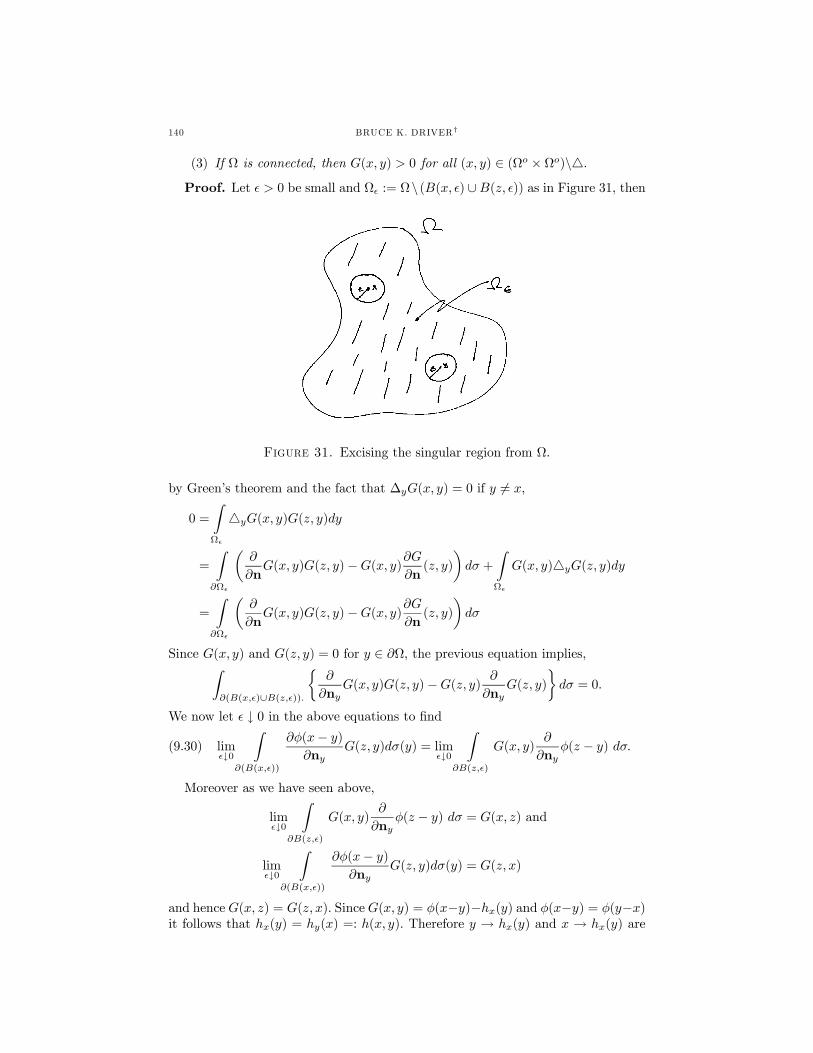
Proof. Let > 0 be small and Ω := Ω\ (B(x, ) ∪B(z, )) as in Figure 31, then

Figure 31. Excising the singular region from Ω.

by Green’s theorem and the fact that ∆yG(x, y) = 0 if y 6= x,

0 =

ZΩ

4yG(x, y)G(z, y)dy

=

Z∂Ω

µ∂

∂nG(x, y)G(z, y)−G(x, y)

∂G

∂n(z, y)

¶dσ +

ZΩ

G(x, y)4yG(z, y)dy

=

Z∂Ω

µ∂

∂nG(x, y)G(z, y)−G(x, y)

∂G

∂n(z, y)

¶dσ

Since G(x, y) and G(z, y) = 0 for y ∈ ∂Ω, the previous equation implies,Z∂(B(x, )∪B(z, )).

½∂

∂nyG(x, y)G(z, y)−G(z, y)

∂

∂nyG(z, y)

¾dσ = 0.

We now let ↓ 0 in the above equations to find

(9.30) lim↓0

Z∂(B(x, ))

∂φ(x− y)

∂nyG(z, y)dσ(y) = lim

↓0

Z∂B(z, )

G(x, y)∂

∂nyφ(z − y) dσ.

Moreover as we have seen above,

lim↓0

Z∂B(z, )

G(x, y)∂

∂nyφ(z − y) dσ = G(x, z) and

lim↓0

Z∂(B(x, ))

∂φ(x− y)

∂nyG(z, y)dσ(y) = G(z, x)

and hence G(x, z) = G(z, x). SinceG(x, y) = φ(x−y)−hx(y) and φ(x−y) = φ(y−x)it follows that hx(y) = hy(x) =: h(x, y). Therefore y → hx(y) and x → hx(y) are


smooth functions. Now by the maximum principle:

|hx(y)− hz(y)| ≤ maxy∈∂Ω

|hx(y)− hz(y)| = maxy∈∂Ω

|φ(x− y)− φ(z − y)|→ 0 as x→ z.

Therefore the map x ∈ Ω → hx ∈ C(Ω) is continuous and in particular the map(x, y)→ h(x, y) is jointly continuous. Finally letting η be as in the proof of Propo-sition 9.14, we find

h(x, y) =

ZΩ

h(ex, y)η(x− ex)dex=

ZΩ×Ω

h(ex, ey) η(y − ey) η(x− ex) dex deyfrom which it follows that in fact h is smooth on Ω× Ω.It only remains to show x → hx ∈ C(Ω) is smooth as well. Fix x ∈ Ω and for

v ∈ Rn, let Hv ∈ C2(Ωo) ∩ C1(Ω) denote the solution to∆Hv = 0 on Ω with Hv(y) = v ·∇φ(x− y) for y ∈ ∂Ω.

Notice that v → Hv is linear and by the maximum principle,

khx+v − hx −HvkL∞(Ω) ≤ khx+v − hx −HvkL∞(∂Ω)= kφ(x+ v − ·)− φ(x− ·)− v ·∇φ(x− ·)kL∞(∂Ω) .

Now,

φ(x+ v − y)− φ(x− y)− v ·∇φ(x− y)

=

Z 1

0

[∇φ(x+ tv − y)−∇φ(x− y)] · vdtso that, by the dominated convergence theorem,

||φ(x+ v − ·)− φ(x− ·)− v ·∇φ(x− ·)||L∞(∂Ω)

≤ |v|Z 1

0

k∇φ(x+ tv − ·)−∇φ(x− ·)kL∞(∂Ω) dt = o (|v|) .This proves x→ hx is differentiable and that ∂vhx = Hv. Similarly one shows thatx→ hx has higher derivatives as well.For the last item, let x ∈ Ωo and choose > 0 sufficiently small so that B(x, ) ⊂

Ωo \ y and G(x, z) > 0 for all z ∈ B(x, ). Then the function u(y) := G(x, y) isHarmonic on Ω0 \B(x, ), u ∈ C(Ω \B(x, )), u = 0 on ∂Ω and u > 0 on ∂B(x, ).Hence by the maximum principle, 0 ≤ u on Ω \B(x, ) and since u is not constantwe must also have u > 0 on Ω0 \ B(x, ). Since > 0 was any sufficiently smallnumber, it follows G(x, y) > 0 for all y ∈ Ωo \ x .Corollary 9.28. Keeping the above hypothesis and assuming ρ ∈ C2(Ωo) ∩ L1(Ω)and g ∈ C(∂Ω), then there is (a necessarily unique) solution u ∈ C2(Ωo)∩C(Ω) to(9.31) ∆u = −ρ with u = g on ∂Ω

which is given by Eq. (9.29).

Proof. According to the remarks just before Eq. (9.29), if a solution to Eq.(9.31) exists it must be given by

(9.32) u(x) =

ZΩ

G(x, y)ρ(y) dy −Z∂Ω

∂G

∂ny(x, y) g(y) dσ(y).


From Assumption 2, there exists a solution v ∈ C2(Ω) ∩ C1(Ω) such that ∆v = 0and v = g on ∂Ω. So replacing u by u− v if necessary, it suffices to prove there isa solution u ∈ C2(Ωo) ∩ C(Ω) such that Eq. (9.31) holds with g ≡ 0. To producethis solution, let

u(x) :=

ZΩ

G(x, y)ρ(y) dy =

ZΩ

φ(x− y)ρ(y) dy −H(x)

where

H(x) :=

ZΩ

h(x, y)ρ(y)dy.

Using the result in Theorem 9.27, one easily shows H ∈ C∞(Ωo) ∩ C1(Ω)and∆H = 0. By Theorem 9.9,

∆x

ZΩ

φ(x− y)ρ(y) dy = −ρ(x) for x ∈ Ω

and therefore u ∈ C2(Ω) and ∆u = −ρ.Remark 9.29. Because of the maximum principle, for any x ∈ Ω the map g ∈C(∂Ω) → hg(x) ∈ C(Ω) is a positive linear functional. So by the Riesz represen-tation theorem, there exists a unique positive probability measure σx on ∂Ω suchthat

hg(x) =

Z∂Ω

g(y)dσx(y) for all g ∈ C(∂Ω).

Evidently this measure is given by

dσx(y) = − ∂G

∂ny(x, y)dσ(y)

and in particular − ∂G∂ny

(x, y) ≥ 0 for all x ∈ Ω and y ∈ ∂Ω. It is in fact easy to see

that − ∂G∂ny

(x, y) > 0 for all x ∈ Ω and y ∈ ∂Ω.

9.3. Explicit Green’s Functions and Poisson Kernels. In this section we willuse the method of images to construct explicit formula for the Green’s functionsand Poisson Kernels for the half plane6, Hn = x ∈ Rn : xn ≥ 0and Balls B(0, a).For x = (x0, z) ∈ Rn−1 × (0,∞) = Hn let Rx := (x0,−z). It is simple to verify|x− y| = |Rx− y| for all x ∈ Hn and y ∈ ∂Hn. Form this and the properties of φ,one concluded, for x ∈ Hn, that hx(y) := φ(y − Rx) is Harmonic in y ∈ Hn andhx(y) = φ(x−y) for all y ∈ ∂Hn. These remarks give rise to the following theorem.

Theorem 9.30. For x, y ∈ Hn, let

G(x, y) := φ(y − x)− φ(y −Rx) = φ(y − x)− φ(Ry − x).

Then G is the Greens function for ∆ on Hn and

K(x, y) := −∂G∂n(x, y) =

2xnσ(Sn−1)

1

|x− y|n for x ∈ Hn and y ∈ ∂Hn

6We will do this again later using the Fourier transform.


is the Poisson kernel for Hn. Furthermore if ρ ∈ C2(Hn) ∩ L1(Hn) and f ∈BC

¡∂Hn

¢, then

u(x) =

ZHn

G(x, y)ρ(y)dy +

Z∂Hn

K(x, y)f(y)dσ(y)

solves the equation

∆u = −ρ on Hn with u = f on ∂Hn.

Proof. First notice that

G(y, x) = φ(x− y)− φ(x−Ry) = φ(x− y)− φ(Rx−RRy) = G(x, y)

since φ is a function of |·| . Therefore, if

u(x) =

ZHn

G(x, y)ρ(y)dy =

ZHn

φ(x− y)ρ(y)dy −ZHn

φ(x−Ry)ρ(y)dy,

we have from Theorem 9.9 that

∆u(x) = −ρ(x)−ZHn∆xφ(x−Ry)ρ(y)dy = −ρ(x).

Since G(x, y) = 0 for x ∈ ∂Hn and so u(x) = 0 for x ∈ ∂Hn. It is left to the readerto show u is continuous on Hn.For x ∈ Hn and y ∈ ∂Hn, we find form Eq. (9.7),

K(x, y) := − ∂G

∂ny(x, y) =

∂

∂ynG(x, y)

=∂

∂yn[φ(y − x)− φ(y −Rx)]

= − 1

σ(Sn−1)1

|y − x|n (y − x) · en + 1

σ(Sn−1)1

|y −Rx|n (y −Rx) · en

=1

σ(Sn−1)2xn

|y − x|n .

Claim: For all x ∈ Hn, Z∂Hn

K(x, y)dy = 1.

It is possible to prove this by direct computation, since (writing x = (x0, xn) asabove) Z

∂HnK(x, y)dy =

2

σ(Sn−1)

ZRn−1

xn

(|x0 − y|2 + x2n)n/2

dy

=2

σ(Sn−1)

ZRn−1

1

(|y|2 + 1)n/2dy

=2

σ(Sn−1)σ(Sn−2)

Z ∞0

rn−21

(r2 + 1)n/2

dr

where in the second equality we have made the change of variables y → xny and inthe last we passed to polar coordinates. When n = 2 we findZ ∞

0

rn−21

(r2 + 1)n/2dr =

Z ∞0

1

r2 + 1dr = π/2


and for n = 3 we may let u = r2 to find

Z ∞0

rn−21

(r2 + 1)n/2

dr =

Z ∞0

r1

(r2 + 1)3/2

dr =1

2

Z ∞0

1

(u+ 1)3/2

du = 1.

These results along with

Z ∞0

rn−21

(r2 + 1)n/2dr =

Z ∞0

¡r2 + 1

¢−n/2drn−1

n− 1 =n/2

n− 1Z ∞0

¡r2 + 1

¢−n/2−12r rn−1dr

=n

n− 1Z ∞0

rn1

(r2 + 1)n+22

dr

allows one to computeR∞0

rn−2 1(r2+1)n/2

dr inductively. I will not carry out thedetails of this method here. Rather, it is more instructive to use Corollary 9.6 toprove the claim. In order to do this let u ∈ C∞c (B(0, 1), [0, 1]) such that u(0) = 1,u(x) = U(|x|) and U(r) is decreasing as r decreases. Then by Corollary 9.6, withu(x) = uM (x) := u(x/M),

(9.33) uM (x) =

Z∂Hn

K(x, y)u(y/M)dσ(y)−M−2ZHn

G(x, y) (4u) (y/M)dy.

By the monotone convergence theorem,

limM↑∞

Z∂Hn

K(x, y)u(y/M)dσ(y) =

Z∂Hn

K(x, y)dσ(y)

and therefore passing the limit in Eq. (9.33) gives

1 =

Z∂Hn

K(x, y)dσ(y)− limM↑∞

M−2 ZHn

G(x, y)4u(y/M)dy

.This latter limit is zero, since

M−2ZHn

G(x, y)4u(y/M)dy = cnM−2ZHn

"1

|x− y|n−2 −1

|Rx− y|n−2#(4u) (y/M)dy

= cnM−2Mn

ZHn

"1

|x−My|n−2 −1

|Rx−My|n−2#4u(y)dy

= cn

ZHn

"1

|x/M − y|n−2 −1

|Rx/M − y|n−2#4u(y)dy.


This latter expression tends to zero and M → ∞ by the dominated convergenceand this proves the claim. (Alternatively, for y large,

1

|x− y|n−2 −1

|Rx− y|n−2 =1

|y|n−2

1¯x|y| − y

¯n−2 − 1¯R x|y| − y

¯n−2

=1

|y|n−2·µ1 + 2

x

|y| · y + . . .

¶−µ1 + 2

Rx

|y| · y + . . .

¶¸= O(

1

|y|n−1 )

and therefore

M−2ZHn

"1

|x− y|n−2 −1

|Rx− y|n−2#(4u) (y/M)dy = O

µM−2

1

Mn−1Mn

¶= O (1/M)→ 0

as M →∞.Since G(x, y) is harmonic in x, it follows that K(x, y) = − ∂

∂nyK(x, y) is still

Harmonic in x. and therefore

u(x) :=

Z∂Hn

K(x, y)f(y)dσ(y) =2

σ(Sn−1)

Z∂Hn

xn|x− y|n f(y)dσ(y)

is harmonic as well. Since

u(x) =2

σ(Sn−1)

Z∂Hn

xn

(|x0 − y|2 + x2n)n/2

f(y)dy

=2

σ(Sn−1)1

xn−1n

Z∂Hn

1³|x0−yxn

|2 + 1´n/2 f(y)dy

it follows from Theorem 7.13 that u((x0, xn))→ f(x0) as xn ↓ 0 uniformly for x0 incompact subsets of ∂Hn.

9.4. Green’s function for Ball. Let r > 0 be fixed, we will construct the Green’sfunction for the ball B(0, r). The idea for a given x ∈ B(0, r), we should find a mirrorlocation, say ρx and a charge q so that

φ(x− y) = qφ (ρx− y) for all |y| = r.

Assuming for the moment that n ≥ 3 and writing q = β(2−n), this leads to theequations

|x− y|2 = |βρx− βy|2 = β2 |ρx− y|2

or equivalently squaring out both sides and using |y| = r,

|x|2 − 2x · y + r2 = β2¡ρ2 − 2ρx · y + r2

¢.

Choosing y ⊥ x and y = rx leads to the conditions

|x|2 + r2 = β2¡ρ2 + r2

¢and

|x|2 − 2r |x|+ r2 = β2¡ρ2 − 2ρr + r2

¢.


Subtracting these two equations implies −2r |x| = −2ρβ2r or equivalently thatρ = |x|/β2. Putting this into the first equation above then implies

|x|2 + r2 =|x|2β2

+ β2r2

or equivalently that

0 = r2β4 −³|x|2 + r2

´β2 + |x|2 .

By the quadratic formula, this implies

β2 =

³|x|2 + r2

´±r³

|x|2 + r2´2− 4r2 |x|2

2r2

=

³|x|2 + r2

´±r³

|x|2 − r2´2

2r2=

³|x|2 + r2

´±³r2 − |x|2

´2r2

= 1 or|x|2r2

.

Clearly the charge β = 1 will not work so we must take β = |x| /r in which case,ρ = r2/ |x| and hence

qφ (ρx− y) = (|x| /r)(2−n) φµr2

x

|x| − y

¶= φ

µrx− |x|

ry

¶.

Let us now verify that our guess has worked. Let us begin by noting the followingidentities for x, y ∈ Rn,(9.34)

¯rx− r−1 |x| y¯2 = ³r2 − 2x · y + r−2 |x|2 |y|2

´and in particular when |y| = r this implies

|xr − |x|y|2 = ¡r2 − 2x · y + |x|2¢ = |x− y|2so that

(9.35) |x− y| = |xr − |x|y| =¯x

|x|r − |x|y

r

¯.

Now the function

hx(y) = φ

µrx− |x|

ry

¶= φ

µ |x|r

µy − r2

x

|x|2¶¶

is harmonic in y and by Eq. (9.35),

hx(y) = φ³xr − |x| y

r

´= φ (xr − |x| y) = φ(x− y) when |y| = r.

Hence we should define the Green’s function for the ball to be given by

G(x, y) = φ(x− y)− hx(y) = φ(x− y)− φ³xr − |x|y

r

´= φ(x− y)− φ

¡xr − r−1|x| |y| y¢

= φ(x− y)− φ

µ |x|r

µy − r2

x

|x|¶¶

.

From Eq. (9.34), it follows that hx(y) = hy(x) and therefore G(x, y) is againsymmetric under the interchange of x and y.


For y ∈ ∂B(0, r), using Eq. (9.7) we find

−K(x, y) = ∂G

∂ny(x, y) = ∂byG(x, y) = ∇yG(x, y) · y

= ∇y

·φ(x− y)− φ

µ |x|r

µy − r2

x

|x|¶¶¸

· y

= − 1

σ(Sn−1)

1

|y − x|n (y − x)− |x|r

1³|x|r

´n ¯y − r2 x

|x|¯n |x|r

µy − r2

x

|x|¶ · y

= − 1

σ(Sn−1)

1

|y − x|n (y − x)− |x|r

1¯|x|r y − rx

¯n µ |x|r y − rx

¶ · y= − 1

σ(Sn−1)

·1

|y − x|n (y − x)− |x|r

1

|x− y|n (|x|y − rx)

¸· y

= − 1

σ(Sn−1) |y − x|n·(y − x)−

µ |x|2r

y − x

¶¸· y

= − 1

σ(Sn−1) |y − x|n·y − |x|

2

ry

¸· y

= − 1

σ(Sn−1)r |y − x|n£r2 − |x|2¤ .

These computations lead to the following theorem.

Theorem 9.31. For x, y ∈ B(0, r), let

G(x, y) := φ(x− y)− φ³xr − |x|y

r

´and if y ∈ ∂B(0, r), let

K(x, y) := −∂G∂n(x, y) =

r2 − |x|2σ(Sn−1)r

|x− y|−n .

Then ρ ∈ C2(B(0, r)) ∩ L1(B(0, r)) and f ∈ C³∂B(0, r)

´, then

(9.36) u(x) =

ZB(0,r)

G(x, y)ρ(y)dy +

Z∂B(0,r)

K(x, y)f(y)dσ(y)

solves the equation

∆u = −ρ on B(0, r) with u = f on ∂B(0, r).

Proof. The proof is essentially the same as Theorem 9.30 but a bit easier. FromTheorem 9.5 with u = 1 it follows again thatZ

∂B(0,r)

K(x, y)dσ(y) = 1.

As x → x0 ∈ ∂B(0, r), the function K(x, y) becomes peaked for y near x0 andgoes to zero away from x0, it follows by the standard approximate δ — functionarguments that Z

∂B(0,r)

K(x, y)f(y)dσ(y)→ f(x0) as x→ x0.


The rest of the argument is the same as before.

Corollary 9.32. Suppose that u is a harmonic function on Ω, then u is real analyticon Ω.

Proof. The condition of being real analytic is local and invariant under trans-lations as is the notion of being harmonic. Hence we may assume 0 ∈ B(0, r) ⊂ Ωfor some r > 0, in which case we have, for |x| < r and f = u|∂B(0,r), that

u(x) =

Z∂B(0,r)

K(x, y)f(y)dσ(y) =r2 − |x|2σ(Sn−1)r

Z∂B(0,r)

|x− y|−n f(y)dσ(y)

=r2 − |x|2σ(Sn−1)r

Z∂B(0,r)

|x− yr|−n f(y)dσ(y).(9.37)

Now

|x− y|−n = |x− yr|−n = r−n¯y − r−1x

¯−n= r−n

Ã1− 2r−1y · x+ |x|

2

r2

!−n/2=: r−n (1− α(x, y))−n/2

where

α(x, y) := 2r−1y · x− |x|2

r2.

Since

|α(x, y)| ≤ 2r−1 |x|+ |x|2

r2≤ 2α0 + α20 < 1

if |x| ≤ α0r and α0 <√2− 1, we find that |x− y|−n has a convergent power series

expansion,

|x− y|−n = r−n∞X

m=0

amα(x, y)m for |x| ≤ α0r.

Plugging this into Eq. (9.37) shows u(x) has a convergent power series expansionin x for |x| ≤ ¡√2− 1¢ r.9.5. Perron’s Method for solving the Dirichlet Problem. For this sectionlet Ω ⊂o Rn be a bounded open set and f ∈ C (bd(Ω),R) be a given function. Weare going to investigate the solvability of the Dirichlet problem:

(9.38) ∆u = 0 on Ω with u = f on bd(Ω).

Let S(Ω) denote those w ∈ C¡Ω¢such that w is subharmonic on Ω and let Sf (Ω)

denote those w ∈ S(Ω) such that w ≤ f on bd(Ω). As we have seen in Corollary9.25, if there is a solution to u ∈ C2(Ω) ∩ C ¡Ω¢ , then w ≤ u for all w ∈ Sf (Ω).This suggests we try to define

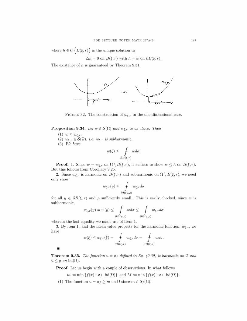
(9.39) u(x) := uf (x) := sup w(x) : w ∈ Sf (Ω) for all x ∈ Ω.Notation 9.33. Given w ∈ S(Ω), ξ ∈ Ω and r > 0 such that B(ξ, r) ⊂ Ω, let (seeFigure 32)

wξ,r(y) =

½w(y) for y ∈ Ω \B(ξ, r)h(y) for y ∈ B(ξ, r)


where h ∈ C³B(ξ, r)

´is the unique solution to

∆h = 0 on B(ξ, r) with h = w on ∂B(ξ, r).

The existence of h is guaranteed by Theorem 9.31.

Figure 32. The construction of wξ,r in the one-dimensional case.

Proposition 9.34. Let w ∈ S(Ω) and wξ,r be as above. Then

(1) w ≤ wξ,r.(2) wξ,r ∈ S(Ω), i.e. wξ,r is subharmonic.(3) We have

w(ξ) ≤Z−

∂B(ξ,r)

wdσ.

Proof. 1. Since w = wξ,r on Ω \ B(ξ, r), it suffices to show w ≤ h on B(ξ, r).But this follows from Corollary 9.25.2. Since wξ,r is harmonic on B(ξ, r) and subharmonic on Ω \ B(ξ, r), we need

only show

wξ,r(y) ≤Z−

∂B(y,ρ)

wξ,rdσ

for all y ∈ ∂B(ξ, r) and ρ sufficiently small. This is easily checked, since w issubharmonic,

wξ,r(y) = w(y) ≤Z−

∂B(y,ρ)

wdσ ≤Z−

∂B(y,ρ)

wξ,rdσ

wherein the last equality we made use of Item 1.3. By item 1. and the mean value property for the harmonic function, wξ,r, we

have

w(ξ) ≤ wξ,r(ξ) =

Z−

∂B(ξ,r)

wξ,rdσ =

Z−

∂B(ξ,r)

wdσ.

Theorem 9.35. The function u = uf defined in Eq. (9.39) is harmonic on Ω andu ≤ g on bd(Ω).

Proof. Let us begin with a couple of observations. In what follows

m := min f(x) : x ∈ bd(Ω) and M := min f(x) : x ∈ bd(Ω) .(1) The function u = uf ≥ m on Ω since m ∈ Sf (Ω).


(2) By the maximum principle w ≤ M on Ω for all w ∈ Sf (Ω) and thereforeuf ≤M on Ω.

(3) If w1, . . . , wm ∈ Sf (Ω), then w = max w1, . . . , wm ∈ Sf (Ω). Indeed forξ ∈ Ω and r small,Z

−∂B(ξ,r)

wdσ ≥Z−

∂B(ξ,r)

widσ ≥ wi(ξ)

for all i.(4) Now suppose ξ ∈ Ω and R > 0 be chosen so that B (ξ,R) ⊂ Ω and D ⊂

B(ξ,R) is a countable set. Then there is a harmonic function wD on B(ξ,R)such that wD = uf on D.

To prove this last item let D := yk∞k=1 and choose wmk ⊂ Sf (Ω) such that

wmk (yk) → u(yk) as m → ∞ for each k. By replacing wm

k by max©w1k, . . . , w

mk

ªif necessary we may assume for each k that wm

k is increasing in m for each k.Letting Wm := max wm

1 , . . . , wmk we find an increasing sequence Wm ⊂ Sf (Ω)

such that Wm(y) ↑ uf (y) for all y ∈ D. Finally define a sequence wm ⊂ Sf (Ω)by wm := (Wm)ξ,2R . By the maximum principle, wm is still increasing and sinceWm ≤ wm and we still have wm(y) ↑ uf (y) for all y ∈ D. We now define wD :=limm→∞wm|B(ξ,R) which exists because wm is increasing and w. We have wD =uf on D and because wm is a bounded and convergent sequence of harmonicfunctions on B(ξ,R), it follows from Corollary 9.18 that w is harmonic on B(ξ,R).This completes the proof of item 4.We now use item 4. to prove uf is continuous at ξ ∈ Ω. To do this let yk∞k=1 ⊂

B (ξ,R) be any sequence such that yk → ξ as k →∞ and let D = ξ∪ yk∞k=1 ⊂B (ξ,R) . Since wD is harmonic and hence continuous,

limk→∞

uf (yk) = limk→∞

wD(yk) = wD(ξ) = uf (ξ)

showing uf is continuous.To show uf is harmonic on B(ξ,R), let D be a countable dense subset of B(ξ,R).

Then the continuity of uf and the fact that uf = wD on D, it follows that uf = wD

on B(ξ,R). In particular uf is harmonic on B(ξ,R). Since ξ is arbitrary, we haveshown uf is harmonic.To complete our program, we want to show that uf extends to a function in

C(Ω) and that uf = f on bd(Ω). For this we will need some assumption on bd(Ω).

Definition 9.36. A function Q ∈ C¡Ω¢is a barrier function for η ∈ bd(Ω) if Q

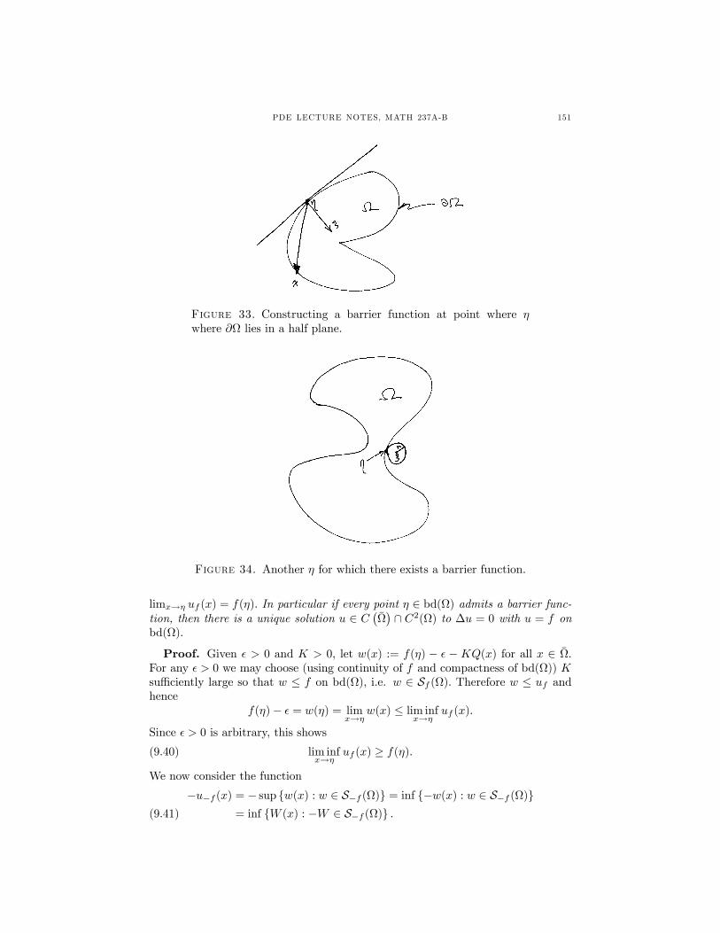
is subharmonic on Ω, Q(η) = 0 and Q(x) < 0 for all x ∈ bd(Ω) \ η .Example 9.37. Suppose that η ∈ bd(Ω) and there exists ξ ∈ Rn such that (x− η)·ξ < 0 for all x ∈ bd(Ω) \ η (see Figure 33 below), then the function Q(x) :=(x− η) · ξ is a barrier function of η.

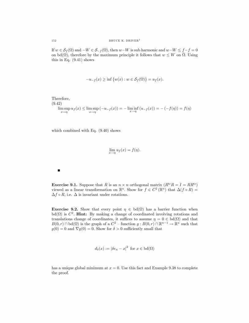
Example 9.38. Suppose that η ∈ bd(Ω) and there exists a ball B(ξ, r)∩ Ω = η(see Figure 34), then Q(x) := α(r)− α(|x− ξ|) is a barrier function for η, where αis defined in Eq. 9.4.

Theorem 9.39. Suppose f ∈ C(bd(Ω)) and u = uf is the harmonic functiondefined by Eq. (9.39) and there exists a barrier function Q for η ∈ bd(Ω). Then


Figure 33. Constructing a barrier function at point where ηwhere ∂Ω lies in a half plane.

Figure 34. Another η for which there exists a barrier function.

limx→η uf (x) = f(η). In particular if every point η ∈ bd(Ω) admits a barrier func-tion, then there is a unique solution u ∈ C

¡Ω¢ ∩ C2(Ω) to ∆u = 0 with u = f on

bd(Ω).

Proof. Given > 0 and K > 0, let w(x) := f(η) − − KQ(x) for all x ∈ Ω.For any > 0 we may choose (using continuity of f and compactness of bd(Ω)) Ksufficiently large so that w ≤ f on bd(Ω), i.e. w ∈ Sf (Ω). Therefore w ≤ uf andhence

f(η)− = w(η) = limx→η

w(x) ≤ lim infx→η

uf (x).

Since > 0 is arbitrary, this shows

(9.40) lim infx→η

uf (x) ≥ f(η).

We now consider the function

−u−f (x) = − sup w(x) : w ∈ S−f (Ω) = inf −w(x) : w ∈ S−f (Ω)= inf W (x) : −W ∈ S−f (Ω) .(9.41)


If w ∈ Sf (Ω) and−W ∈ S−f (Ω), then w−W is sub harmonic and w−W ≤ f−f = 0on bd(Ω), therefore by the maximum principle it follows that w ≤ W on Ω. Usingthis in Eq. (9.41) shows

−u−f (x) ≥ inf w(x) : w ∈ Sf (Ω) = uf (x).

Therefore,(9.42)

lim supx→η

uf (x) ≤ lim supx→η

(−u−f (x)) = − lim infx→η

(u−f (x)) = − (−f(η)) = f(η)

which combined with Eq. (9.40) shows

limx→η

uf (x) = f(η).

Exercise 9.1. Suppose that R is an n× n orthogonal matrix (RtrR = I = RRtr)viewed as a linear transformation on Rn. Show for f ∈ C2 (Rn) that ∆(f R) =∆f R, i.e. ∆ is invariant under rotations.

Exercise 9.2. Show that every point η ∈ bd(Ω) has a barrier function whenbd(Ω) is C2. Hint: By making a change of coordinated involving rotations andtranslations change of coordinates, it suffices to assume η = 0 ∈ bd(Ω) and thatB(0, r) ∩ bd(Ω) is the graph of a C2 — function g : B(0, r) ∩Rn−1 → Rn such thatg(0) = 0 and ∇g(0) = 0. Show for δ > 0 sufficiently small that

dδ(x) := |δen − x|2 for x ∈ bd(Ω)

has a unique global minimum at x = 0. Use this fact and Example 9.38 to completethe proof.


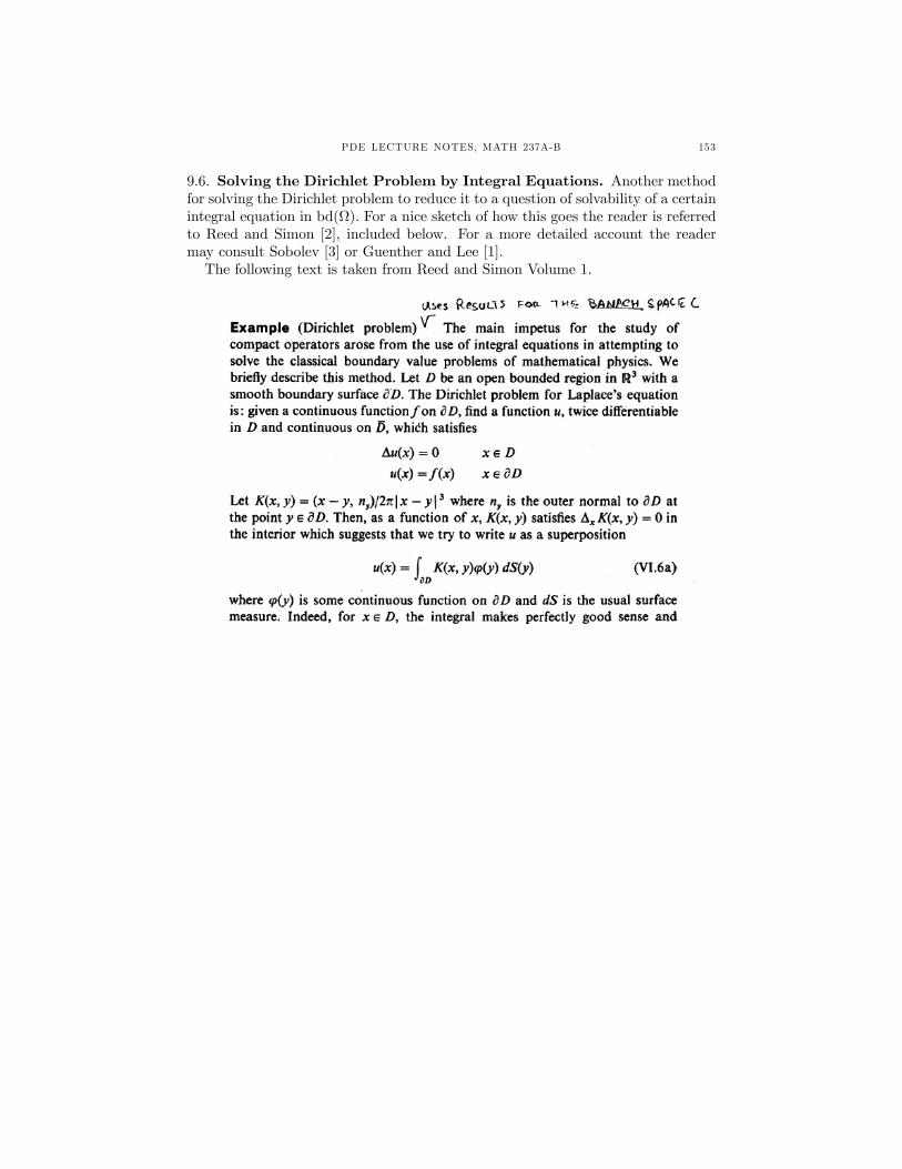
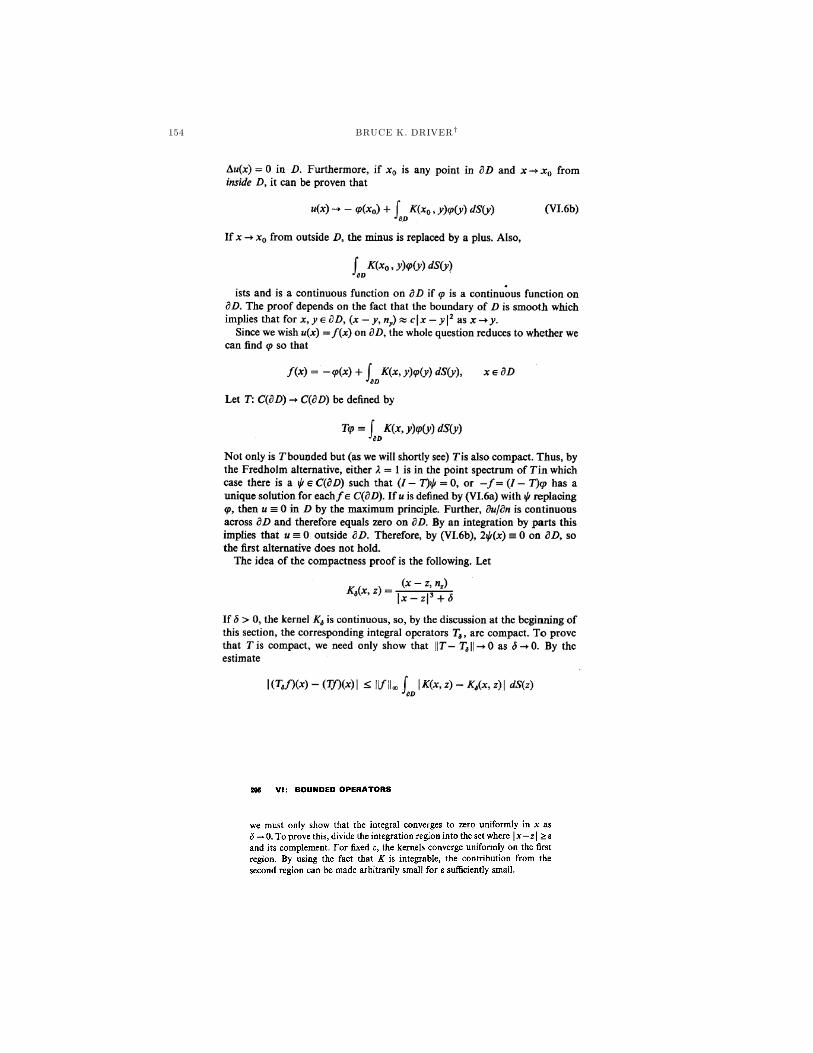
9.6. Solving the Dirichlet Problem by Integral Equations. Another methodfor solving the Dirichlet problem to reduce it to a question of solvability of a certainintegral equation in bd(Ω). For a nice sketch of how this goes the reader is referredto Reed and Simon [2], included below. For a more detailed account the readermay consult Sobolev [3] or Guenther and Lee [1].The following text is taken from Reed and Simon Volume 1.

Poisson and Laplace’s Equation - UCSD Mathematicsbdriver/231-02-03/Lecture_Notes/pde9.pdf ·...

Documents

Transcript of Poisson and Laplace’s Equation - UCSD Mathematicsbdriver/231-02-03/Lecture_Notes/pde9.pdf ·...