Planet Formation Topic: Turbulence Lecture by: C.P. Dullemond.
35
Planet Formation Topic: Turbulence Lecture by: C.P. Dullemond
-
Upload
antonia-dillingham -
Category
Documents
-
view
222 -
download
1
Transcript of Planet Formation Topic: Turbulence Lecture by: C.P. Dullemond.
Planet Formation
Topic:
Turbulence
Lecture by: C.P. Dullemond
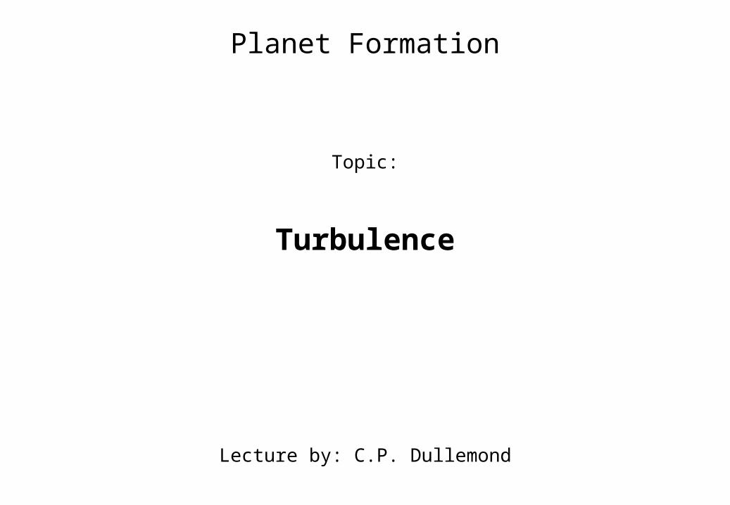
The idea behind the α-formula
Viscosity is length times velocity:
Maximum height of an eddy:
Maximum velicity of an eddy:
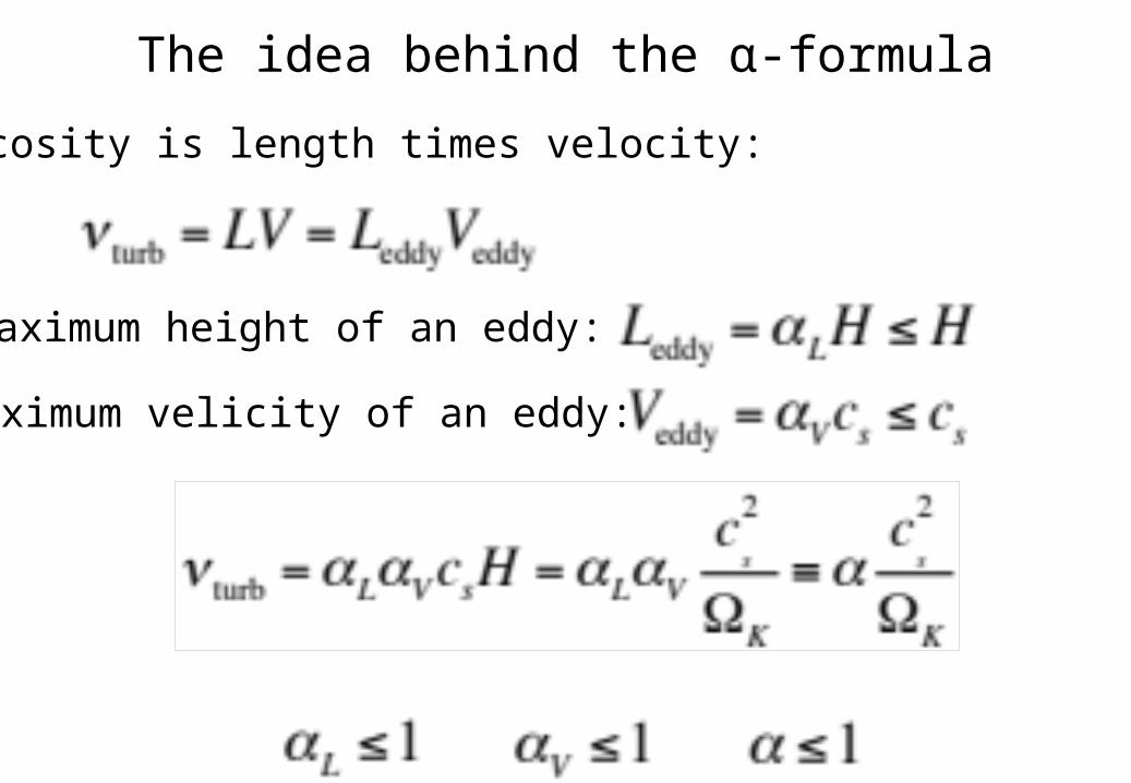
The idea behind the α-formula
Time scales:
Maximum height of an eddy:
Maximum velicity of an eddy:
Simulations show:
Reynolds Number
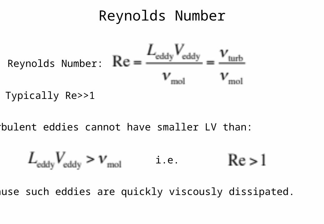
Reynolds Number:
Typically Re>>1
Turbulent eddies cannot have smaller LV than:
i.e.
because such eddies are quickly viscously dissipated.
Kolmogorov Theory ofTurbulence:
The Turbulent Cascade
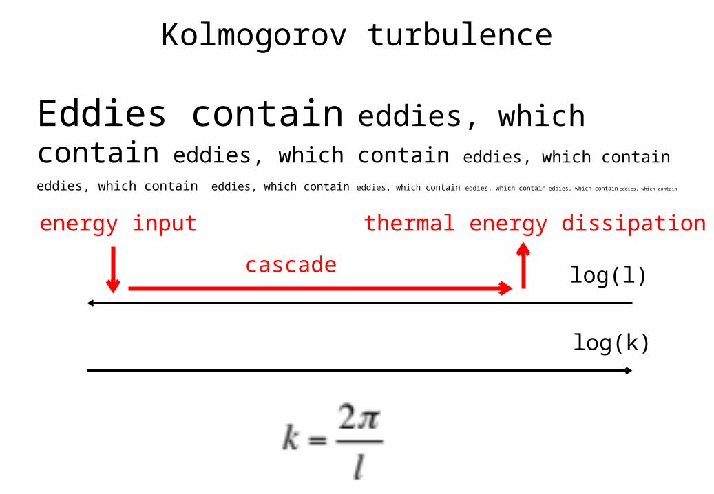
Kolmogorov turbulence
Eddies contain eddies, which contain eddies, which contain eddies, which contain eddies, which contain eddies, which contain eddies, which contain eddies,
which contain eddies, which contain eddies, which contain
log(k)
log(l)
energy input
cascade
thermal energy dissipation

Kolmogorov turbulence
log(E(k))
log(k)
energy input(turbulent driving)
energy dissipation(molecular viscosity)
at the „Kolmogorov scale“
Kolmogorov turbulent cascade(must be a powerlaw!)
Kolmogorov turbulence
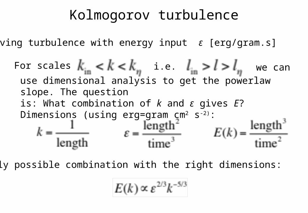
For scales i.e. we can
use dimensional analysis to get the powerlaw slope. The questionis: What combination of k and ε gives E? Dimensions (using erg=gram cm2 s-2):
Driving turbulence with energy input ε [erg/gram.s]
Only possible combination with the right dimensions:
Kolmogorov turbulence
Only possible combination with the right dimensions:
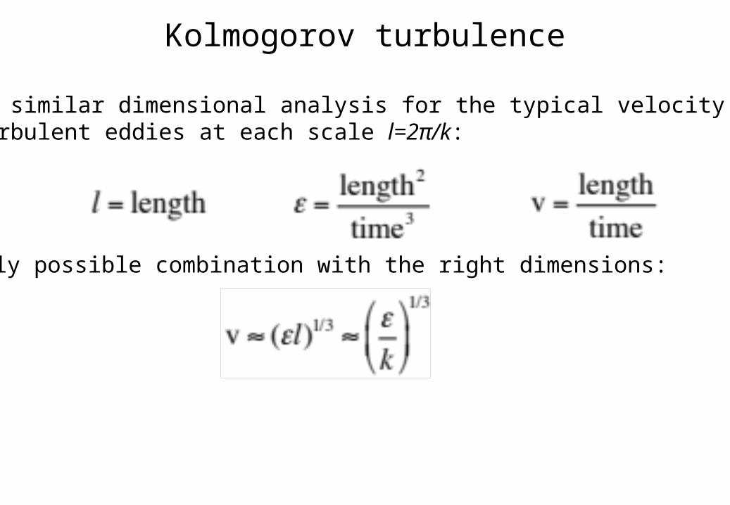
Now a similar dimensional analysis for the typical velocity v of turbulent eddies at each scale l=2π/k:
Kolmogorov turbulence
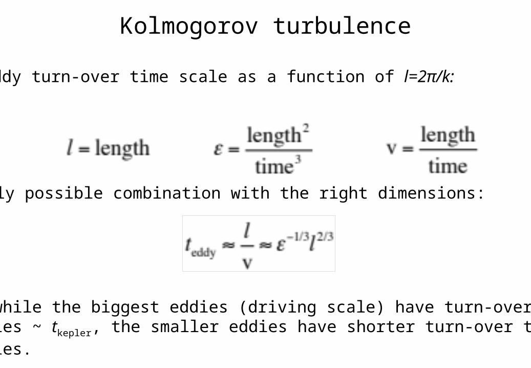
Only possible combination with the right dimensions:
Eddy turn-over time scale as a function of l=2π/k:
So while the biggest eddies (driving scale) have turn-over timescales ~ tkepler, the smaller eddies have shorter turn-over timescales.
Kolmogorov turbulence
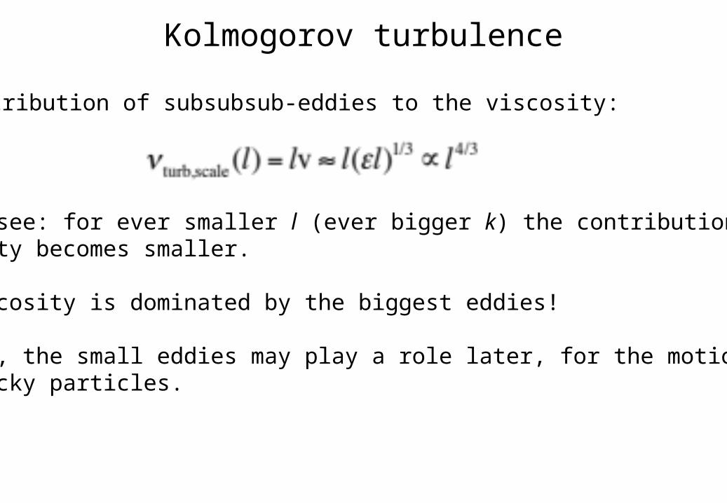
Contribution of subsubsub-eddies to the viscosity:
As you see: for ever smaller l (ever bigger k) the contribution to theviscosity becomes smaller.
The viscosity is dominated by the biggest eddies!
However, the small eddies may play a role later, for the motion ofdust/rocky particles.
Kolmogorov turbulence
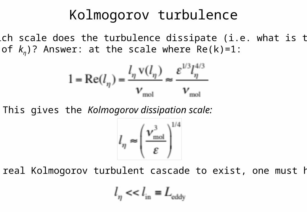
This gives the Kolmogorov dissipation scale:
At which scale does the turbulence dissipate (i.e. what is thevalue of kη)? Answer: at the scale where Re(k)=1:
For a real Kolmogorov turbulent cascade to exist, one must have:

Kolmogorov turbulence
Back to the energy input ε: Let us check if this is consistent withthe viscous heating coefficient Q+ we derived in the previous chapter.
In the cascade region we have (see few slides back):
Let us now make the bold step to assume that this also holds forthe biggest eddies (i.e. that the Kolmogorov powerlaw extentsto the largest eddies):
For Veddy and Leddy we have expressions from α-turbulence theory:
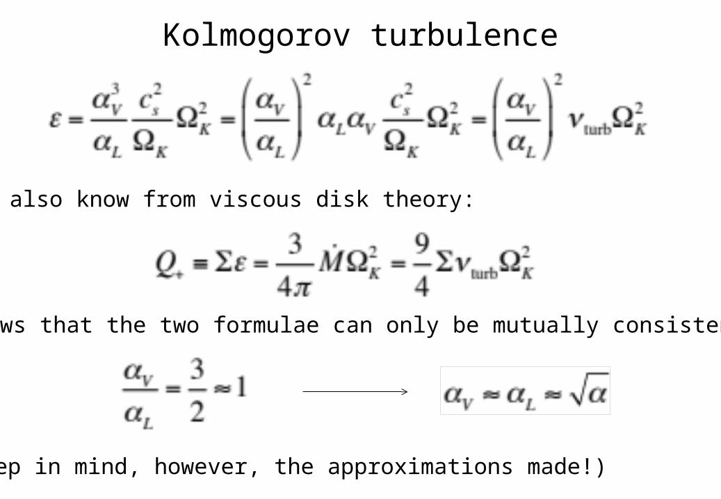
Kolmogorov turbulence
We also know from viscous disk theory:
It follows that the two formulae can only be mutually consistent if:
(keep in mind, however, the approximations made!)
Estimates and numbers
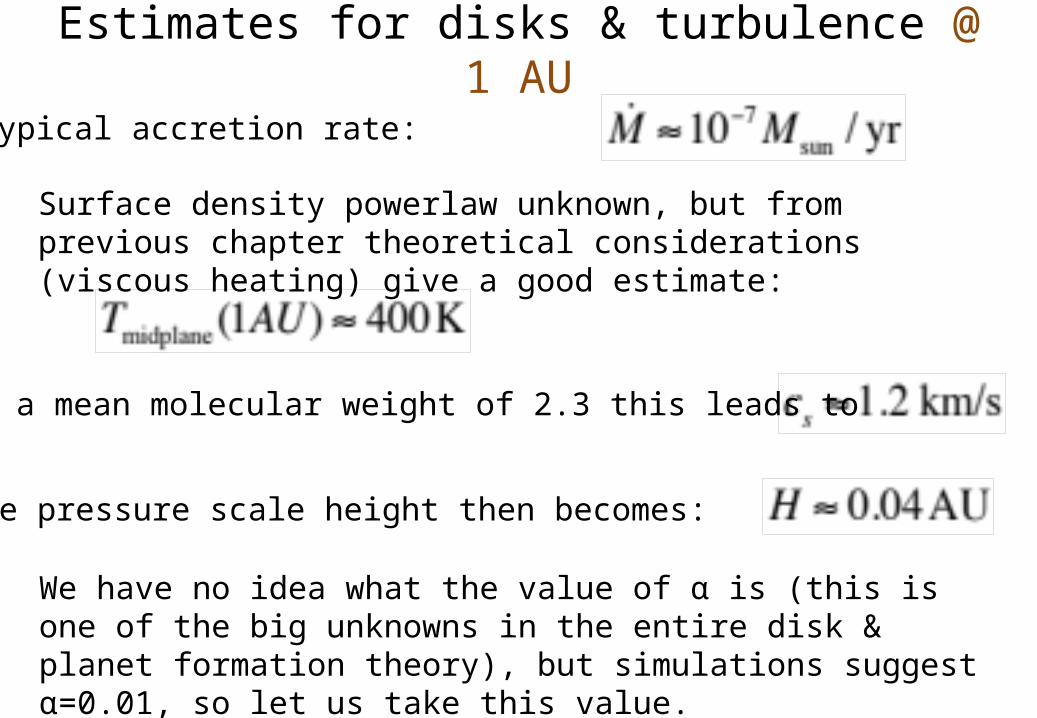
Estimates for disks & turbulence @ 1 AU
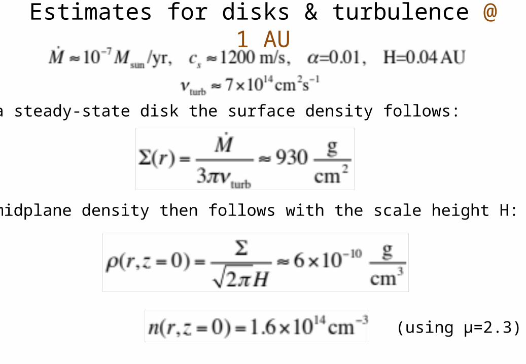
Typical accretion rate:
Surface density powerlaw unknown, but from previous chapter theoretical considerations (viscous heating) give a good estimate:
With a mean molecular weight of 2.3 this leads to
We have no idea what the value of α is (this is one of the big unknowns in the entire disk & planet formation theory), but simulations suggest α=0.01, so let us take this value.
The pressure scale height then becomes:
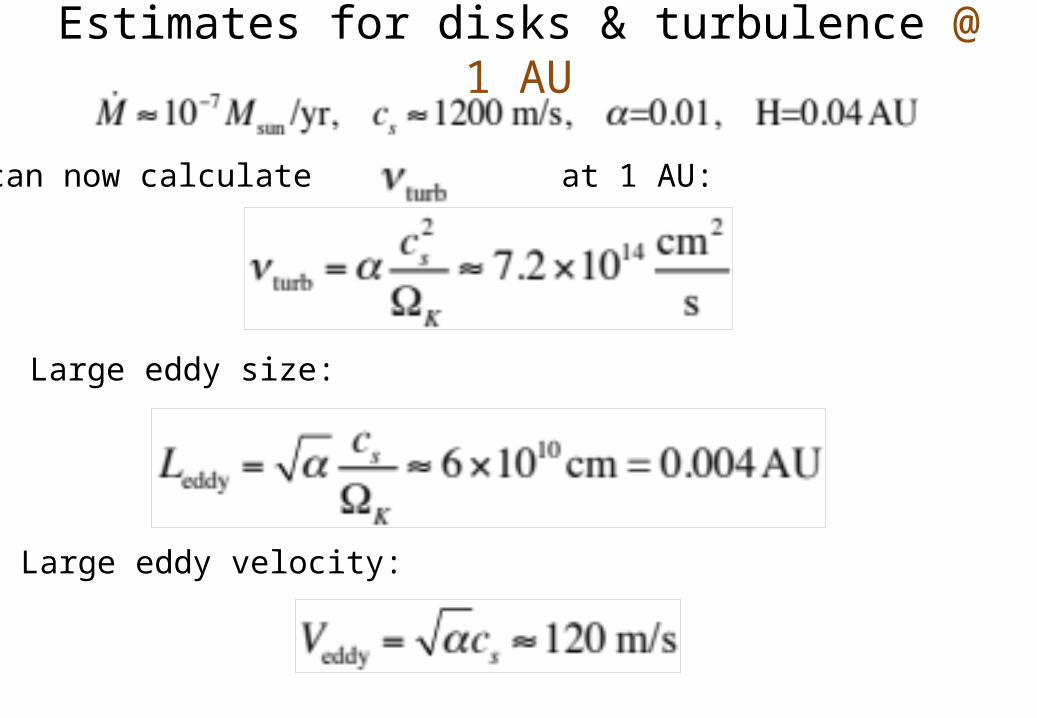
Estimates for disks & turbulence @ 1 AU
We can now calculate at 1 AU:
Large eddy size:
Large eddy velocity:
Estimates for disks & turbulence @ 1 AU
For a steady-state disk the surface density follows:
The midplane density then follows with the scale height H:
(using μ=2.3)
Estimates for disks & turbulence @ 1 AU
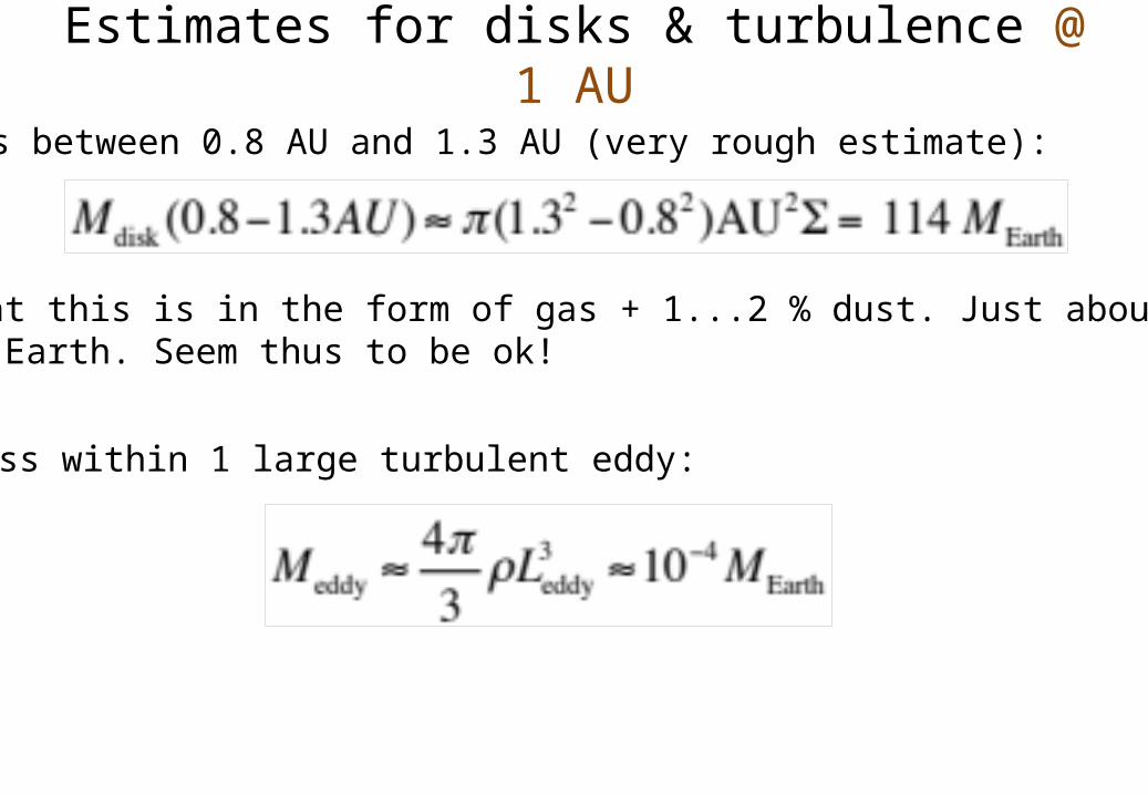
Mass between 0.8 AU and 1.3 AU (very rough estimate):
Note that this is in the form of gas + 1...2 % dust. Just about enough to form Earth. Seem thus to be ok!
Mass within 1 large turbulent eddy:
Estimates for disks & turbulence @ 1 AU
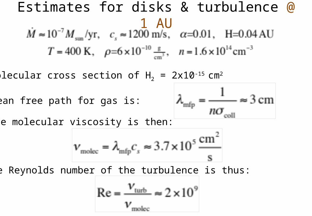
The molecular viscosity is then:
Molecular cross section of H2 = 2x10-15 cm2
Mean free path for gas is:
The Reynolds number of the turbulence is thus:
Estimates for disks & turbulence @ 1 AU
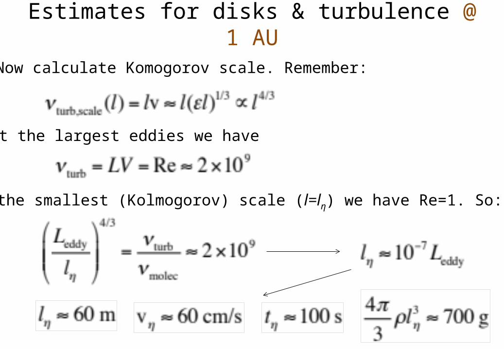
Now calculate Komogorov scale. Remember:
At the largest eddies we have
At the smallest (Kolmogorov) scale (l=lη) we have Re=1. So:
How turbulence is (presumably)driven:
The Magnetorotational Instability
(ref: Book by Phil Armitage)
Magnetorotational Instability
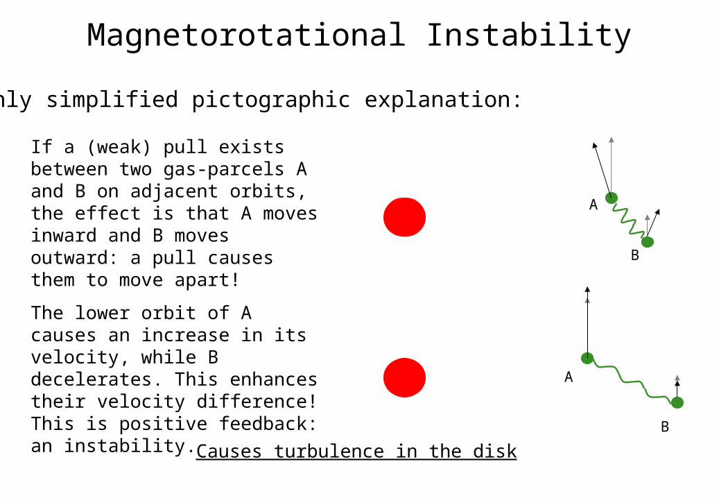
Highly simplified pictographic explanation:
If a (weak) pull exists between two gas-parcels A and B on adjacent orbits, the effect is that A moves inward and B moves outward: a pull causes them to move apart!
A
B
The lower orbit of A causes an increase in its velocity, while B decelerates. This enhances their velocity difference! This is positive feedback: an instability.
A
B
Causes turbulence in the disk
Kelvin-Helmholtz Instability
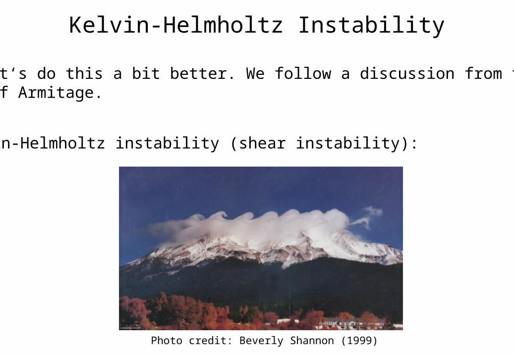
Now let‘s do this a bit better. We follow a discussion from thebook of Armitage.
Kelvin-Helmholtz instability (shear instability):
Photo credit: Beverly Shannon (1999)
Kelvin-Helmholtz Instability
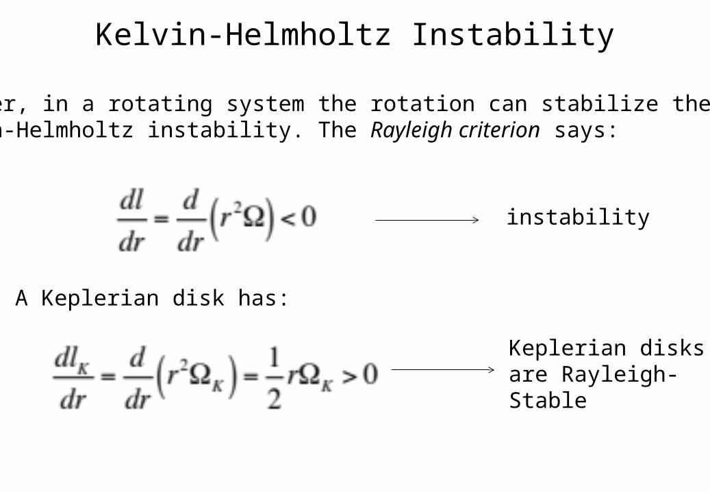
However, in a rotating system the rotation can stabilize the Kelvin-Helmholtz instability. The Rayleigh criterion says:
instability
A Keplerian disk has:
Keplerian disksare Rayleigh-Stable
Magnetorotational Instability
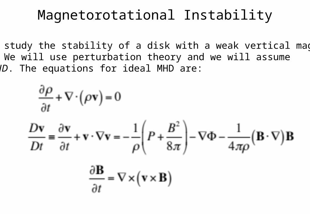
Let us study the stability of a disk with a weak vertical magneticfield. We will use perturbation theory and we will assumeideal MHD. The equations for ideal MHD are:
Magnetorotational Instability
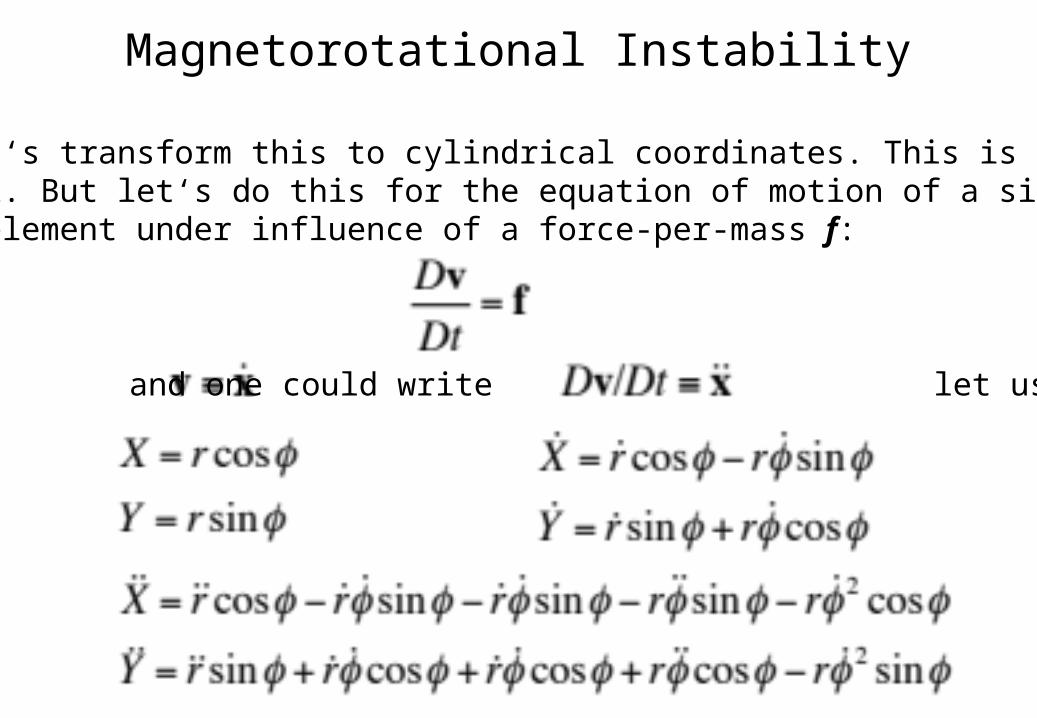
Now let‘s transform this to cylindrical coordinates. This is not trivial. But let‘s do this for the equation of motion of a singlefluid element under influence of a force-per-mass f:
Since and one could write let us write out:
Magnetorotational Instability
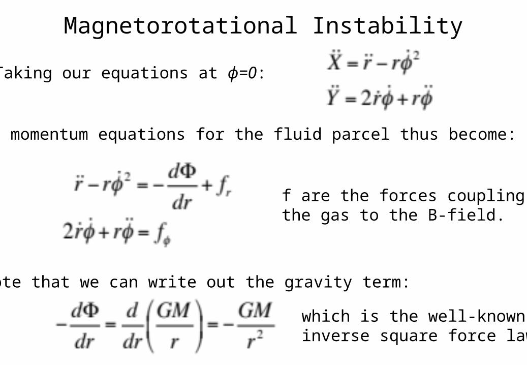
Taking our equations at ϕ=0:
The momentum equations for the fluid parcel thus become:
f are the forces couplingthe gas to the B-field.
Note that we can write out the gravity term:
which is the well-knowninverse square force law
Magnetorotational Instability
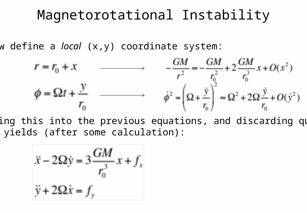
Now define a local (x,y) coordinate system:
Inserting this into the previous equations, and discarding quadraticterms, yields (after some calculation):
Magnetorotational Instability
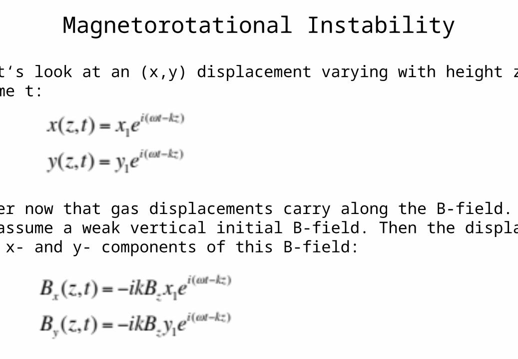
Now let‘s look at an (x,y) displacement varying with height z and time t:
Remember now that gas displacements carry along the B-field.Let‘s assume a weak vertical initial B-field. Then the displacementscreate x- and y- components of this B-field:
Magnetorotational Instability
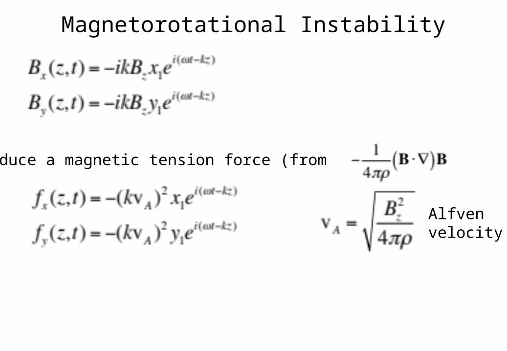
These produce a magnetic tension force (from ):
Alfvenvelocity
Magnetorotational Instability
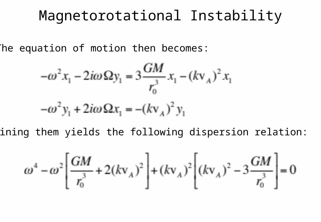
The equation of motion then becomes:
Combining them yields the following dispersion relation:
Magnetorotational Instability
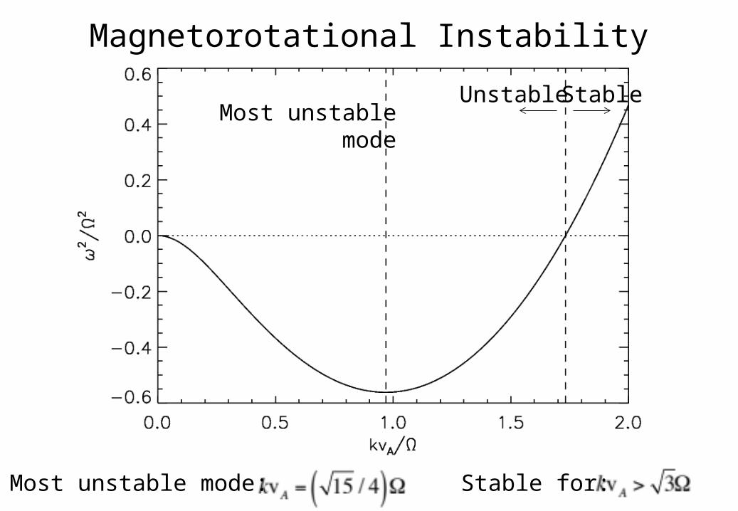
Most unstablemode
StableUnstable
Most unstable mode: Stable for:
Magnetorotational Instability
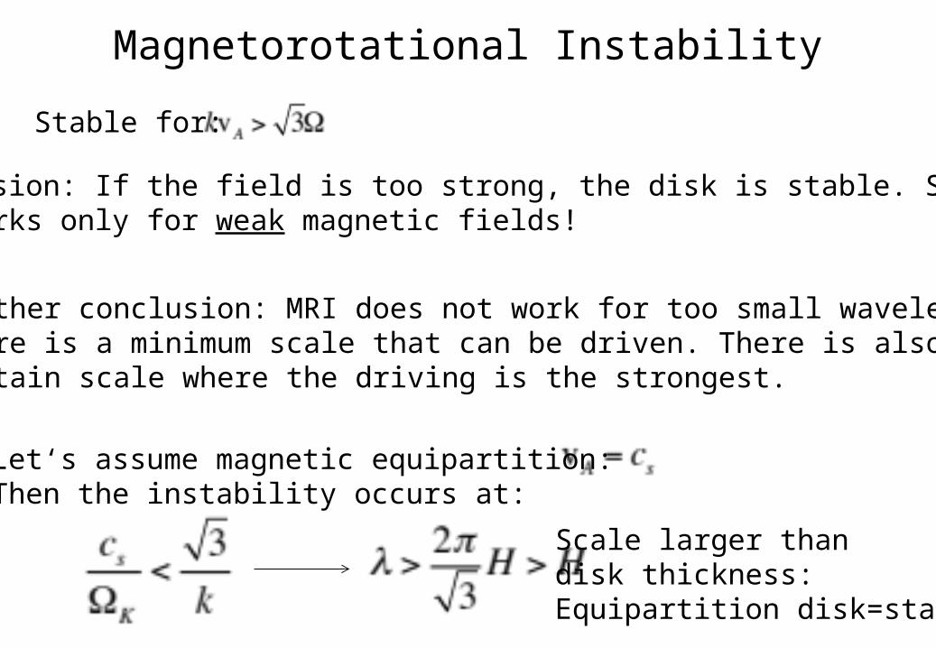
Stable for:
Conclusion: If the field is too strong, the disk is stable. So MRI works only for weak magnetic fields!
Another conclusion: MRI does not work for too small wavelengths.There is a minimum scale that can be driven. There is also a certain scale where the driving is the strongest.
Let‘s assume magnetic equipartition:Then the instability occurs at:
Scale larger thandisk thickness:Equipartition disk=stable
Magnetorotational Instability
Note: This instability works only if the disk is sufficiently ionizedfor ideal MHD equations to be valid.
Only a tiny bit of ionization is required.
But even that can be problematic, since dust grains veryefficiently „vacuum clean“ away free electrons.
This leads to so called „dead zones“ in disks.
The debate for what causes turbulence in disks remains wide opentoday.