plane waves, transmission lines and waveguides - Jenn, David C
84
Naval Postgraduate School Department of Electrical & Computer Engineering Monterey, California EC3630 Radiowave Propagation PLANE WAVES, TRANSMISSION LINES AND WAVEGUIDES by Professor David Jenn t (version 1.3)
Transcript of plane waves, transmission lines and waveguides - Jenn, David C
Naval Postgraduate School Department of Electrical & Computer Engineering Monterey, California
EC3630 Radiowave Propagation
PLANE WAVES, TRANSMISSIONLINES AND WAVEGUIDES
by Professor David Jenn
t
(version 1.3)
1
Naval Postgraduate School Department of Electrical & Computer Engineering Monterey, California
Electromagnetic Fields and Waves (1)
Electrical properties of a medium are specified by its constitutive parameters:
• permeability, µ = µoµr (for free space, µ ≡ µo = 4π ×10−7 H/m)• permittivity, ε = εoεr (for free space, ε ≡ εo = 8.85 ×10⁻¹² F/m)• conductivity, σ (for a metal, σ ~ 107 S/m)
Electric and magnetic field intensities are r E ( x, y, z, t) V/m and
r H (x, y,z, t) A/m
• they are vector functions space and time, e.g., in cartesian coordinates
r E (x,y, z,t) = ˆ x Ex (x,y, z,t) + ˆ y Ey (x,y, z,t) + ˆ z Ez (x,y, z,t)
• similar expressions for other coordinates systems• fields arise from currents
r J and charges ρv on the source (
r J is the volume
current density in A/m2 and ρv is volume charge density in C/m3)
Electromagnetic fields are completely described by Maxwell’s equations:
(1) ∇ ×r E = −µ ∂
r H
∂t(3) ∇⋅
r H = 0
(2) ∇ ×r H =
r J + ε
∂r E
∂t(4) ∇⋅
r E = ρv / ε
2
Naval Postgraduate School Department of Electrical & Computer Engineering Monterey, California
Electromagnetic Fields and Waves (2)
Most sources of electromagnetic fields have a sinusoidal variation in time (time-harmonicsources). All of the field quantities associated with the sources will have the samesinusoidal time variation. Therefore, we suppress the time dependence for convenience,and work with a time independent quantity called a phasor. The two are related by
tjezEtzE ω)(Re),(rr
=
• r E (z) is the phasor representation;
r E (z, t) is the instantaneous quantity
• ⋅Re is the real operator (i.e., “take the real part of”)• 1−=j
Since the time dependence varies as tje ω , the time derivatives in Maxwell’s equationscan be replaced by ∂ / ∂t ≡ jω in the time-harmonic case:
(1) ∇ ×
r E = − jωµ
r H (3) ∇⋅
r H = 0
(2) ∇ ×r H =
r J + jωε
r E (4) ∇⋅
r E = ρv / ε
Any fields or waves that exist in a particular region of space must satisfy Maxwell’sequations and the appropriate boundary conditions.
3
Naval Postgraduate School Department of Electrical & Computer Engineering Monterey, California
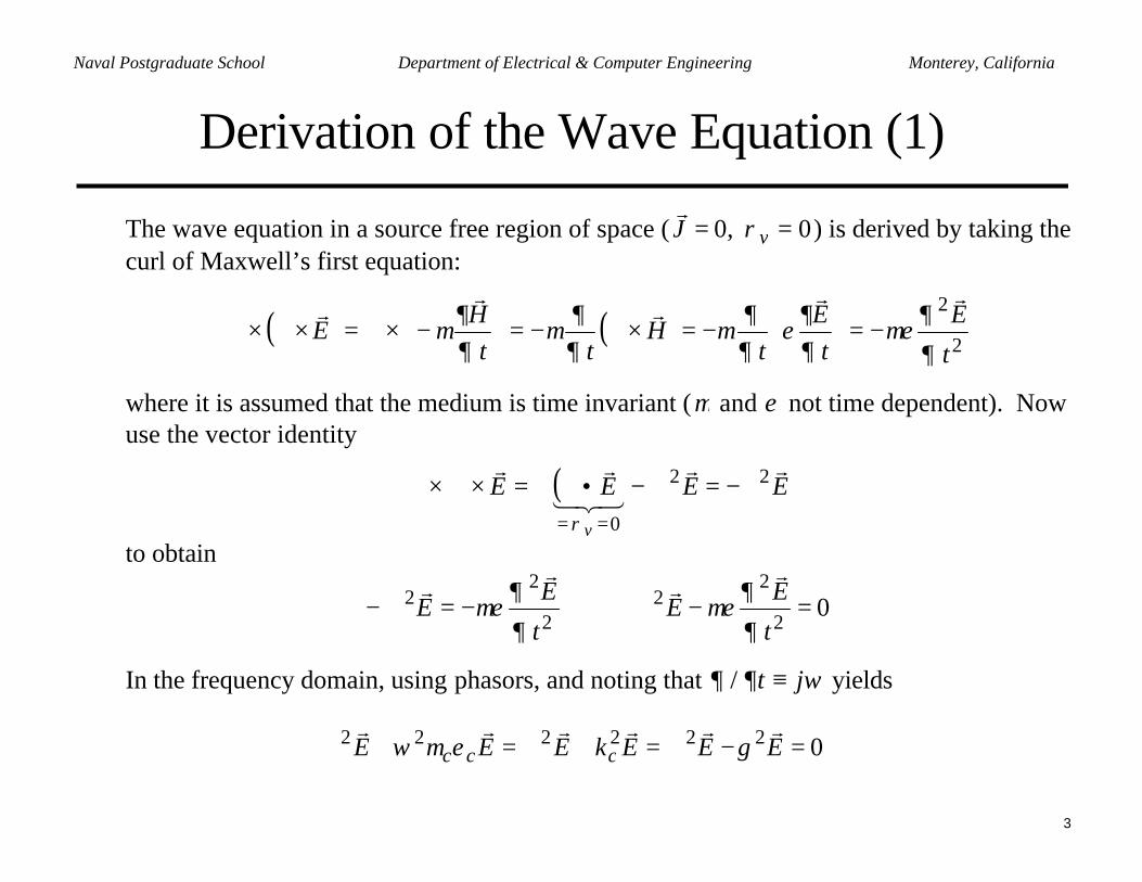
Derivation of the Wave Equation (1)
The wave equation in a source free region of space ( 0,0 == vJ ρr
) is derived by taking thecurl of Maxwell’s first equation:
( ) ( )2
2
t
Et
Et
Htt
HE
∂
∂µε
∂∂
ε∂∂
µ∂∂
µ∂∂
µrrrrr
−=
−=×∇−=
−×∇=×∇×∇
where it is assumed that the medium is time invariant (µ and ε not time dependent). Nowuse the vector identity
( ) EEEE
v
rr321rr 22
0
−∇=∇−•∇∇=×∇×∇== ρ
to obtain
02
22
2
22 =−∇⇒−=∇−
t
EE
t
EE
∂
∂µε
∂
∂µε
rrrr
In the frequency domain, using phasors, and noting that ∂ / ∂t ≡ jω yields
0222222 =−∇=+∇=+∇ EEEkEEE cccrrrrrr
γεµω
4
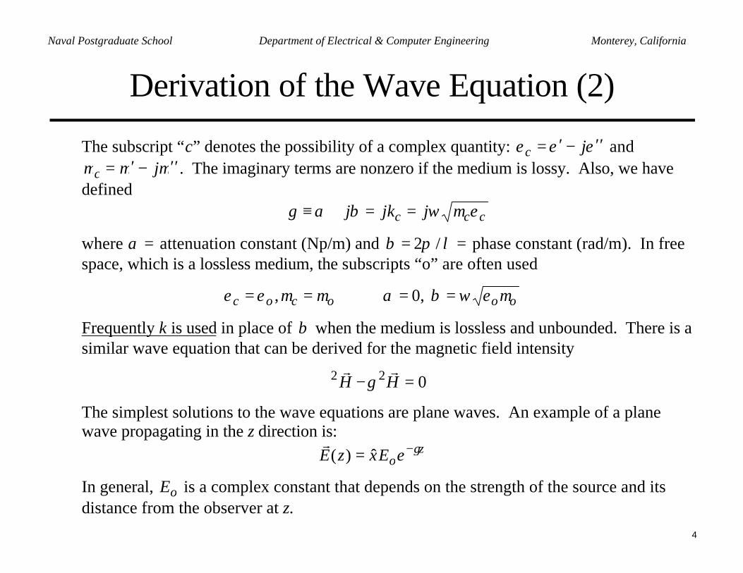
Naval Postgraduate School Department of Electrical & Computer Engineering Monterey, California
Derivation of the Wave Equation (2)
The subscript “c” denotes the possibility of a complex quantity: εεε ′′−′= jc andµµµ ′′−′= jc . The imaginary terms are nonzero if the medium is lossy. Also, we have
defined
ccc jjkj εµωβαγ ==+≡
where α = attenuation constant (Np/m) and == λπβ /2 phase constant (rad/m). In freespace, which is a lossless medium, the subscripts “o” are often used
ooococ µεωβαµµεε ==⇒== ,0,
Frequently k is used in place of β when the medium is lossless and unbounded. There is asimilar wave equation that can be derived for the magnetic field intensity
022 =−∇ HHrr
γ
The simplest solutions to the wave equations are plane waves. An example of a planewave propagating in the z direction is:
zoeExzE γ−= ˆ)(
r
In general, oE is a complex constant that depends on the strength of the source and itsdistance from the observer at z.
5
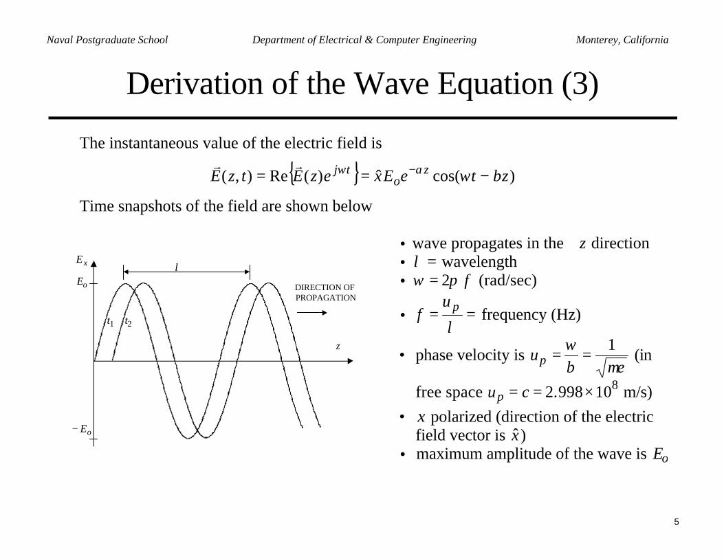
Naval Postgraduate School Department of Electrical & Computer Engineering Monterey, California
Derivation of the Wave Equation (3)
The instantaneous value of the electric field is
)cos(ˆ)(Re),( zteExezEtzE zo
tj βωαω −== −rr
Time snapshots of the field are shown below
z
1t 2t
xE
DIRECTION OF PROPAGATION
oE
oE−
λ
• wave propagates in the + z direction• =λ wavelength• fπω 2= (rad/sec)
• ==λpu
f frequency (Hz)
• phase velocity is εµβ
ω 1==pu (in
free space up = c = 2.998×10⁸ m/s)• x polarized (direction of the electric
field vector is ˆ x )• maximum amplitude of the wave is Eo
6
Naval Postgraduate School Department of Electrical & Computer Engineering Monterey, California
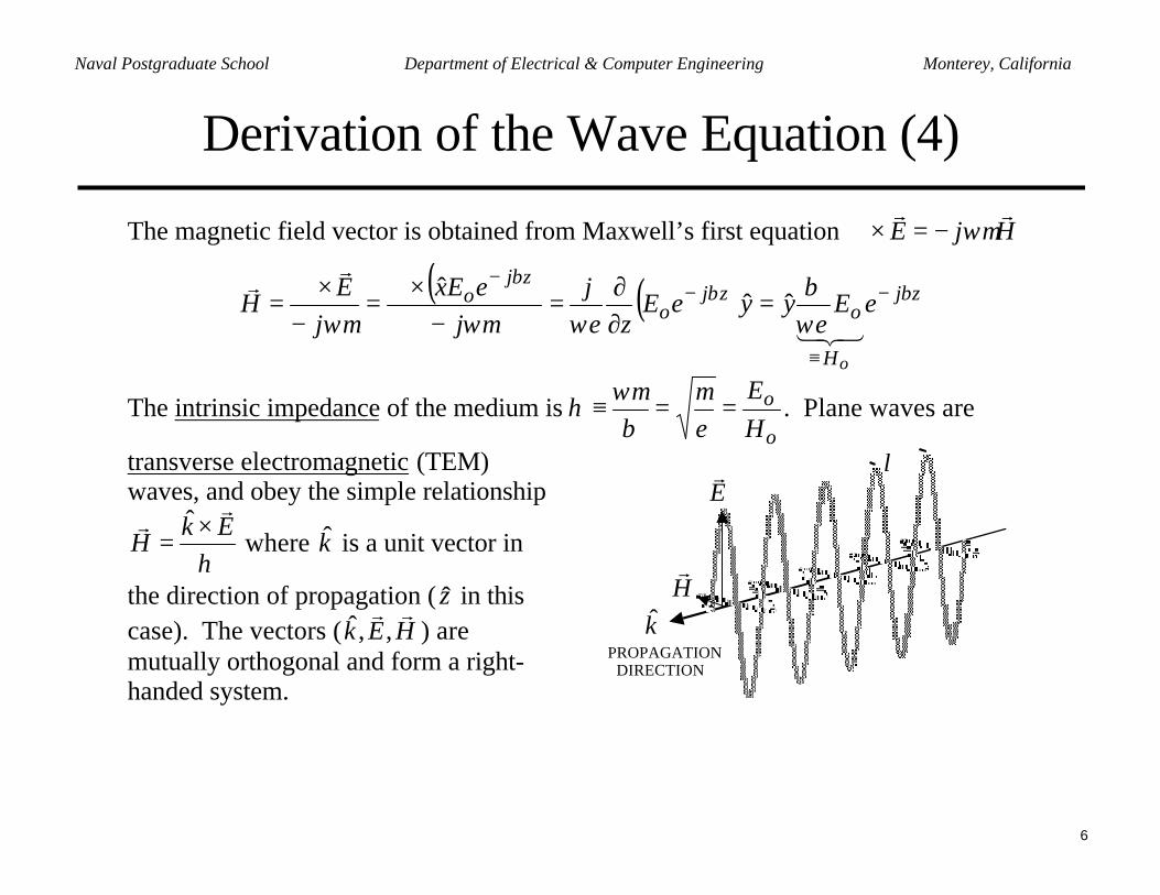
Derivation of the Wave Equation (4)
The magnetic field vector is obtained from Maxwell’s first equation HjErr
ωµ−=×∇
( ) ( ) zj
H
ozj
o
zjo eEyyeE
zj
jeEx
jE
H
o
βββ
ωεβ
ωεωµωµ−
≡
−−
=∂∂
=−
×∇=
−×∇
=321
rrˆˆ
ˆ
The intrinsic impedance of the medium is o
o
HE
==≡εµ
βωµ
η . Plane waves are
transverse electromagnetic (TEM)waves, and obey the simple relationship
ηEk
Hrr ×
=ˆ
where k is a unit vector in
the direction of propagation ( z in thiscase). The vectors ( HEk
rr,,ˆ ) are
mutually orthogonal and form a right-handed system.
PROPAGATION DIRECTION
Hr
Er λ
k
7
Naval Postgraduate School Department of Electrical & Computer Engineering Monterey, California
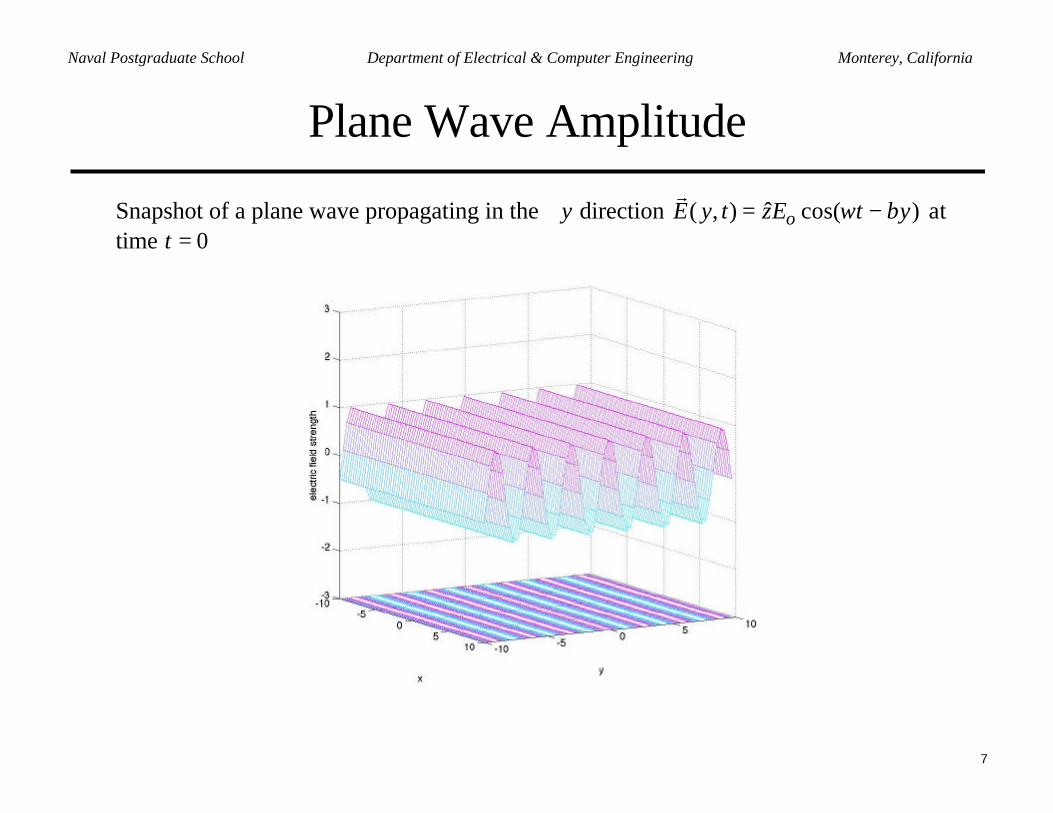
Plane Wave Amplitude
Snapshot of a plane wave propagating in the + y direction )cos(ˆ),( ytEztyE o βω −=r
attime t = 0
8
Naval Postgraduate School Department of Electrical & Computer Engineering Monterey, California
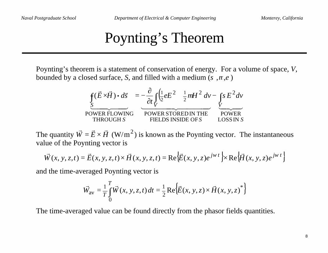
Poynting’s Theorem
Poynting’s theorem is a statement of conservation of energy. For a volume of space, V,bounded by a closed surface, S, and filled with a medium ( εµσ ,, )
( )434214444 34444 214434421
rrr
S
V
S
V
S
S
dvEdvHEt
sdHE
IN LOSSPOWER
2
OF INSIDE FIELDSTHEIN STORED POWER
22
THROUGH FLOWINGPOWER
21
21)( ∫∫∫ −+
∂∂
−=× • σµε
The quantity HEWrrr
×= (W/ 2m ) is known as the Poynting vector. The instantaneousvalue of the Poynting vector is
tjtj ezyxHezyxEtzyxHtzyxEtzyxW ωω ),,(Re),,(Re),,,(),,,(),,,(rrrrr
×=×=
and the time-averaged Poynting vector is
*21
0
1av ),,(),,(Re),,,( zyxHzyxEdttzyxWW
T
T
rrrr×== ∫
The time-averaged value can be found directly from the phasor fields quantities.
9
Naval Postgraduate School Department of Electrical & Computer Engineering Monterey, California
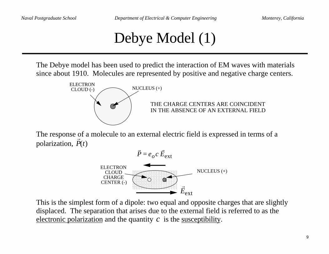
Debye Model (1)
The Debye model has been used to predict the interaction of EM waves with materialssince about 1910. Molecules are represented by positive and negative charge centers.
ELECTRON CLOUD (-) NUCLEUS (+)
THE CHARGE CENTERS ARE COINCIDENT IN THE ABSENCE OF AN EXTERNAL FIELD
The response of a molecule to an external electric field is expressed in terms of apolarization,
r P (t)
ELECTRON CLOUD
CHARGE CENTER (-)
NUCLEUS (+)
extoP Eε χ=r r
extEr
This is the simplest form of a dipole: two equal and opposite charges that are slightlydisplaced. The separation that arises due to the external field is referred to as theelectronic polarization and the quantity χ is the susceptibility.
10
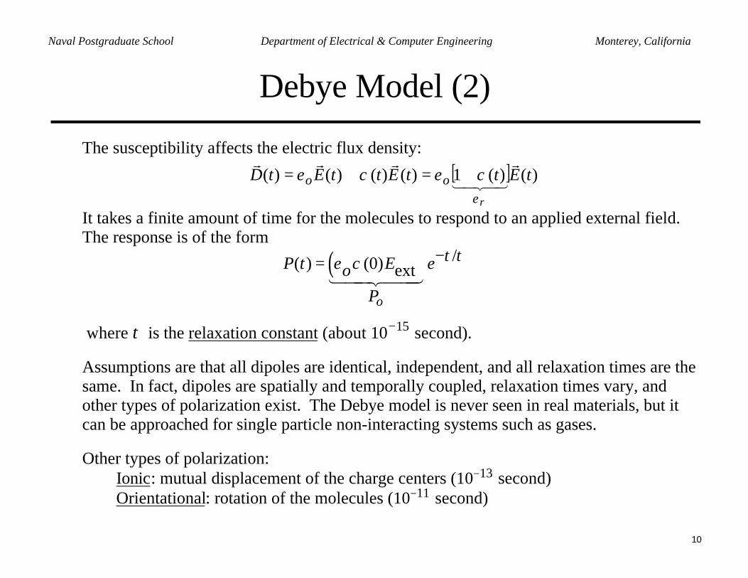
Naval Postgraduate School Department of Electrical & Computer Engineering Monterey, California
Debye Model (2)
The susceptibility affects the electric flux density:
[ ] )()(1)()()()( tEttEttEtDr
oorrrr
43421ε
χεχε +=+=
It takes a finite amount of time for the molecules to respond to an applied external field.The response is of the form
( ) /( ) (0) ext
o
tP t E eoP
τε χ −= 1442443
where τ is the relaxation constant (about 1510− second).
Assumptions are that all dipoles are identical, independent, and all relaxation times are thesame. In fact, dipoles are spatially and temporally coupled, relaxation times vary, andother types of polarization exist. The Debye model is never seen in real materials, but itcan be approached for single particle non-interacting systems such as gases.
Other types of polarization:Ionic: mutual displacement of the charge centers (10−13 second)Orientational: rotation of the molecules (10−11 second)
11
Naval Postgraduate School Department of Electrical & Computer Engineering Monterey, California
Debye Model (3)
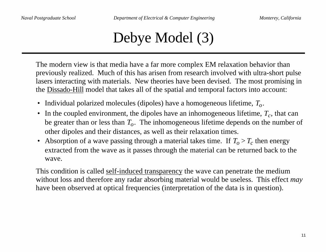
The modern view is that media have a far more complex EM relaxation behavior thanpreviously realized. Much of this has arisen from research involved with ultra-short pulselasers interacting with materials. New theories have been devised. The most promising inthe Dissado-Hill model that takes all of the spatial and temporal factors into account:
• Individual polarized molecules (dipoles) have a homogeneous lifetime, To.• In the coupled environment, the dipoles have an inhomogeneous lifetime, Tc, that can
be greater than or less than To. The inhomogeneous lifetime depends on the number ofother dipoles and their distances, as well as their relaxation times.
• Absorption of a wave passing through a material takes time. If To > Tc then energyextracted from the wave as it passes through the material can be returned back to thewave.
This condition is called self-induced transparency the wave can penetrate the mediumwithout loss and therefore any radar absorbing material would be useless. This effect mayhave been observed at optical frequencies (interpretation of the data is in question).
12
Naval Postgraduate School Department of Electrical & Computer Engineering Monterey, California
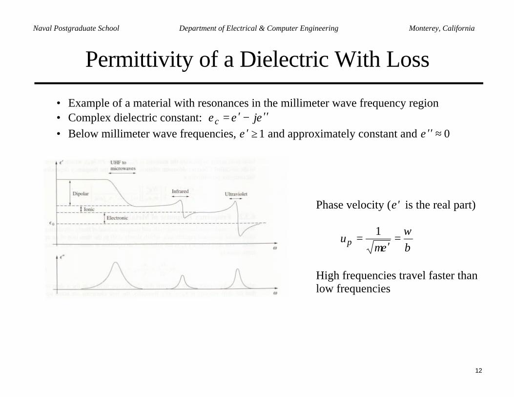
Permittivity of a Dielectric With Loss
• Example of a material with resonances in the millimeter wave frequency region• Complex dielectric constant: εεε ′′−′= jc• Below millimeter wave frequencies, 1≥′ε and approximately constant and 0≈′′ε
Phase velocity ( ′ ε is the real part)
βω
εµ=
′=
1pu
High frequencies travel faster thanlow frequencies
13
Naval Postgraduate School Department of Electrical & Computer Engineering Monterey, California
Precursors (1)
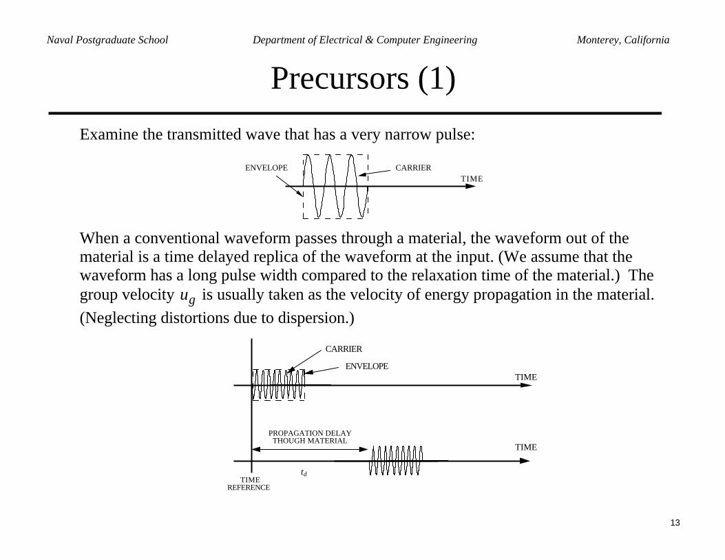
Examine the transmitted wave that has a very narrow pulse:
CARRIERENVELOPETIME
When a conventional waveform passes through a material, the waveform out of thematerial is a time delayed replica of the waveform at the input. (We assume that thewaveform has a long pulse width compared to the relaxation time of the material.) Thegroup velocity gu is usually taken as the velocity of energy propagation in the material.(Neglecting distortions due to dispersion.)
CARRIER
ENVELOPETIME
TIME
TIME REFERENCE
PROPAGATION DELAY THOUGH MATERIAL
td
14
Naval Postgraduate School Department of Electrical & Computer Engineering Monterey, California
Precursors (2)
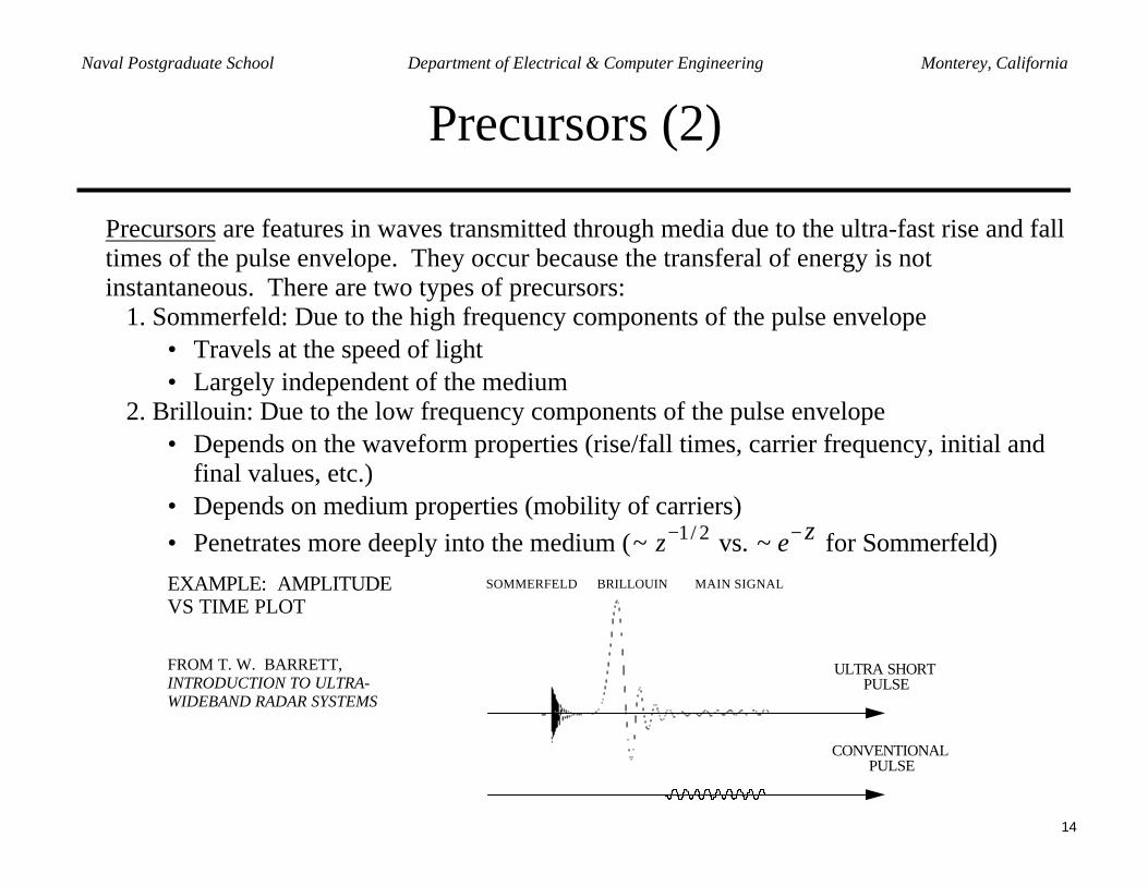
Precursors are features in waves transmitted through media due to the ultra-fast rise and falltimes of the pulse envelope. They occur because the transferal of energy is notinstantaneous. There are two types of precursors:
1. Sommerfeld: Due to the high frequency components of the pulse envelope• Travels at the speed of light• Largely independent of the medium
2. Brillouin: Due to the low frequency components of the pulse envelope• Depends on the waveform properties (rise/fall times, carrier frequency, initial and
final values, etc.)• Depends on medium properties (mobility of carriers)• Penetrates more deeply into the medium ( 2/1~ −z vs. ze−~ for Sommerfeld)EXAMPLE: AMPLITUDEVS TIME PLOT
FROM T. W. BARRETT,INTRODUCTION TO ULTRA-WIDEBAND RADAR SYSTEMS
SOMMERFELD BRILLOUIN MAIN SIGNAL
CONVENTIONAL PULSE
ULTRA SHORT PULSE
15
Naval Postgraduate School Department of Electrical & Computer Engineering Monterey, California
Propagation in Lossy Media (1)
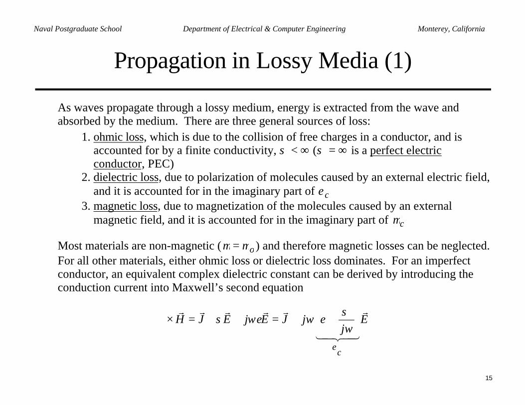
As waves propagate through a lossy medium, energy is extracted from the wave andabsorbed by the medium. There are three general sources of loss:
1. ohmic loss, which is due to the collision of free charges in a conductor, and isaccounted for by a finite conductivity, ∞<σ ( ∞=σ is a perfect electricconductor, PEC)
2. dielectric loss, due to polarization of molecules caused by an external electric field,and it is accounted for in the imaginary part of cε
3. magnetic loss, due to magnetization of the molecules caused by an externalmagnetic field, and it is accounted for in the imaginary part of cµ
Most materials are non-magnetic ( oµµ = ) and therefore magnetic losses can be neglected.For all other materials, either ohmic loss or dielectric loss dominates. For an imperfectconductor, an equivalent complex dielectric constant can be derived by introducing theconduction current into Maxwell’s second equation
Ej
jJEjEJH
c
r43421
rrrrr
ε
ωσ
εωωεσ
++=++=×∇
16
Naval Postgraduate School Department of Electrical & Computer Engineering Monterey, California
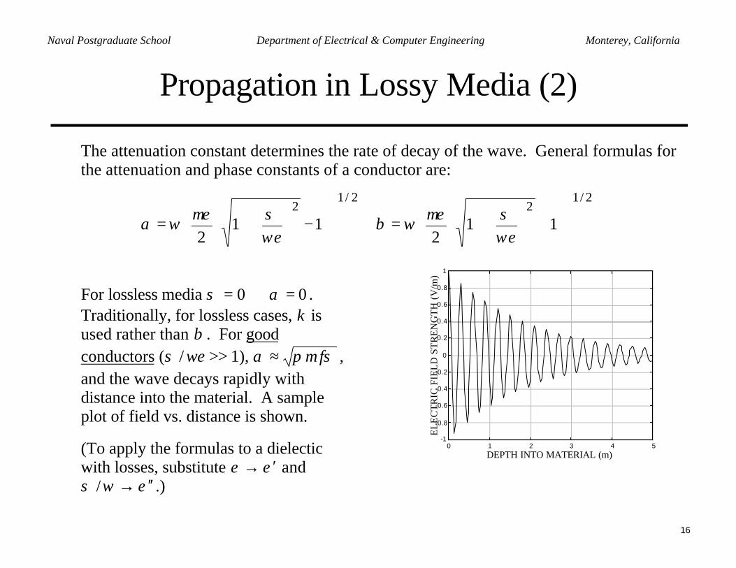
Propagation in Lossy Media (2)
The attenuation constant determines the rate of decay of the wave. General formulas forthe attenuation and phase constants of a conductor are:
2/12
2/12
112
112
+
+=
−
+=
ωεσµεωβ
ωεσµεωα
For lossless media 00 =⇒= ασ .Traditionally, for lossless cases, k isused rather than β . For goodconductors (σ / ωε >> 1), σµπα f≈ ,and the wave decays rapidly withdistance into the material. A sampleplot of field vs. distance is shown.
(To apply the formulas to a dielecticwith losses, substitute εε ′→ and
εωσ ′′→/ .)
EL
EC
TR
IC F
IEL
D S
TR
EN
GT
H (
V/m
)
DEPTH INTO MATERIAL (m)0 1 2 3 4 5
-1
-0.8
-0.6
-0.4
-0.2
0
0.2
0.4
0.6
0.8
1
17
Naval Postgraduate School Department of Electrical & Computer Engineering Monterey, California
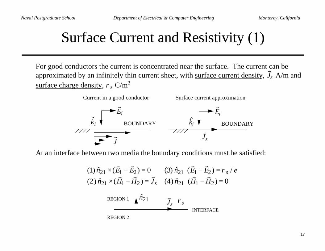
Surface Current and Resistivity (1)
For good conductors the current is concentrated near the surface. The current can beapproximated by an infinitely thin current sheet, with surface current density,
r J s A/m and
surface charge density, ρs C/m2
r E i
ˆ k i
r J
BOUNDARY
r E i
ˆ k i BOUNDARY
r J s
Current in a good conductor Surface current approximation
At an interface between two media the boundary conditions must be satisfied:
(1) ˆ n 21 × (
r E 1 −
r E 2 ) = 0 (3) ˆ n 21 ⋅ (
r E 1 −
r E 2 ) = ρs / ε
(2) ˆ n 21 × (r H 1 −
r H 2 ) =
r J s (4) ˆ n 21 ⋅(
r H 1 −
r H 2 ) = 0
REGION 2
REGION 1 r J s
ˆ n 21
INTERFACE
ρs
18
Naval Postgraduate School Department of Electrical & Computer Engineering Monterey, California
Surface Current and Resistivity (2)
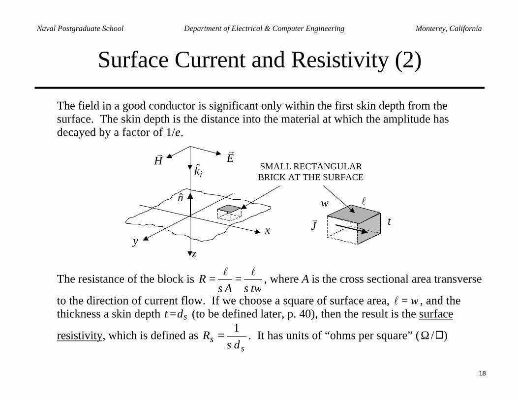
The field in a good conductor is significant only within the first skin depth from thesurface. The skin depth is the distance into the material at which the amplitude hasdecayed by a factor of 1/e.
xy
z
Hr E
rik
lw
tJr
SMALL RECTANGULARBRICK AT THE SURFACE
n
The resistance of the block is twA
Rσσll
== , where A is the cross sectional area transverse
to the direction of current flow. If we choose a square of surface area, w=l , and thethickness a skin depth st δ= (to be defined later, p. 40), then the result is the surface
resistivity, which is defined as s
sRσδ
1= . It has units of “ohms per square” ( /Ω )
19
Naval Postgraduate School Department of Electrical & Computer Engineering Monterey, California
Surface Current and Resistivity (3)
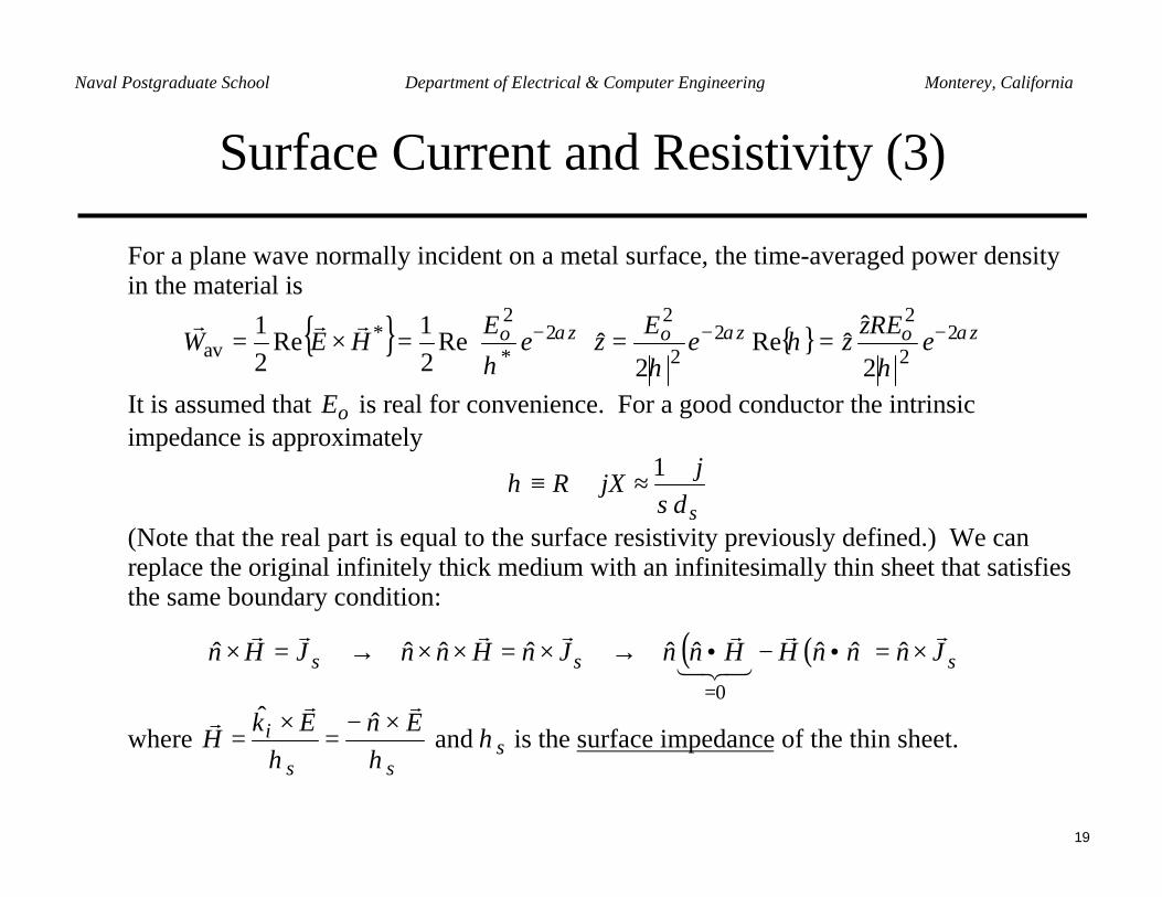
For a plane wave normally incident on a metal surface, the time-averaged power densityin the material is
zozozo eREz
zeE
zeE
HEW ααα
ηη
ηη2
2
22
2
22
*
2*
av2
ˆˆRe
2ˆRe
21
Re21 −−− ==
=×=rrr
It is assumed that oE is real for convenience. For a good conductor the intrinsicimpedance is approximately
s
jjXR
σδη
+≈+≡
1
(Note that the real part is equal to the surface resistivity previously defined.) We canreplace the original infinitely thick medium with an infinitesimally thin sheet that satisfiesthe same boundary condition:
( ) ( ) sss JnnnHHnnJnHnnJHnrr
321rrrrr
×=•−•→×=××→=×=
ˆˆˆˆˆˆˆˆˆ0
where ss
i EnEkH
ηη
rrr ×−=
×=
ˆˆ and sη is the surface impedance of the thin sheet.
20
Naval Postgraduate School Department of Electrical & Computer Engineering Monterey, California
Surface Current and Resistivity (4)
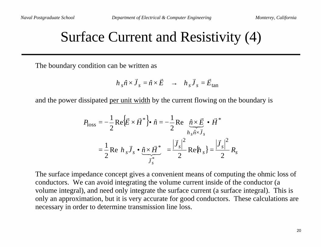
The boundary condition can be written as
tanˆˆ EJEnJn ssssrrrr
=→×=× ηη
and the power dissipated per unit width by the current flowing on the boundary is
ss
ss
J
ss
Jn
RJJ
HnJ
HEnnHEP
s
ss
2Re
2ˆRe
21
ˆRe21
ˆRe21
22*
*
ˆ
*loss
*
rr321rr
r321rrr
r
r
==
ו=
•×−=•×−=×
ηη
η
The surface impedance concept gives a convenient means of computing the ohmic loss ofconductors. We can avoid integrating the volume current inside of the conductor (avolume integral), and need only integrate the surface current (a surface integral). This isonly an approximation, but it is very accurate for good conductors. These calculations arenecessary in order to determine transmission line loss.
21
Naval Postgraduate School Department of Electrical & Computer Engineering Monterey, California
Circular Polarization (1)
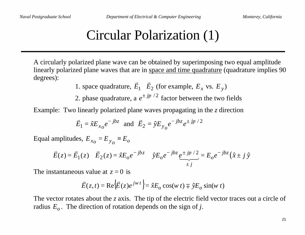
A circularly polarized plane wave can be obtained by superimposing two equal amplitudelinearly polarized plane waves that are in space and time quadrature (quadrature implies 90degrees):
1. space quadrature, 21 EErr
⊥ (for example, xE vs. yE )
2. phase quadrature, a 2/πje± factor between the two fields
Example: Two linearly polarized plane waves propagating in the z direction
zjox eExE β−= ˆ1
r and 2/
2 ˆ πβ jzjoy eeEyE ±−=
r
Equal amplitudes, ooyox EEE ≡=
( )yjxeEeeEyeExzEzEzE zjo
j
jzjo
zjo ˆˆˆˆ)()()( 2/
21 ±=+=+= −
±
±−− βπββ 321rrr
The instantaneous value at 0=z is
)sin(ˆ)cos(ˆ)(Re),( tEytExezEtzE ootj ωωω ∓rr
==
The vector rotates about the z axis. The tip of the electric field vector traces out a circle ofradius oE . The direction of rotation depends on the sign of j.
22
Naval Postgraduate School Department of Electrical & Computer Engineering Monterey, California
Circular Polarization (2)
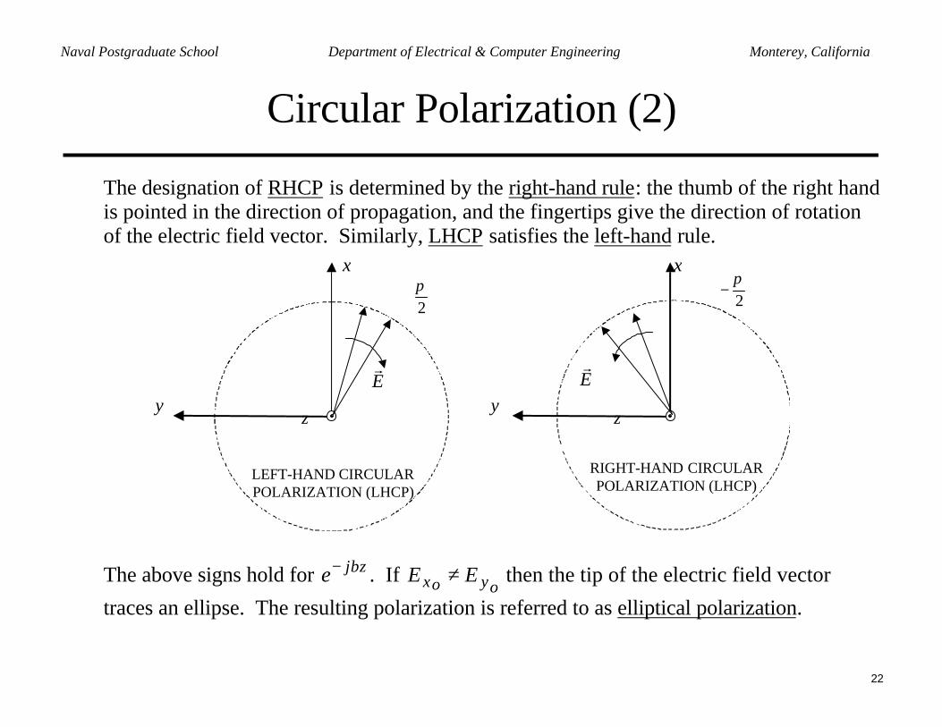
The designation of RHCP is determined by the right-hand rule: the thumb of the right handis pointed in the direction of propagation, and the fingertips give the direction of rotationof the electric field vector. Similarly, LHCP satisfies the left-hand rule.
x
yz
r E
LEFT-HAND CIRCULARPOLARIZATION (LHCP)
x
yz
r E
RIGHT-HAND CIRCULARPOLARIZATION (LHCP)
2π+ 2
π−
The above signs hold for zje β− . If oyox EE ≠ then the tip of the electric field vector
traces an ellipse. The resulting polarization is referred to as elliptical polarization.
23
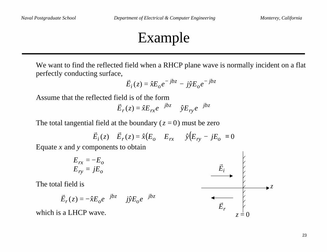
Naval Postgraduate School Department of Electrical & Computer Engineering Monterey, California
Example
We want to find the reflected field when a RHCP plane wave is normally incident on a flatperfectly conducting surface,
zjo
zjoi eEyjeExzE ββ −− −= ˆˆ)(
r
Assume that the reflected field is of the formzj
ryzj
rxr eEyeExzE ββ ++ += ˆˆ)(r
The total tangential field at the boundary ( 0=z ) must be zero
( ) ( ) 0ˆˆ)()( ≡−++=+ oryrxori jEEyEExzEzErr
Equate x and y components to obtain
ory
orxjEEEE
=−=
The total field is
zjo
zjor eEyjeExzE ββ ++ +−= ˆˆ)(
r
which is a LHCP wave.
iEr
rEr
z
0=z
24
Naval Postgraduate School Department of Electrical & Computer Engineering Monterey, California
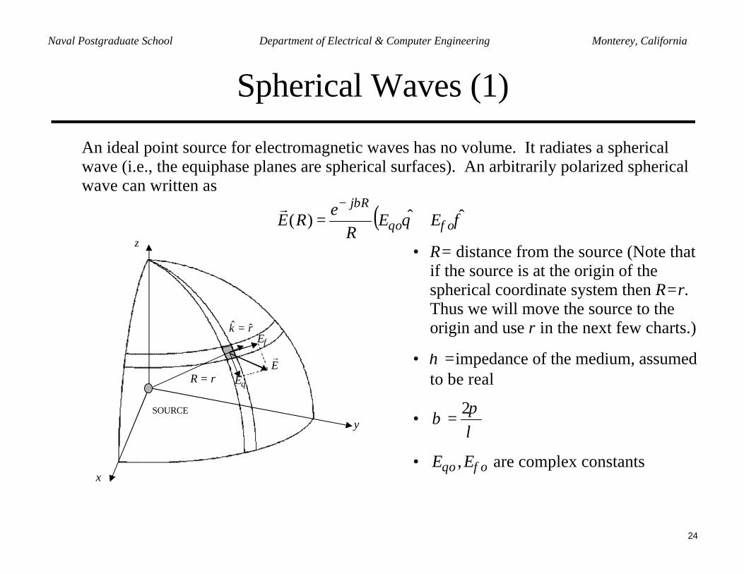
Spherical Waves (1)
An ideal point source for electromagnetic waves has no volume. It radiates a sphericalwave (i.e., the equiphase planes are spherical surfaces). An arbitrarily polarized sphericalwave can written as
( )φθ φθ
βˆˆ)( oo
RjEE
Re
RE +=−r
x
y
z
rk ˆˆ =
SOURCE
rR = θE
φE
Er
• R= distance from the source (Note thatif the source is at the origin of thespherical coordinate system then R=r.Thus we will move the source to theorigin and use r in the next few charts.)
• =η impedance of the medium, assumedto be real
• λπ
β2
=
• oo EE φθ , are complex constants
25
Naval Postgraduate School Department of Electrical & Computer Engineering Monterey, California
Spherical Waves (2)
Spherical waves are TEM, so the magnetic field intensity is
( ) ( )φθηη
φθ
η θφ
ββφθ ˆˆ
ˆˆˆ)(ˆ)( oo
rjrjoo EE
re
er
EErrEkrH +−=
+×=
×=
−−
rr
and the time-averaged Poynting vector (assuming oo EE φθ , are real)
( ) ( )( ) ( )( )rEE
r
EEEEr
rHrEW
oo
oooo
ˆ2
1
ˆˆˆˆ2
1)()(Re
21
222
2*
av
φθ
θφφθ
η
φθφθη
+=
+−×+=×=rrr
The power flowing through a spherical surface of radius r is
( ) ( )
( ) ( ) ( ) ( )
222 2av 2av
0 0
2 22 2
0
2
1 1 ˆ ˆ sin2
2 2sin
2
o oS
o o o o
P W ds E E r r r d dr
E E d E E
π π
θ φ
π
θ φ θ φ
θ θ φη
π πθ θ
η η
=
= = +
= + = +
∫∫ ∫ ∫
∫
rr i i
14243
26
Naval Postgraduate School Department of Electrical & Computer Engineering Monterey, California
Spherical Waves (3)
Note that the power spreads as 21
r (the “inverse square law”). We will see that a far field
region can be defined for any antenna. It is the region beyond a minimum distance, ffr ,where the wave becomes spherical with the following properties:
1. the wave propagates radially outward2. it is TEM (there are only θ and φ field components)
3. the field components vary as r1
At a large distance from the source of a spherical wave, the phase front becomes locallyplane.
SOURCE
FAR FIELD
ff r
SOURCE r
LOCALLY A GOODAPPROXIMATION TO
A PLANE WAVE
27
Naval Postgraduate School Department of Electrical & Computer Engineering Monterey, California
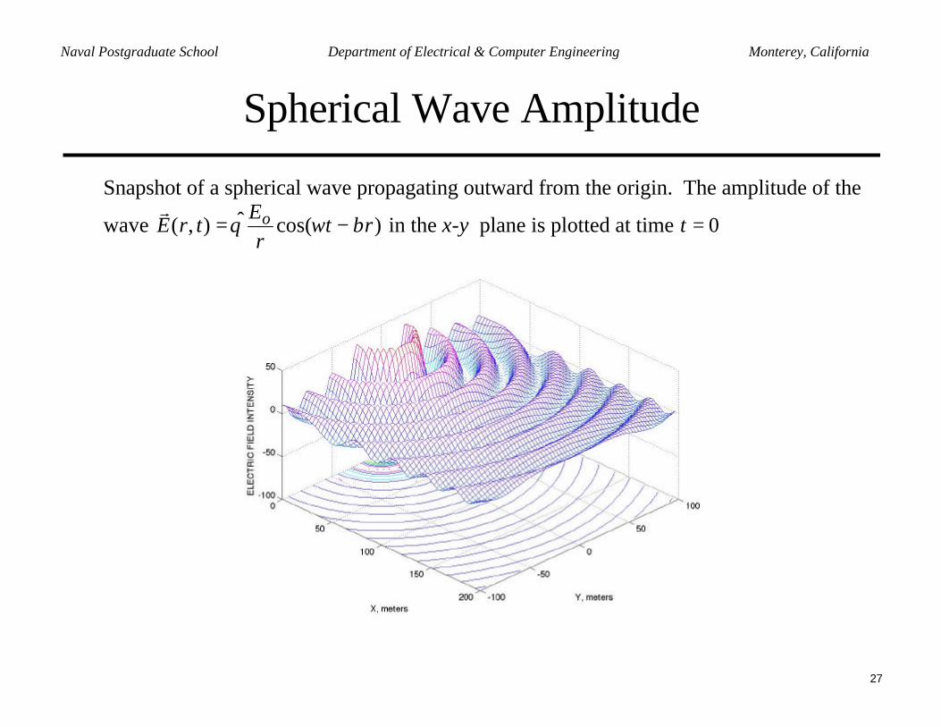
Spherical Wave Amplitude
Snapshot of a spherical wave propagating outward from the origin. The amplitude of the
wave )cos(ˆ),( rtr
EtrE o βωθ −=
r in the x-y plane is plotted at time t = 0
28
Naval Postgraduate School Department of Electrical & Computer Engineering Monterey, California
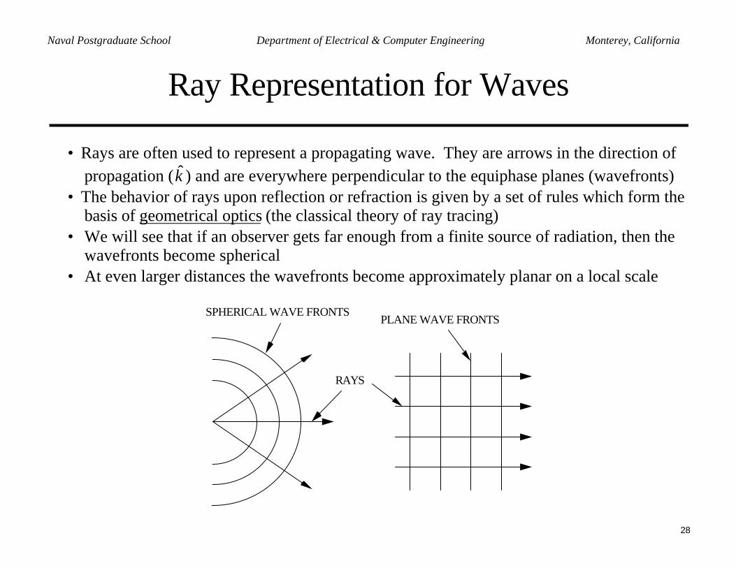
Ray Representation for Waves
• Rays are often used to represent a propagating wave. They are arrows in the direction ofpropagation ( k ) and are everywhere perpendicular to the equiphase planes (wavefronts)
• The behavior of rays upon reflection or refraction is given by a set of rules which form thebasis of geometrical optics (the classical theory of ray tracing)
• We will see that if an observer gets far enough from a finite source of radiation, then thewavefronts become spherical
• At even larger distances the wavefronts become approximately planar on a local scale
SPHERICAL WAVE FRONTSPLANE WAVE FRONTS
RAYS
29
Naval Postgraduate School Department of Electrical & Computer Engineering Monterey, California
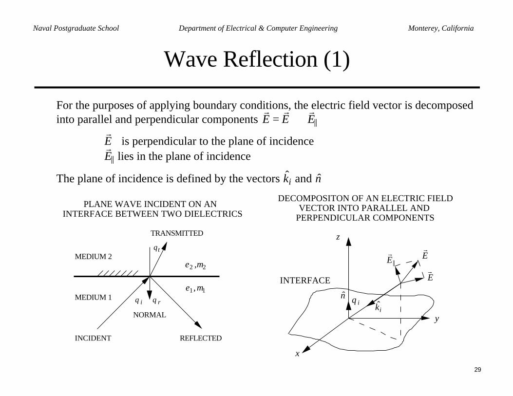
Wave Reflection (1)
For the purposes of applying boundary conditions, the electric field vector is decomposedinto parallel and perpendicular components
r E =
r E ⊥ +
r E ||
r E ⊥ is perpendicular to the plane of incidence
r E || lies in the plane of incidence
The plane of incidence is defined by the vectors ˆ k i and ˆ n
MEDIUM 2
MEDIUM 1
NORMAL
INCIDENT REFLECTED
TRANSMITTED
θ i θ r
θt
ε1, µ1
ε2 ,µ2
r E ⊥
r E ||
r E
x
y
z
ˆ n θ i
INTERFACE
ˆ k i
PLANE WAVE INCIDENT ON AN INTERFACE BETWEEN TWO DIELECTRICS
DECOMPOSITON OF AN ELECTRIC FIELD VECTOR INTO PARALLEL AND
PERPENDICULAR COMPONENTS
30
Naval Postgraduate School Department of Electrical & Computer Engineering Monterey, California
Wave Reflection (2)
θi
θrθt
εr µr
µoεo
FREE SPACE DIELECTRIC
ˆ n
ˆ k i
ˆ k r
iEr
rEr
tEr z
iHr
rHr
tHr
tk
θi
θrθt
εr µr
µoεo
FREE SPACE DIELECTRIC
ˆ n
ˆ k i
ˆ k r
iEr
rEr
tEr
iHr
rHr
tHr
tk
z
PERPENDICULAR POLARIZATION PARALLEL POLARIZATION
The incident fields ( ii HErr
, ) are known in each case. We can write expressions for thereflected and transmitted fields ( rr HE
rr, ) and ( tt HE
rr, ), and then apply the boundary
conditions at 0=z :( ) ( )
tantan tri EEErrr
=+ and ( ) ( )tantan tri HHH
rrr=+
There is enough information to solve for the coefficients of the reflected and transmittedwaves.
31
Naval Postgraduate School Department of Electrical & Computer Engineering Monterey, California
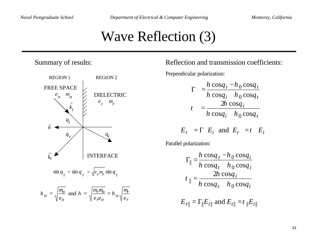
Wave Reflection (3)
Summary of results:
REGION 1 REGION 2
θi
θr θt
εr µr
µoεo
FREE SPACEDIELECTRIC
INTERFACE
ˆ n
ˆ k i
ˆ k r
trrriθθθ µε sinsinsin ==
o
oo ε
µη = and
r
ro
or
orεµ
ηεεµµ
η ==
Reflection and transmission coefficients:Perpendicular polarization:
and
coscoscos2
coscoscoscos
0
0
0
⊥⊥⊥⊥⊥⊥
⊥
⊥
=Γ=
+=
+−
=Γ
itir
ti
i
ti
ti
EEEE τ
θηθηθη
τ
θηθηθηθη
Parallel polarization:
||||||||||||
0||
0
0||
and
coscoscos2
coscoscoscos
itir
it
i
it
it
EEEE τ
θηθηθη
τ
θηθηθηθη
=Γ=
+=
+−
=Γ
32
Naval Postgraduate School Department of Electrical & Computer Engineering Monterey, California
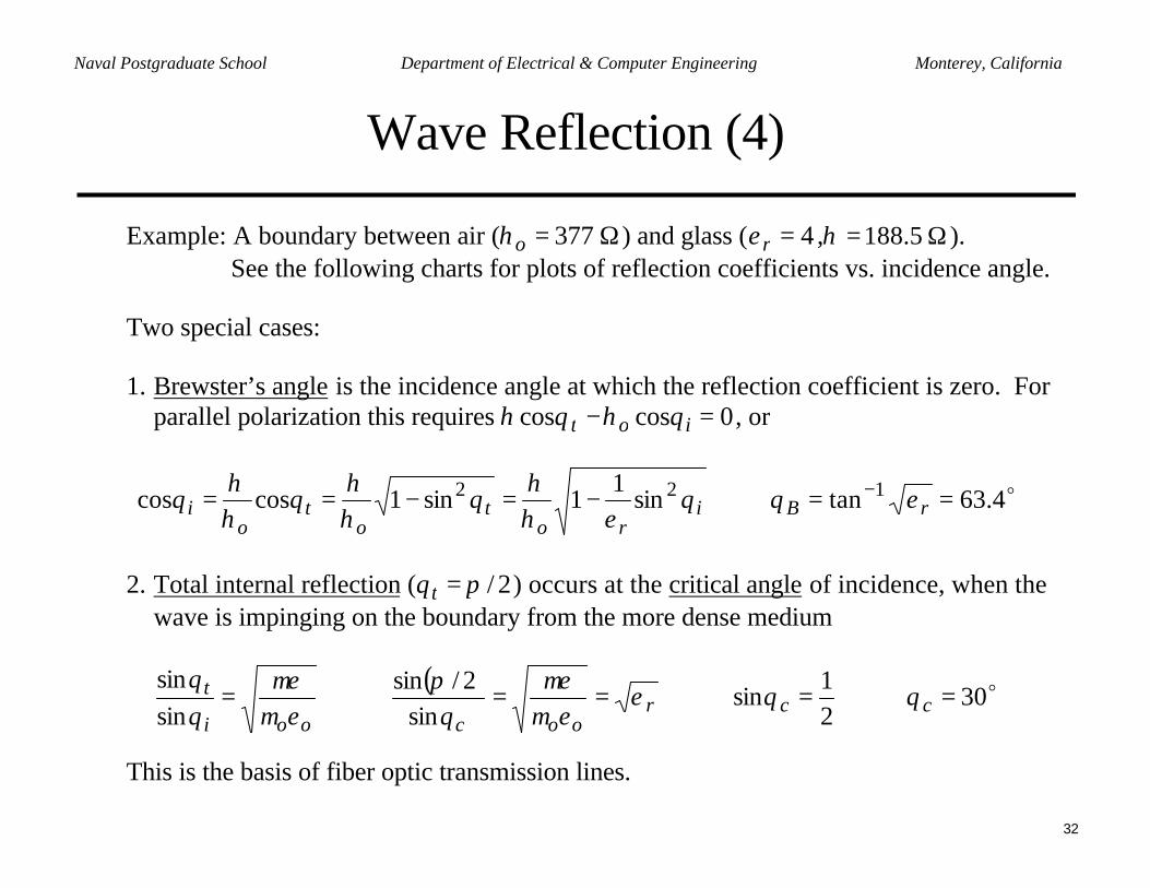
Wave Reflection (4)
Example: A boundary between air ( Ω= 377oη ) and glass ( 4=rε , Ω= 5.188η ).See the following charts for plots of reflection coefficients vs. incidence angle.
Two special cases:
1. Brewster’s angle is the incidence angle at which the reflection coefficient is zero. Forparallel polarization this requires 0coscos =− iot θηθη , or
o4.63tansin1
1sin1coscos 122 ==⇒−=−== −rBi
rot
ot
oi εθθ
εηη
θηη
θηη
θ
2. Total internal reflection ( 2/πθ =t ) occurs at the critical angle of incidence, when thewave is impinging on the boundary from the more dense medium
( ) o3021
sinsin
2/sinsinsin
=⇒=⇒==⇒= ccroocooi
t θθεεµ
µεθ
πεµ
µεθθ
This is the basis of fiber optic transmission lines.
33
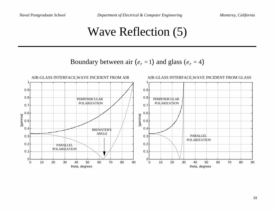
Naval Postgraduate School Department of Electrical & Computer Engineering Monterey, California
Wave Reflection (5)
Boundary between air (εr = 1) and glass (εr = 4)
0 10 20 30 40 50 60 70 80 900
0.1
0.2
0.3
0.4
0.5
0.6
0.7
0.8
0.9
1
theta, degrees
|gam
ma|
PARALLEL POLARIZATION
PERPENDICULAR POLARIZATION
AIR-GLASS INTERFACE,WAVE INCIDENT FROM GLASSAIR-GLASS INTERFACE,WAVE INCIDENT FROM AIR
0 10 20 30 40 50 60 70 80 900
0.1
0.2
0.3
0.4
0.5
0.6
0.7
0.8
0.9
1
theta, degrees
|gam
ma|
BREWSTER'S ANGLE
PERPENDICULAR POLARIZATION
PARALLEL POLARIZATION
34
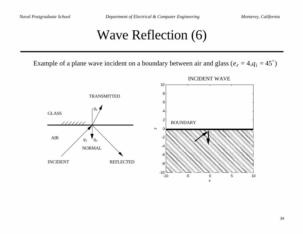
Naval Postgraduate School Department of Electrical & Computer Engineering Monterey, California
Wave Reflection (6)
Example of a plane wave incident on a boundary between air and glass (εr = 4, θi = 45o)
-10 -5 0 5 10-10
-8
-6
-4
-2
0
2
4
6
8
10
x
z
BOUNDARY
INCIDENT WAVE
GLASS
AIR
NORMAL
INCIDENT REFLECTED
TRANSMITTED
θi θr
θt
35
Naval Postgraduate School Department of Electrical & Computer Engineering Monterey, California
Wave Reflection (7)
Example of a plane wave reflection: reflected and transmitted waves (εr = 4, θi = 45o)
-10 -5 0 5 10-10
-8
-6
-4
-2
0
2
4
6
8
10
x
z
BOUNDARY
REFLECTED WAVE
-10 -5 0 5 10-10
-8
-6
-4
-2
0
2
4
6
8
10
x
z
BOUNDARY
TRANSMITTED WAVE
36
Naval Postgraduate School Department of Electrical & Computer Engineering Monterey, California
Wave Reflection (8)
Example of a plane wave reflection: total field
z
-10 -5 0 5 10-10
-8
-6
-4
-2
0
2
4
6
8
10
x
BOUNDARY
• The total field in region 1 is the sum of theincident and reflected fields
• If region 2 is more dense than region 1(i.e., εr2 > εr1) the transmitted wave isrefracted towards the normal
• If region 1 is more dense than region 2(i.e., εr1 > εr2) the transmitted wave isrefracted away from the normal
37
Naval Postgraduate School Department of Electrical & Computer Engineering Monterey, California
Example (1)
An aircraft is attempting to communicate with a submerged submarine directly below. Thefrequency is 0.5 MHz and the power density of the normally incident wave at the oceansurface is 12 kW/ 2m . The receiver on the submarine requires 0.1 V/mµ to establish areliable link. What is the maximum depth for communication?
AIR
OCEAN
0,, =σεµ oo
S/m 4,72, == σεµ roz
0=zik
tk
iEr
tEr
iHr
tHr
x
The phasor expression for the incident plane wave is zjoi
oeExzE β−= ˆ)(r
where
oooo λ
πεµωβ
2== , 600
105.0
1036
8=
×
×==fc
oλ m. The time-averaged power density is
given by the Poynting vector, )()(21
)( *av zHzEzW iii
rrr×=
38
Naval Postgraduate School Department of Electrical & Computer Engineering Monterey, California
Example (2)
At the ocean surface, z=0, and from the information provided we can solve for oE
3008)377)(2)(1012(W/m10122
)( 32232
av =⇒×=⇒×≡= ooo
o EEE
zWi η
r V/m
Below the ocean surface the electric field is given by zot eExzE γτ −= ˆ)(
r, where the
transmission coefficient is determined from the Fresnel formulas
0
0ηηηη
+−
=Γ , and oηη
ητ
+=Γ+=
21 .
To evaluate this we need the impedance of seawater
−
=−
==
ωεεσ
εε
µ
ωσ
ε
µεµ
η
roro
oo
c jj 1
Note that 12000)72)(1085.8)(105(2
4125
>>=××
=−πωεε
σ
ro which is typical of a good
conductor. Thus we drop the 1 in the denominator for good conductors.
39
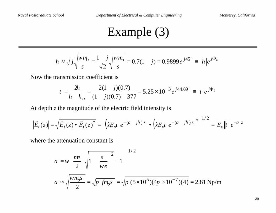
Naval Postgraduate School Department of Electrical & Computer Engineering Monterey, California
Example (3)
ηησ
ωµσ
ωµη Φ≡=+=
+=≈ jjoo eej
jj
o459899.0)1(7.02
1
Now the transmission coefficient is
ττηη
ητ Φ− ≡×=
+++
=+
= jj
oee
jj o89.4431025.5
377)7.0)(1()7.0)(1(22
At depth z the magnitude of the electric field intensity is
( ) ( ) zo
zjo
zjottt eEeExeExzEzEzE αβαβα τττ −+−+− =
•=•=
2/1*)()(* ˆˆ)()()(rrr
where the attenuation constant is
Np/m 81.2)4)(104)(105(2
112
75
2/12
=××==≈
−
+=
−ππσµπσωµ
α
ωεσµε
ωα
oo f
40
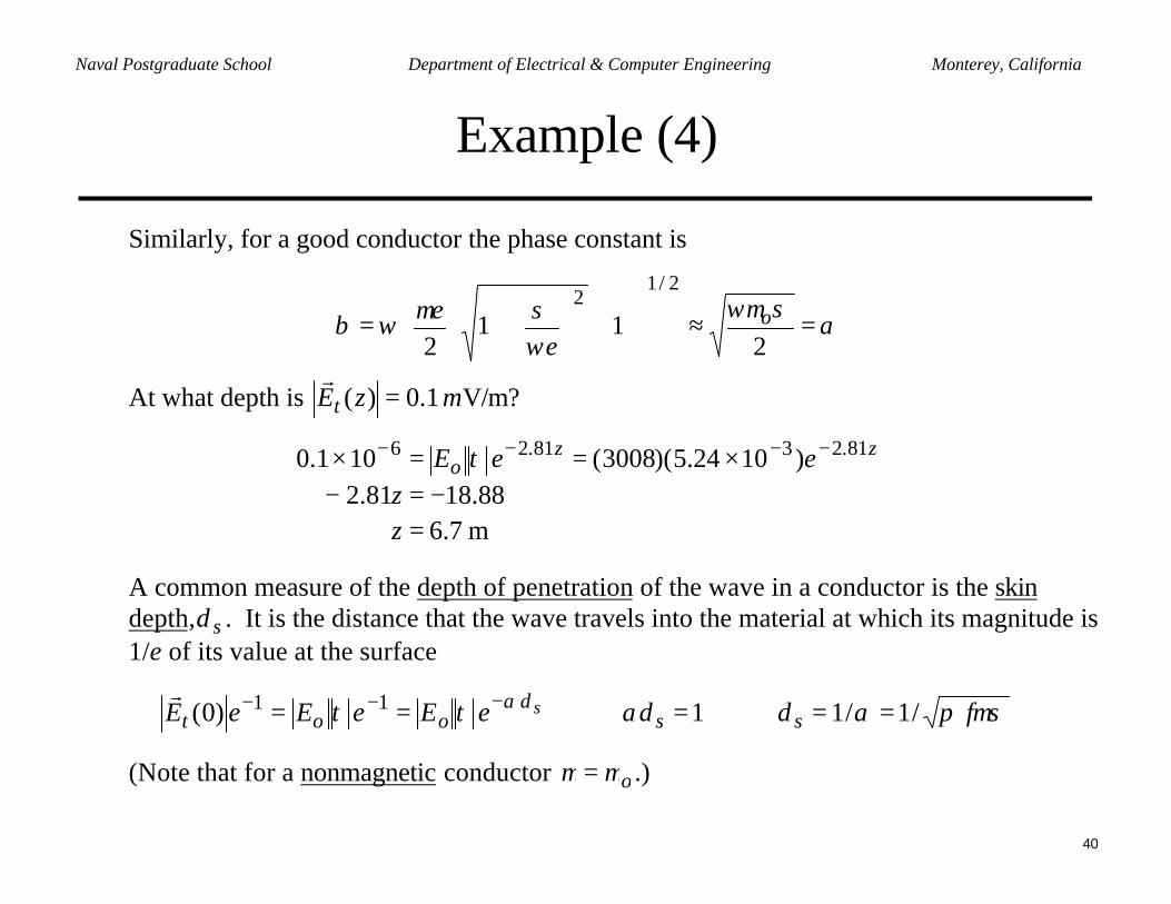
Naval Postgraduate School Department of Electrical & Computer Engineering Monterey, California
Example (4)
Similarly, for a good conductor the phase constant is
ασωµ
ωεσµεωβ =≈
+
+=
211
2
2/12
o
At what depth is µ1.0)( =zEtr
V/m?
m 7.688.1881.2
)1024.5)(3008(101.0 81.2381.26
=−=−
×==× −−−−
zz
eeE zzo τ
A common measure of the depth of penetration of the wave in a conductor is the skindepth, sδ . It is the distance that the wave travels into the material at which its magnitude is1/e of its value at the surface
µσπαδαδττ δα feEeEeE ssoots /1/11)0( 11 ==⇒=⇒== −−−r
(Note that for a nonmagnetic conductor oµµ = .)
41
Naval Postgraduate School Department of Electrical & Computer Engineering Monterey, California
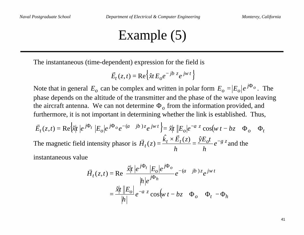
Example (5)
The instantaneous (time-dependent) expression for the field is
tjzjot eeExtzE ωβτ −= ˆRe),(
r
Note that in general oE can be complex and written in polar form .ojoo eEE Φ= The
phase depends on the altitude of the transmitter and the phase of the wave upon leavingthe aircraft antenna. We can not determine oΦ from the information provided, andfurthermore, it is not important in determining whether the link is established. Thus,
( )ταωβα βωττ τ Φ+Φ+−== −+−ΦΦ
oz
otjzjj
oj
t zteExeeeEextzE o cosˆˆRe),( )(r
The magnetic field intensity phasor is zottt e
EyzEkzH γ
ητ
η−=
×=
ˆ)(ˆ)(
rrand the
instantaneous value
( )ητα
ωβα
βωη
τη
τη
τ
Φ−Φ+Φ+−=
=
−
+−Φ
ΦΦ
ozo
tjzjj
jo
j
t
zteEx
eee
eEextzH
o
cosˆ
ˆRe),( )(r
42
Naval Postgraduate School Department of Electrical & Computer Engineering Monterey, California
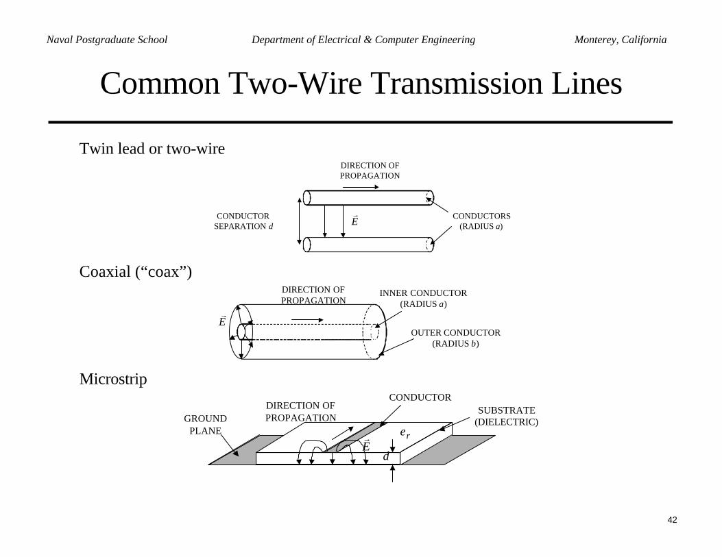
Common Two-Wire Transmission Lines
Twin lead or two-wire
Er
DIRECTION OFPROPAGATION
CONDUCTORS(RADIUS a)
CONDUCTORSEPARATION d
Coaxial (“coax”)
Er
DIRECTION OFPROPAGATION
INNER CONDUCTOR(RADIUS a)
OUTER CONDUCTOR(RADIUS b)
Microstrip
SUBSTRATE(DIELECTRIC)GROUND
PLANE
CONDUCTOR
Er
DIRECTION OFPROPAGATION
rε
d
43
Naval Postgraduate School Department of Electrical & Computer Engineering Monterey, California
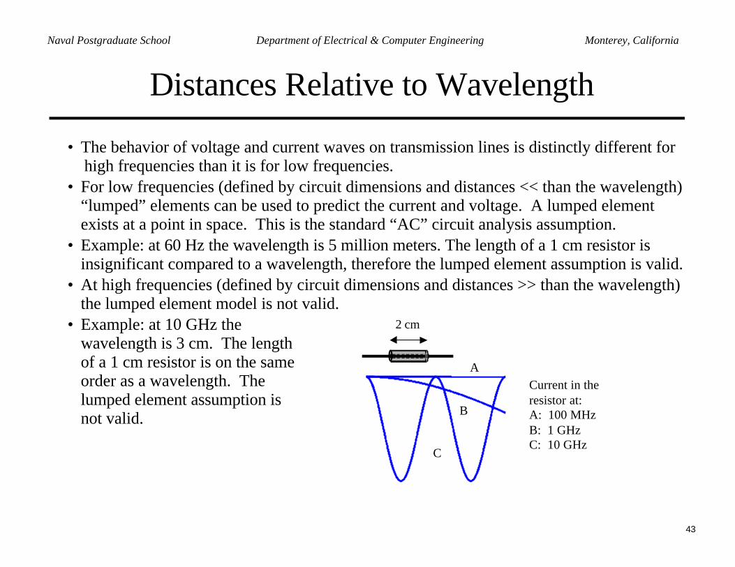
Distances Relative to Wavelength
• The behavior of voltage and current waves on transmission lines is distinctly different forhigh frequencies than it is for low frequencies.
• For low frequencies (defined by circuit dimensions and distances << than the wavelength)“lumped” elements can be used to predict the current and voltage. A lumped elementexists at a point in space. This is the standard “AC” circuit analysis assumption.
• Example: at 60 Hz the wavelength is 5 million meters. The length of a 1 cm resistor isinsignificant compared to a wavelength, therefore the lumped element assumption is valid.
• At high frequencies (defined by circuit dimensions and distances >> than the wavelength)the lumped element model is not valid.
• Example: at 10 GHz thewavelength is 3 cm. The lengthof a 1 cm resistor is on the sameorder as a wavelength. Thelumped element assumption isnot valid.
2 cm
Current in the resistor at:A: 100 MHzB: 1 GHzC: 10 GHz
B
C
A
44
Naval Postgraduate School Department of Electrical & Computer Engineering Monterey, California
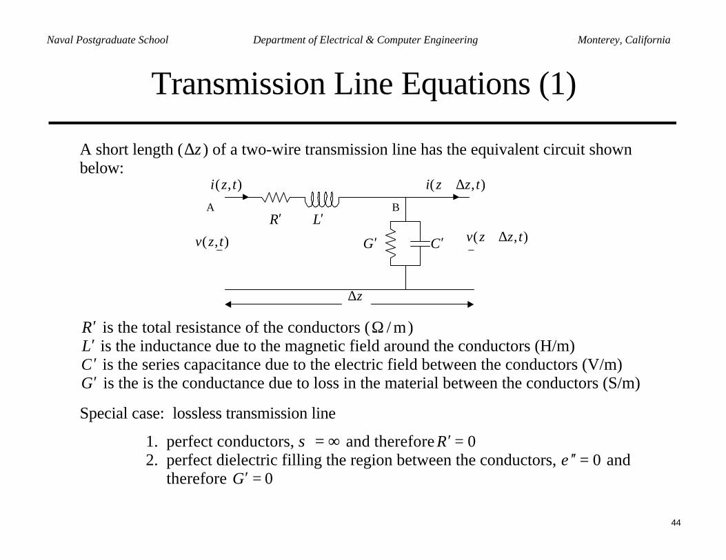
Transmission Line Equations (1)
A short length ( z∆ ) of a two-wire transmission line has the equivalent circuit shownbelow:
z∆
L′
C′
R′
G′
),( tzi ),( tzzi ∆+
),( tzv ),( tzzv ∆++ +
−−
BA
R′ is the total resistance of the conductors ( m/Ω )L′ is the inductance due to the magnetic field around the conductors (H/m)C ′ is the series capacitance due to the electric field between the conductors (V/m)G′ is the is the conductance due to loss in the material between the conductors (S/m)
Special case: lossless transmission line
1. perfect conductors, ∞=σ and therefore 0=′R2. perfect dielectric filling the region between the conductors, 0=′′ε and
therefore 0=′G
45
Naval Postgraduate School Department of Electrical & Computer Engineering Monterey, California
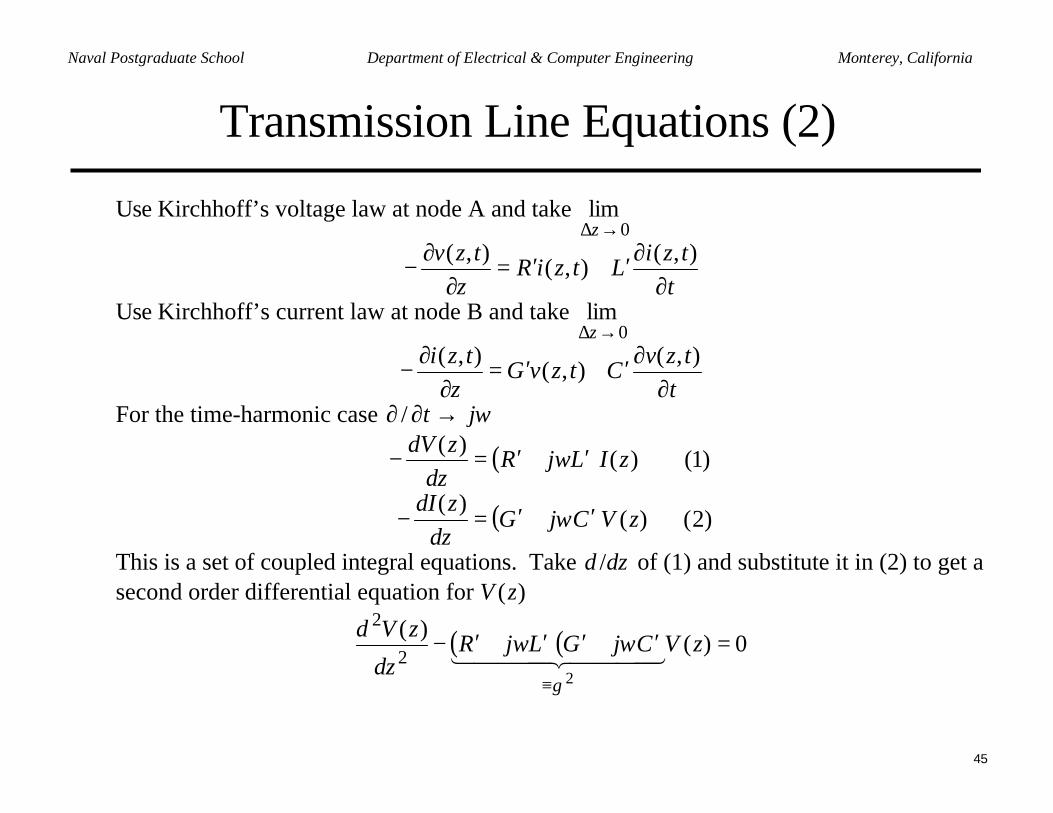
Transmission Line Equations (2)
Use Kirchhoff’s voltage law at node A and take 0
lim→∆z
ttzi
LtziRz
tzv∂
∂′+′=∂
∂−
),(),(
),(
Use Kirchhoff’s current law at node B and take 0
lim→∆z
ttzv
CtzvGz
tzi∂
∂′+′=∂
∂−
),(),(
),(
For the time-harmonic case ωjt →∂∂ /
( )
( ) )2()()(
)1()()(
zVCjGdz
zdI
zILjRdz
zdV
′+′=−
′+′=−
ω
ω
This is a set of coupled integral equations. Take dzd / of (1) and substitute it in (2) to get asecond order differential equation for )(zV
( )( ) 0)()(
22
2=′+′′+′−
≡
zVCjGLjRdz
zVd4444 34444 21
γ
ωω
46
Naval Postgraduate School Department of Electrical & Computer Engineering Monterey, California
Transmission Line Equations (3)
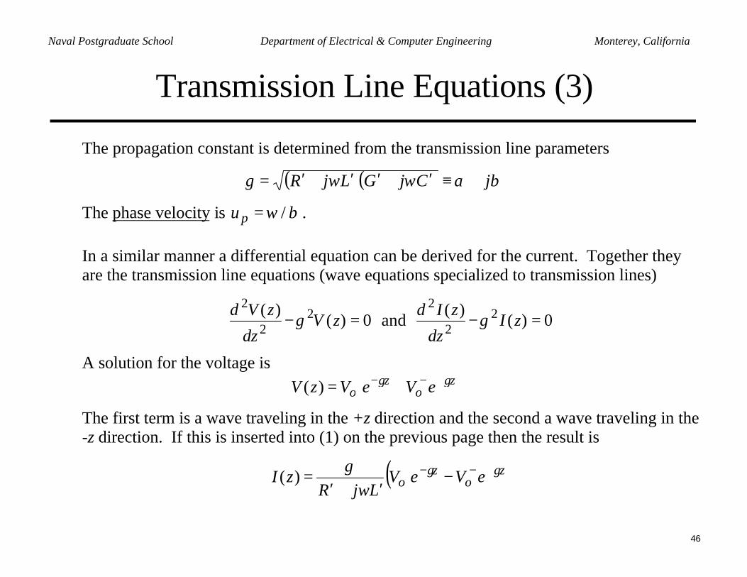
The propagation constant is determined from the transmission line parameters
( )( ) βαωωγ jCjGLjR +≡′+′′+′=
The phase velocity is βω /=pu .
In a similar manner a differential equation can be derived for the current. Together theyare the transmission line equations (wave equations specialized to transmission lines)
0)()( 2
2
2=− zV
dz
zVdγ and 0)(
)( 22
2=− zI
dz
zIdγ
A solution for the voltage isz
oz
o eVeVzV γγ +−−+ +=)(
The first term is a wave traveling in the +z direction and the second a wave traveling in the-z direction. If this is inserted into (1) on the previous page then the result is
( )zo
zo eVeV
LjRzI γγ
ωγ +−−+ −
′+′=)(
47
Naval Postgraduate School Department of Electrical & Computer Engineering Monterey, California
Transmission Line Equations (4)
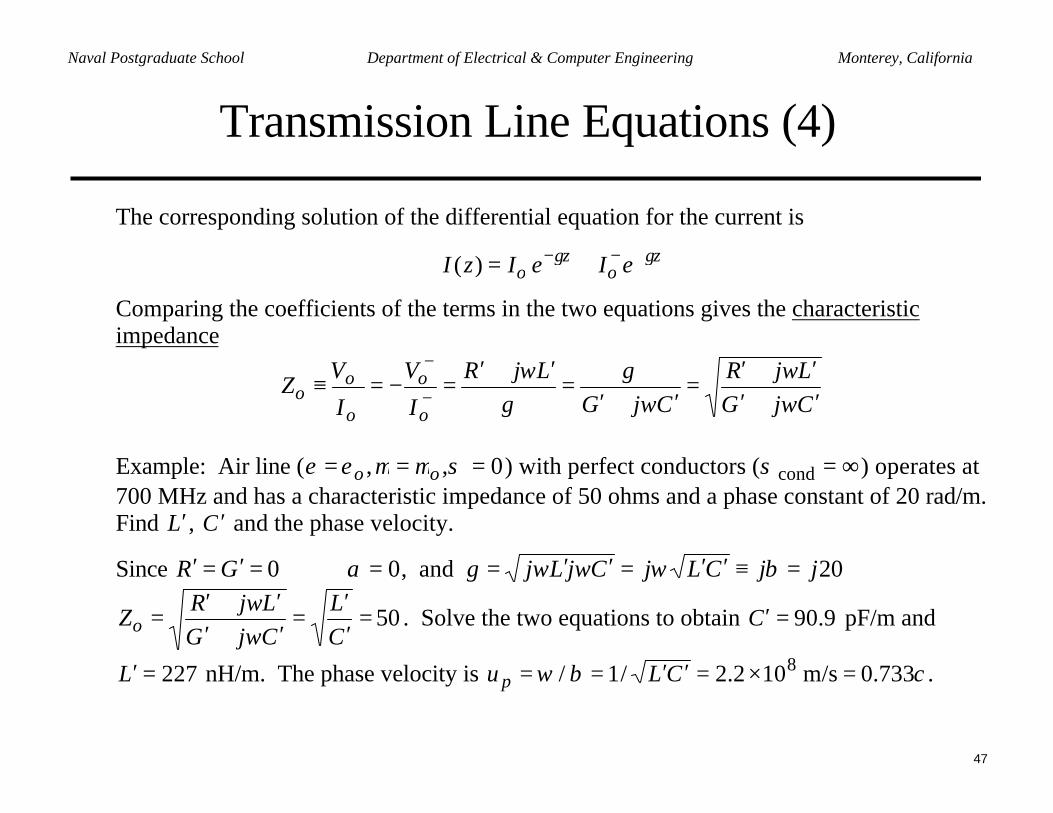
The corresponding solution of the differential equation for the current is
zo
zo eIeIzI γγ +−−+ +=)(
Comparing the coefficients of the terms in the two equations gives the characteristicimpedance
CjGLjR
CjGLjR
I
V
I
VZ
o
o
o
oo ′+′
′+′=
′+′=
′+′=−=≡ −
−
+
+
ωω
ωγ
γω
Example: Air line ( 0,, === σµµεε oo ) with perfect conductors ( ∞=condσ ) operates at700 MHz and has a characteristic impedance of 50 ohms and a phase constant of 20 rad/m.Find L′, C ′ and the phase velocity.
Since 00 =⇒=′=′ αGR , and 20jjCLjCjLj =≡′′=′′= βωωωγ
50=′′
=′+′′+′
=CL
CjGLjR
Zo ωω
. Solve the two equations to obtain 9.90=′C pF/m and
227=′L nH/m. The phase velocity is cCLu p 0.733m/s 102.2/1/ 8 =×=′′== βω .
48
Naval Postgraduate School Department of Electrical & Computer Engineering Monterey, California
Transmission Line Equations (5)
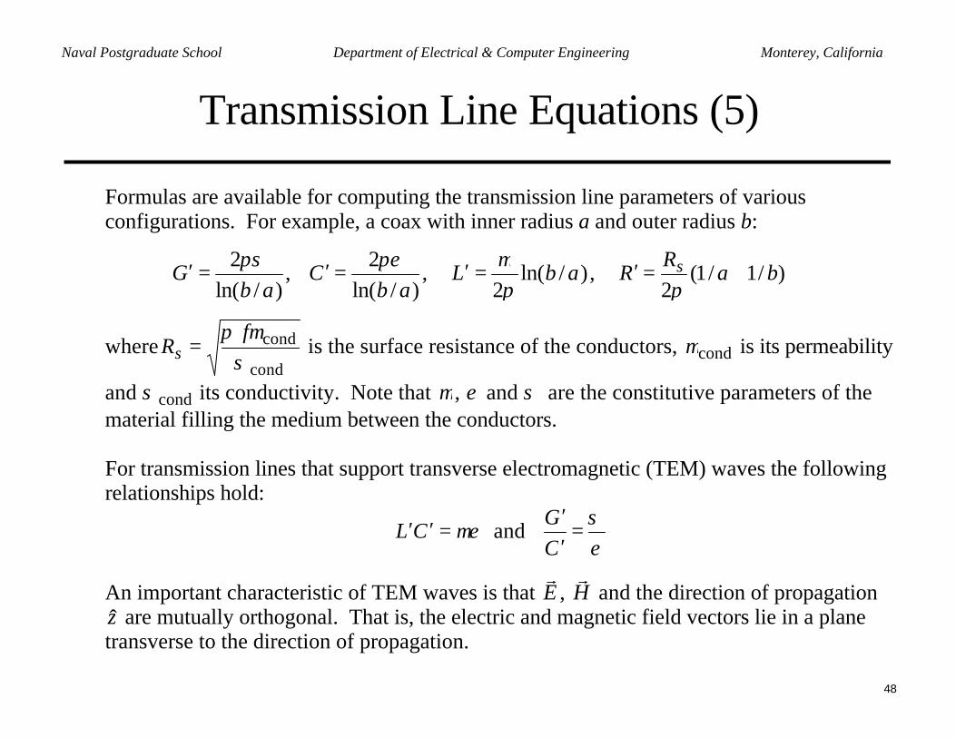
Formulas are available for computing the transmission line parameters of variousconfigurations. For example, a coax with inner radius a and outer radius b:
)/ln(2
abG
πσ=′ ,
)/ln(2
abC
πε=′ , )/ln(
2abL
πµ
=′ , )/1/1(2
baR
R s +=′π
wherecond
condσ
µπ fRs = is the surface resistance of the conductors, condµ is its permeability
and condσ its conductivity. Note that µ , ε and σ are the constitutive parameters of thematerial filling the medium between the conductors.
For transmission lines that support transverse electromagnetic (TEM) waves the followingrelationships hold:
µε=′′CL and εσ
=′′
CG
An important characteristic of TEM waves is that Er
, Hr
and the direction of propagationz are mutually orthogonal. That is, the electric and magnetic field vectors lie in a planetransverse to the direction of propagation.
49
Naval Postgraduate School Department of Electrical & Computer Engineering Monterey, California
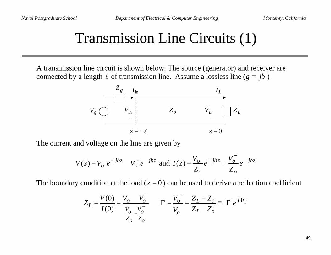
Transmission Line Circuits (1)
A transmission line circuit is shown below. The source (generator) and receiver areconnected by a length l of transmission line. Assume a lossless line ( βγ j= )
l−=z 0=z
gZ
LZLVgV oZinV
inI LI
+
−
+
−
+
−
The current and voltage on the line are given by
zjo
zjo eVeVzV ββ +−−+ +=)( and zj
o
ozj
o
o eZV
eZV
zI ββ +−
−+
−=)(
The boundary condition at the load ( 0=z ) can be used to derive a reflection coefficient
(0)(0)
jo o o L oL
V V L oo o oZ Zo o
V V V Z ZVZ e
I Z ZVΓ
+ − −Φ
+ − +−
+ −= = ⇒ Γ = = ≡ Γ
+
50
Naval Postgraduate School Department of Electrical & Computer Engineering Monterey, California
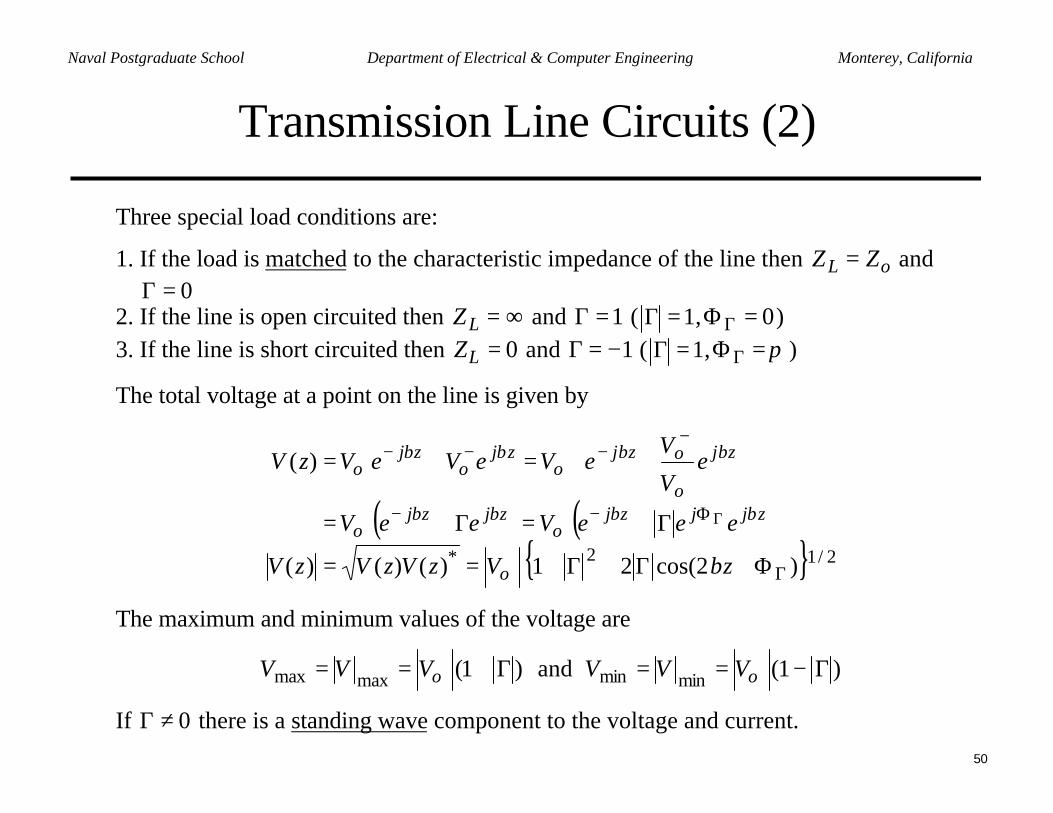
Transmission Line Circuits (2)
Three special load conditions are:
1. If the load is matched to the characteristic impedance of the line then oL ZZ = and0=Γ
2. If the line is open circuited then ∞=LZ and 1=Γ ( 1=Γ , 0=ΦΓ )3. If the line is short circuited then 0=LZ and 1−=Γ ( 1=Γ , π=ΦΓ )
The total voltage at a point on the line is given by
( ) ( ) 2/12* )2cos(21)()()(
)(
Γ+
Φ−+−+
+
−−+−−+
Φ+Γ+Γ+==
Γ+=Γ+=
+=+=
Γ
zVzVzVzV
eeeVeeV
eV
VeVeVeVzV
o
zjjzjo
zjzjo
zj
o
ozjo
zjo
zjo
β
ββββ
ββββ
The maximum and minimum values of the voltage are
)1(maxmax Γ+== +oVVV and )1(minmin Γ−== +
oVVV
If 0≠Γ there is a standing wave component to the voltage and current.
51
Naval Postgraduate School Department of Electrical & Computer Engineering Monterey, California
Transmission Line Circuits (3)
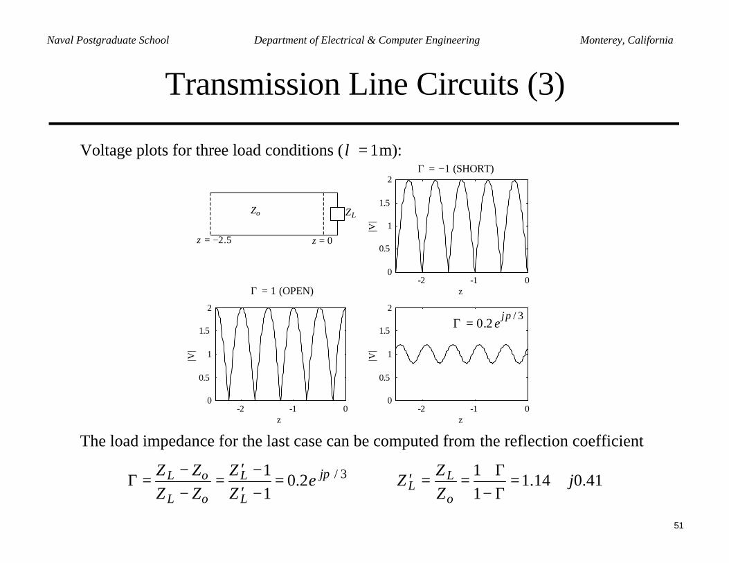
Voltage plots for three load conditions ( 1=λ m):
-2 -1 00
0.5
1
1.5
2
z
|V|
-2 -1 00
0.5
1
1.5
2
z
|V|
-2 -1 00
0.5
1
1.5
2
z
|V|
Γ = 1 (OPEN)
Γ = 0.2 ejπ / 3
Γ = −1 (SHORT)
z = −2.5 z = 0
LZZo
The load impedance for the last case can be computed from the reflection coefficient
41.014.111
2.011 3/ j
ZZ
ZeZZ
ZZZZ
o
LL
j
L
L
oL
oL +=Γ−Γ+
==′⇒=−′−′
=−−
=Γ π
52
Naval Postgraduate School Department of Electrical & Computer Engineering Monterey, California
Transmission Line Circuits (4)
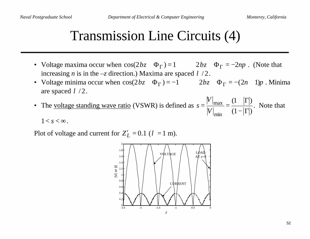
• Voltage maxima occur when πββ nzz 221)2cos( −=Φ+⇒=Φ+ ΓΓ . (Note thatincreasing n is in the –z direction.) Maxima are spaced 2/λ .
• Voltage minima occur when πββ )12(21)2cos( +−=Φ+⇒−=Φ+ ΓΓ nzz . Minimaare spaced 2/λ .
• The voltage standing wave ratio (VSWR) is defined as )1()1(
min
max
Γ−Γ+
==V
Vs . Note that
∞<< s1 .
Plot of voltage and current for 1.0=′LZ ( 1=λ m).
-2.5 -2 -1.5 -1 -0.5 00
0.2
0.4
0.6
0.8
1
1.2
1.4
1.6
1.8
2
z
|V| o
r |I|
VOLTAGE
CURRENT
LOADAT z=0
53
Naval Postgraduate School Department of Electrical & Computer Engineering Monterey, California
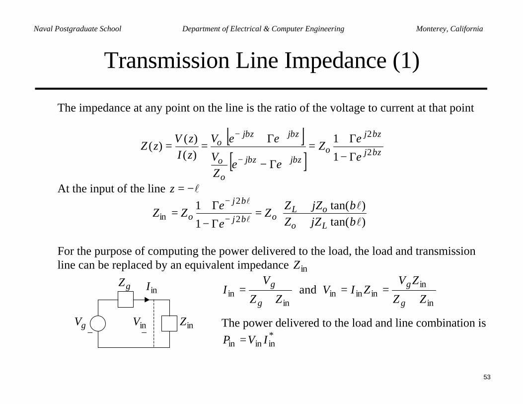
Transmission Line Impedance (1)
The impedance at any point on the line is the ratio of the voltage to current at that point
[ ][ ] zj
zj
ozjzj
o
o
zjzjo
e
eZ
eeZV
eeVzIzV
zZ β
β
ββ
ββ
2
2
1
1)()(
)(Γ−
Γ+=
Γ−
Γ+==
+−+
+−+
At the input of the line l−=z
++
=Γ−
Γ+= −
−
)tan()tan(
1
12
2
in ll
ll
ββ
β
β
Lo
oLoj
j
o jZZjZZ
Ze
eZZ
For the purpose of computing the power delivered to the load, the load and transmissionline can be replaced by an equivalent impedance inZ
gZ
gV inV
inI
+
−
+
−inZ
inin ZZ
VI
g
g
+= and
in
inininin ZZ
ZVZIV
g
g
+==
The power delivered to the load and line combination is*ininin IVP =
54
Naval Postgraduate School Department of Electrical & Computer Engineering Monterey, California
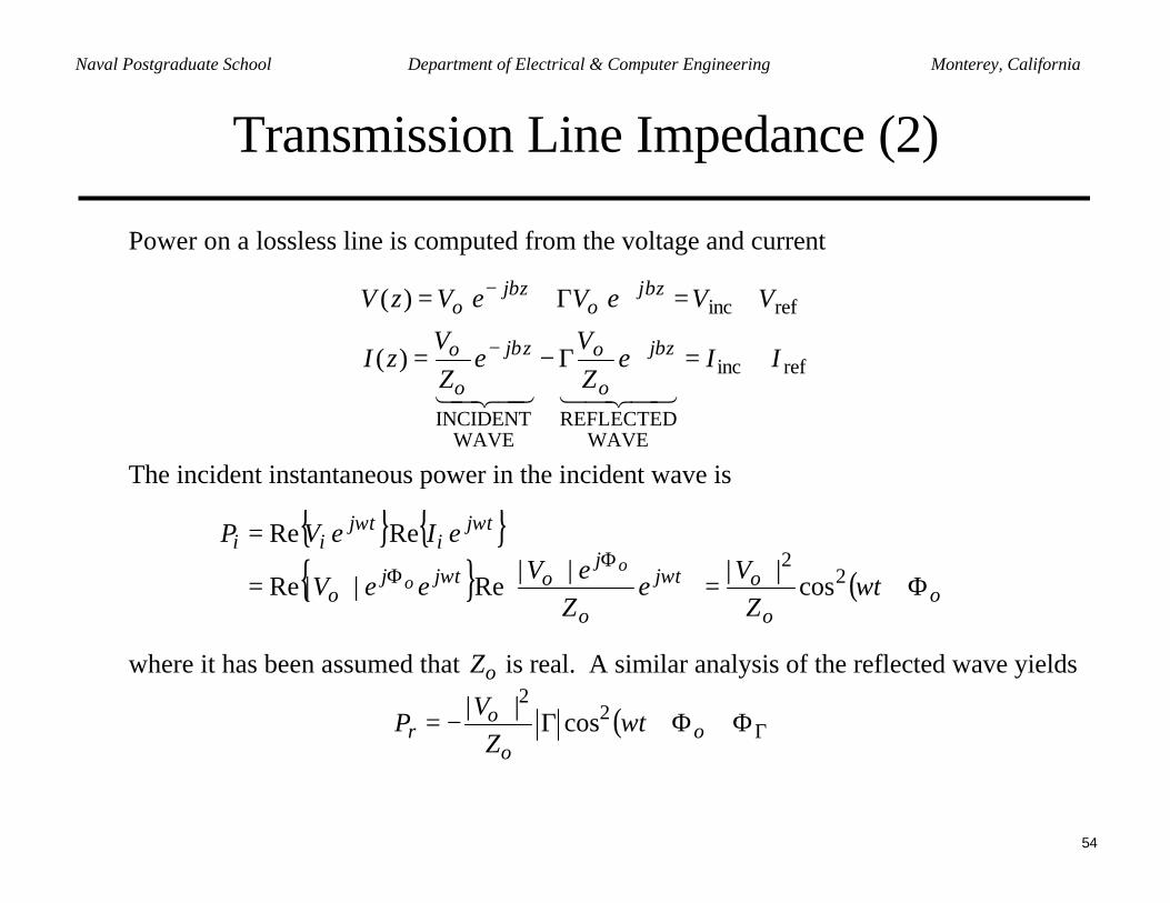
Transmission Line Impedance (2)
Power on a lossless line is computed from the voltage and current
refinc
WAVEREFLECTED
WAVEINCIDENT
refinc
)(
)(
IIeZV
eZV
zI
VVeVeVzV
zj
o
ozj
o
o
zjo
zjo
+=Γ−=
+=Γ+=
++
−+
++−+
4342143421ββ
ββ
The incident instantaneous power in the incident wave is
( )o
o
otj
o
jotjj
o
tji
tjii
tZ
Ve
ZeV
eeV
eIeVPo
o Φ+=
=
=+Φ+
Φ+ ωωω
ωω
22
cos||||
Re||Re
ReRe
where it has been assumed that oZ is real. A similar analysis of the reflected wave yields
( )Γ
+Φ+Φ+Γ−= o
o
or t
ZV
P ω22
cos||
55
Naval Postgraduate School Department of Electrical & Computer Engineering Monterey, California
Transmission Line Impedance (3)
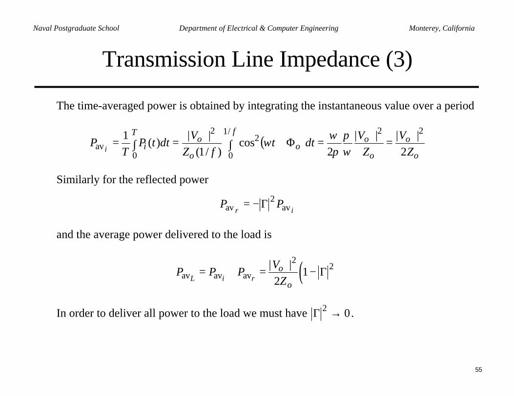
The time-averaged power is obtained by integrating the instantaneous value over a period
( )o
o
o
of
oo
oT
i ZV
ZV
dttfZ
VdttP
TP
i 2||||
2cos
)/1(||
)(1 22/1
0
22
0av
+++==∫ Φ+=∫=
ωπ
πω
ω
Similarly for the reflected power
irPP av
2av Γ−=
and the average power delivered to the load is
( )2
2av av av
| |1
2L i ro
o
VP P P
Z
+= + = − Γ
In order to deliver all power to the load we must have 02 →Γ .
56
Naval Postgraduate School Department of Electrical & Computer Engineering Monterey, California
Transmission Line Impedance (4)
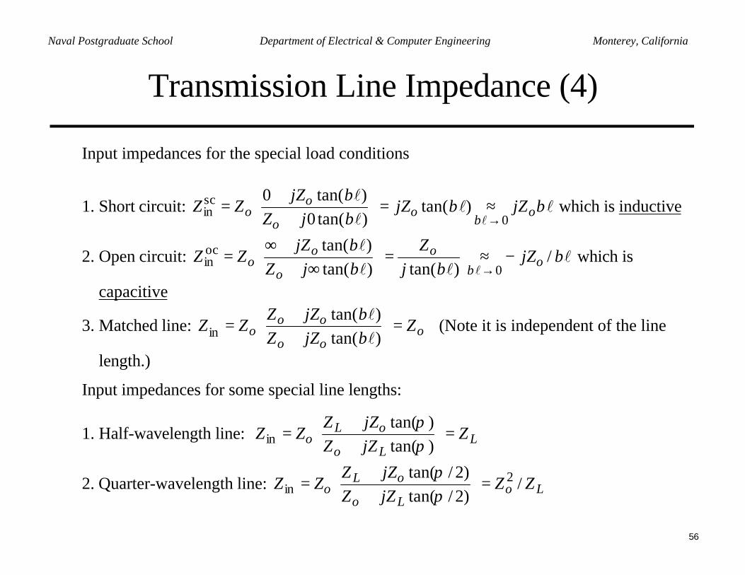
Input impedances for the special load conditions
1. Short circuit: llll
lββ
ββ
βoo
o
oo jZjZ
jZjZ
ZZ0
scin )tan(
)tan(0)tan(0
→≈=
+
+= which is inductive
2. Open circuit: llll
lβ
βββ
β/
)tan()tan()tan(
0
ocin o
o
o
oo jZ
jZ
jZjZ
ZZ −≈=
∞+
+∞=
→ which is
capacitive
3. Matched line: ooo
ooo Z
jZZjZZ
ZZ =
++
=)tan()tan(
in ll
ββ
(Note it is independent of the line
length.)
Input impedances for some special line lengths:
1. Half-wavelength line: LLo
oLo Z
jZZjZZ
ZZ =
++
=)tan()tan(
in ππ
2. Quarter-wavelength line: LoLo
oLo ZZ
jZZjZZ
ZZ /)2/tan()2/tan( 2
in =
++
=ππ
57
Naval Postgraduate School Department of Electrical & Computer Engineering Monterey, California
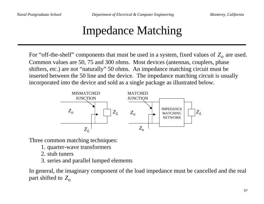
Impedance Matching
For “off-the-shelf” components that must be used in a system, fixed values of oZ are used.Common values are 50, 75 and 300 ohms. Most devices (antennas, couplers, phaseshifters, etc.) are not “naturally” 50 ohms. An impedance matching circuit must beinserted between the 50 line and the device. The impedance matching circuit is usuallyincorporated into the device and sold as a single package as illustrated below.
LZZo
LZ
MISMATCHEDJUNCTION
LZZo
Zo
MATCHEDJUNCTION
IMPEDANCEMATCHINGNETWORK
Three common matching techniques:1. quarter-wave transformers2. stub tuners3. series and parallel lumped elements
In general, the imaginary component of the load impedance must be cancelled and the realpart shifted to oZ
58
Naval Postgraduate School Department of Electrical & Computer Engineering Monterey, California
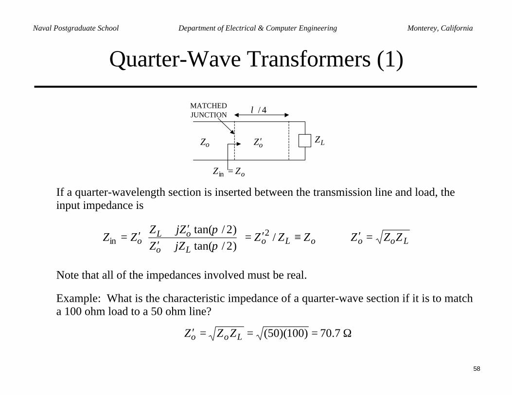
Quarter-Wave Transformers (1)
LZZo
oZZ =in
MATCHEDJUNCTION
oZ ′
4/λ
If a quarter-wavelength section is inserted between the transmission line and load, theinput impedance is
LoooLoLo
oLo ZZZZZZ
jZZZjZ
ZZ =′⇒≡′=
+′
′+′= /)2/tan()2/tan( 2
in ππ
Note that all of the impedances involved must be real.
Example: What is the characteristic impedance of a quarter-wave section if it is to matcha 100 ohm load to a 50 ohm line?
Ω===′ 7.70)100)(50(Loo ZZZ
59
Naval Postgraduate School Department of Electrical & Computer Engineering Monterey, California
Quarter-Wave Transformers (2)
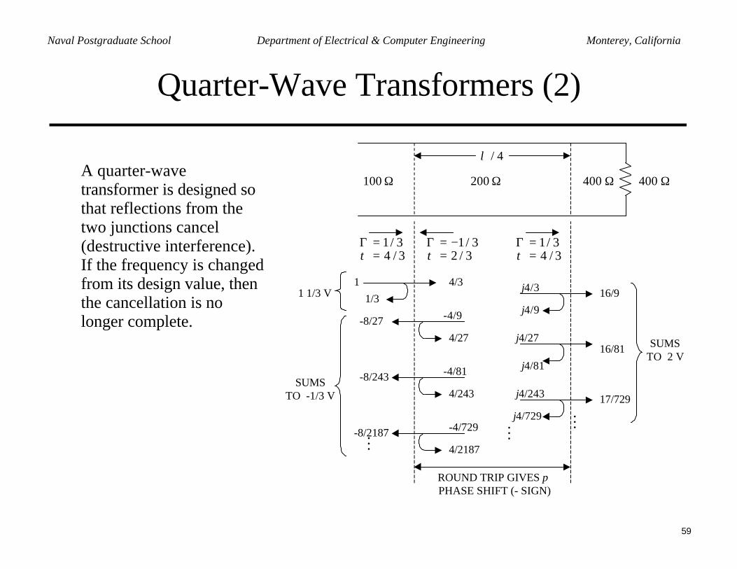
A quarter-wavetransformer is designed sothat reflections from thetwo junctions cancel(destructive interference).If the frequency is changedfrom its design value, thenthe cancellation is nolonger complete.
100 Ω 200 Ω 400 Ω 400 Ω
λ / 4
Γ = 1/ 3τ = 4 / 3
Γ = −1/ 3τ = 2 / 3
Γ = 1/ 3τ = 4 / 3
1 4/31/3
j4/3
j4/9-4/9
16/9
-8/27
-8/243
-8/2187
16/814/27 j4/27
-4/81
4/243
j4/81
j4/243 17/729
-4/729
4/2187
j4/729
1 1/3 V
SUMSTO -1/3 V
SUMSTO 2 V
ROUND TRIP GIVES π PHASE SHIFT (- SIGN)
M M M
60
Naval Postgraduate School Department of Electrical & Computer Engineering Monterey, California
Transmission Line Loss and Attenuation
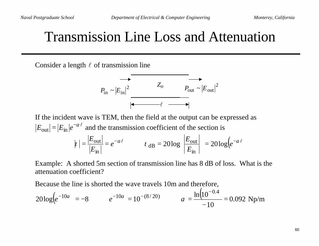
Consider a length l of transmission line
2inin ~ EP
Zo
l
2outout ~ EP
If the incident wave is TEM, then the field at the output can be expressed aslα−= eEE inout and the transmission coefficient of the section is
( )ll αα ττ −− =
=⇒== e
EE
eEE
log20log20in
outdB
in
out
Example: A shorted 5m section of transmission line has 8 dB of loss. What is theattenuation coefficient?
Because the line is shorted the wave travels 10m and therefore,
( ) ( )092.0
1010ln
108log204.0
)20/8(1010 =−
=⇒=⇒−=−
−−− ααα ee Np/m
61
Naval Postgraduate School Department of Electrical & Computer Engineering Monterey, California
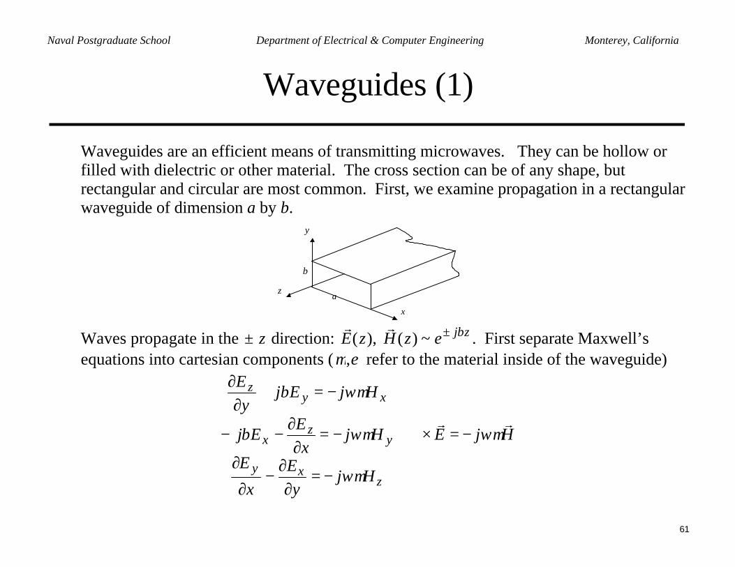
Waveguides (1)
Waveguides are an efficient means of transmitting microwaves. They can be hollow orfilled with dielectric or other material. The cross section can be of any shape, butrectangular and circular are most common. First, we examine propagation in a rectangularwaveguide of dimension a by b.
x
z
y
a
b
Waves propagate in the z± direction: zjezHzE β±~)(),(rr
. First separate Maxwell’sequations into cartesian components ( εµ, refer to the material inside of the waveguide)
HjE
Hjy
Ex
E
Hjx
EEj
HjEjy
E
zxy
yz
x
xyz
rrωµ
ωµ
ωµβ
ωµβ
−=×∇
−=∂
∂−
∂
∂
−=∂
∂−−
−=+∂
∂
62
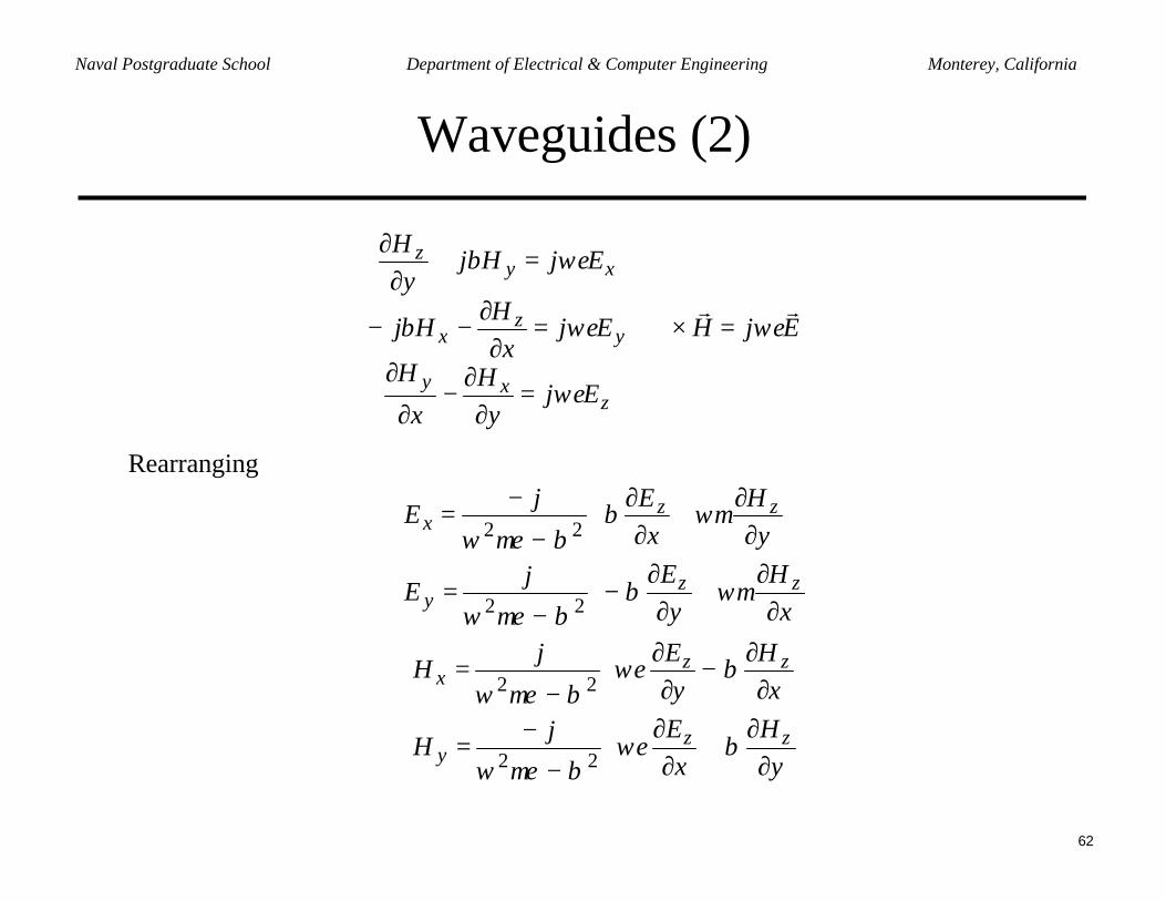
Naval Postgraduate School Department of Electrical & Computer Engineering Monterey, California
Waveguides (2)
EjH
Ejy
Hx
H
Ejx
HHj
EjHjy
H
zxy
yz
x
xyz
rrωε
ωε
ωεβ
ωεβ
=×∇
=∂
∂−
∂
∂
=∂
∂−−
=+∂
∂
Rearranging
∂
∂+
∂∂
−−
=
∂
∂+
∂∂
−
−=
xH
yEj
E
yH
xEj
E
zzy
zzx
ωµββµεω
ωµββµεω
22
22
∂
∂+
∂∂
−
−=
∂
∂−
∂∂
−=
yH
xEj
H
xH
yEj
H
zzy
zzx
βωεβµεω
βωεβµεω
22
22
63
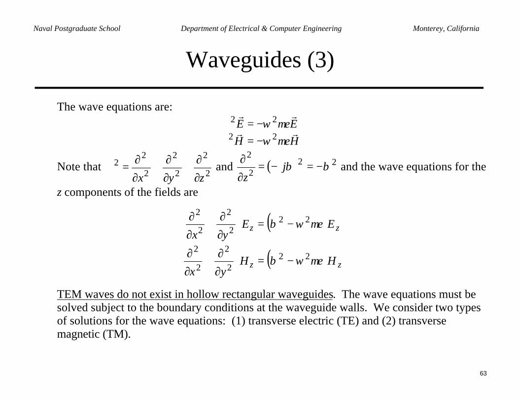
Naval Postgraduate School Department of Electrical & Computer Engineering Monterey, California
Waveguides (3)
The wave equations are:
HHEE rrrr
µεωµεω
22
22
−=∇−=∇
Note that 2
2
2
2
2
22
zyx ∂
∂+
∂
∂+
∂
∂=∇ and ( ) 22
2
2ββ −=−=
∂
∂j
z and the wave equations for the
z components of the fields are
( )
( ) zz
zz
HHyx
EEyx
µεωβ
µεωβ
222
2
2
2
222
2
2
2
−=
∂
∂+
∂
∂
−=
∂
∂+
∂
∂
TEM waves do not exist in hollow rectangular waveguides. The wave equations must besolved subject to the boundary conditions at the waveguide walls. We consider two typesof solutions for the wave equations: (1) transverse electric (TE) and (2) transversemagnetic (TM).
64
Naval Postgraduate School Department of Electrical & Computer Engineering Monterey, California
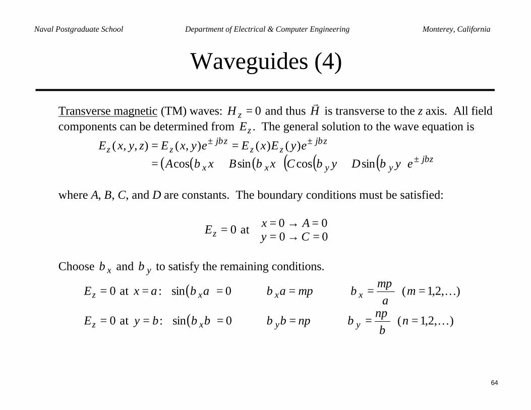
Waveguides (4)
Transverse magnetic (TM) waves: 0=zH and thus Hr
is transverse to the z axis. All fieldcomponents can be determined from zE . The general solution to the wave equation is
( ) ( )( ) ( ) ( )( ) zjyyxx
zjzz
zjzz
eyDyCxBxAeyExEeyxEzyxE
β
ββ
ββββ ±
±±
++===
sincossincos)()(),(),,(
where A, B, C, and D are constants. The boundary conditions must be satisfied:
0=zE at
=→==→=
0000
CyAx
Choose xβ and yβ to satisfy the remaining conditions.
0=zE at ax = : ( )a
mmaa xxx
πβπββ =⇒=⇒= 0sin ( …,2,1=m )
0=zE at by = : ( )b
nnbb yyx
πβπββ =⇒=⇒= 0sin ( …,2,1=n )
65
Naval Postgraduate School Department of Electrical & Computer Engineering Monterey, California
Waveguides (5)
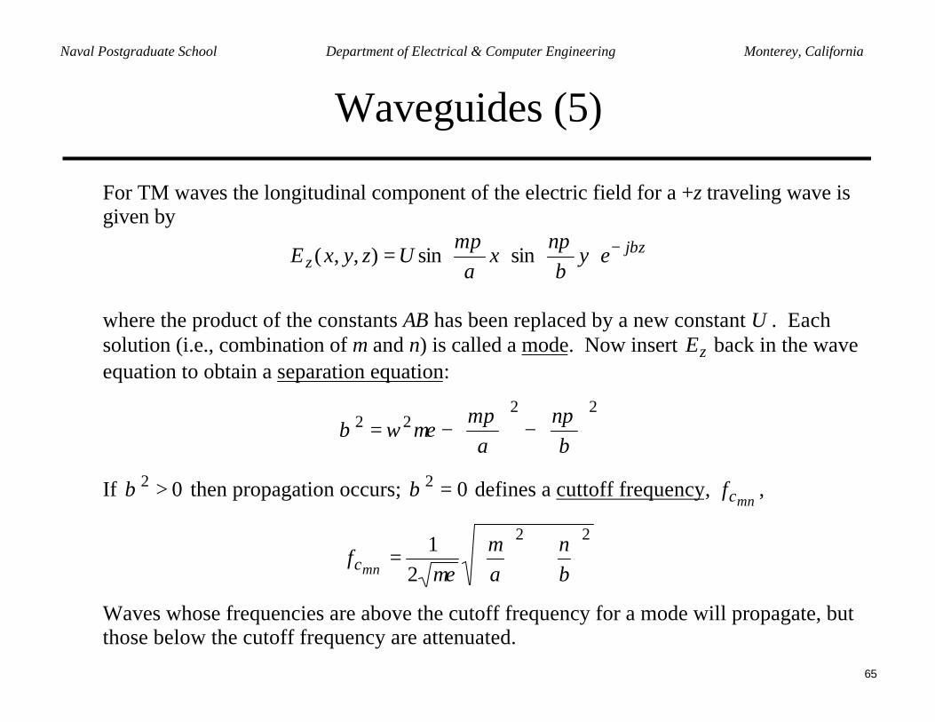
For TM waves the longitudinal component of the electric field for a +z traveling wave isgiven by
zjz ey
bn
xa
mUzyxE βππ −
= sinsin),,(
where the product of the constants AB has been replaced by a new constant U . Eachsolution (i.e., combination of m and n) is called a mode. Now insert zE back in the waveequation to obtain a separation equation:
2222
−
−=
bn
am ππ
µεωβ
If 02 >β then propagation occurs; 02 =β defines a cuttoff frequency, mncf ,
22
21
+
=
bn
am
fmnc µε
Waves whose frequencies are above the cutoff frequency for a mode will propagate, butthose below the cutoff frequency are attenuated.
66
Naval Postgraduate School Department of Electrical & Computer Engineering Monterey, California
Waveguides (6)
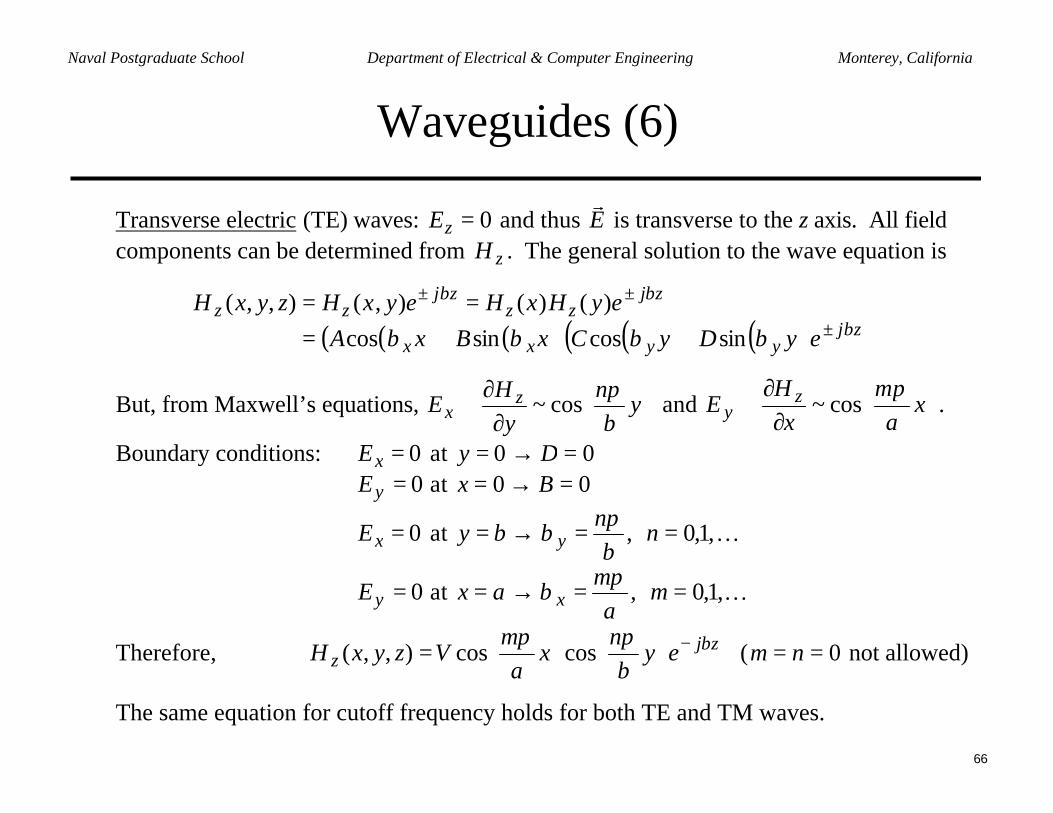
Transverse electric (TE) waves: 0=zE and thus Er
is transverse to the z axis. All fieldcomponents can be determined from zH . The general solution to the wave equation is
( ) ( )( ) ( ) ( )( ) zjyyxx
zjzz
zjzz
eyDyCxBxAeyHxHeyxHzyxH
β
ββ
ββββ ±
±±
++===
sincossincos)()(),(),,(
But, from Maxwell’s equations,
∂∂
∝ yb
ny
HE z
xπ
cos~ and
∂∂
∝ xa
mx
HE z
yπ
cos~ .
Boundary conditions: 0=xE at 00 =→= Dy0=yE at 00 =→= Bx
0=xE at b
nby y
πβ =→= , …,1,0=n
0=yE at a
max x
πβ =→= , …,1,0=m
Therefore, zjz ey
bn
xa
mVzyxH βππ −
= coscos),,( ( 0== nm not allowed)
The same equation for cutoff frequency holds for both TE and TM waves.
67
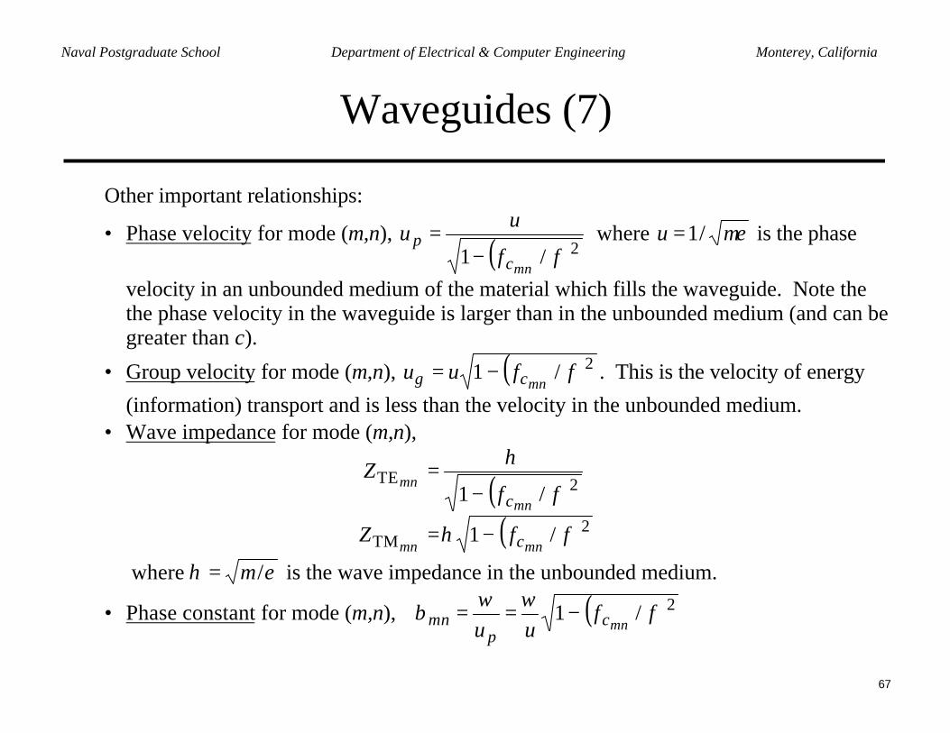
Naval Postgraduate School Department of Electrical & Computer Engineering Monterey, California
Waveguides (7)
Other important relationships:
• Phase velocity for mode (m,n), ( )2/1 ff
uu
mncp
−= where µε/1=u is the phase
velocity in an unbounded medium of the material which fills the waveguide. Note thethe phase velocity in the waveguide is larger than in the unbounded medium (and can begreater than c).
• Group velocity for mode (m,n), ( )2/1 ffuumncg −= . This is the velocity of energy
(information) transport and is less than the velocity in the unbounded medium.• Wave impedance for mode (m,n),
( )( )2TM
2TE
/1
/1
ffZ
ffZ
mnmn
mn
mn
c
c
−=
−=
η
η
where εµη /= is the wave impedance in the unbounded medium.
• Phase constant for mode (m,n), ( )2/1 ffuu mnc
pmn −==
ωωβ
68
Naval Postgraduate School Department of Electrical & Computer Engineering Monterey, California
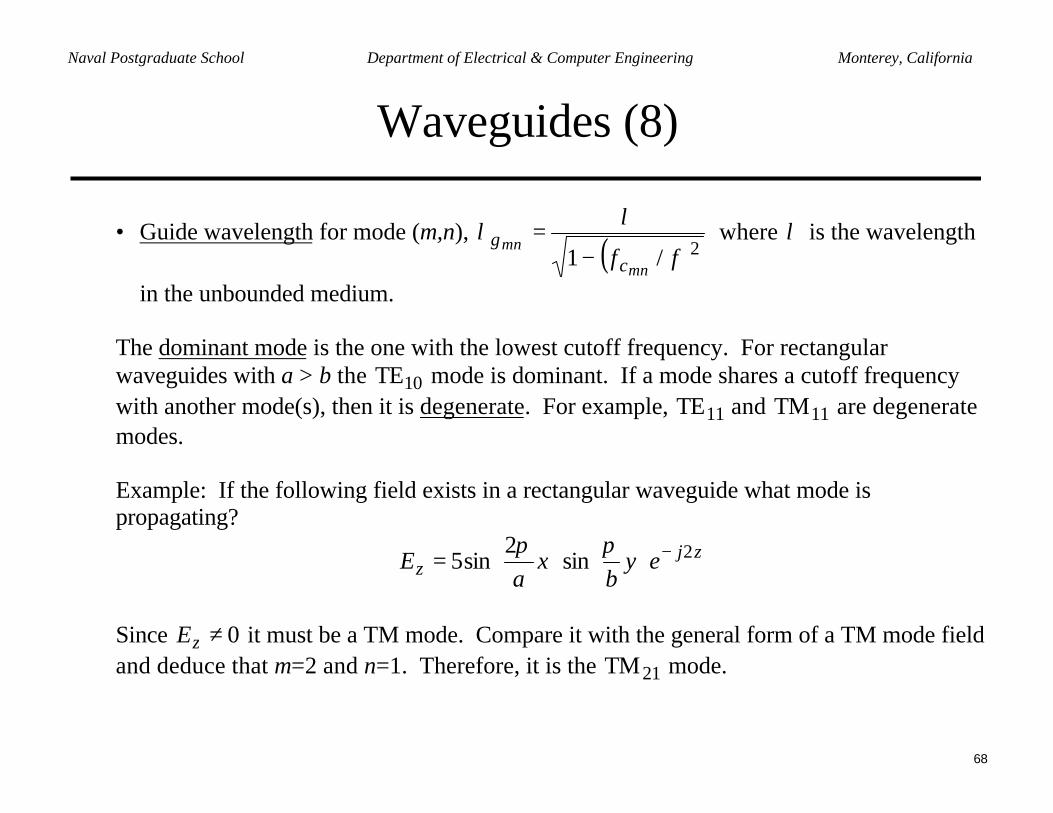
Waveguides (8)
• Guide wavelength for mode (m,n), ( )2/1 ff
mn
mnc
g−
=λ
λ where λ is the wavelength
in the unbounded medium.
The dominant mode is the one with the lowest cutoff frequency. For rectangularwaveguides with a > b the 10TE mode is dominant. If a mode shares a cutoff frequencywith another mode(s), then it is degenerate. For example, 11TE and 11TM are degeneratemodes.
Example: If the following field exists in a rectangular waveguide what mode ispropagating?
zjz ey
bx
aE 2sin
2sin5 −
=
ππ
Since 0≠zE it must be a TM mode. Compare it with the general form of a TM mode fieldand deduce that m=2 and n=1. Therefore, it is the 21TM mode.
69
Naval Postgraduate School Department of Electrical & Computer Engineering Monterey, California
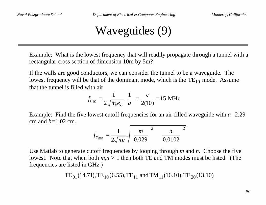
Waveguides (9)
Example: What is the lowest frequency that will readily propagate through a tunnel with arectangular cross section of dimension 10m by 5m?
If the walls are good conductors, we can consider the tunnel to be a waveguide. Thelowest frequency will be that of the dominant mode, which is the 10TE mode. Assumethat the tunnel is filled with air
15)10(2
12
110
==
=
ca
foo
c εµ MHz
Example: Find the five lowest cutoff frequencies for an air-filled waveguide with a=2.29cm and b=1.02 cm.
22
0102.0029.021
+
=
nmf
mnc µε
Use Matlab to generate cutoff frequencies by looping through m and n. Choose the fivelowest. Note that when both m,n > 1 then both TE and TM modes must be listed. (Thefrequencies are listed in GHz.)
)10.13(TE),10.16(TM and TE),55.6(TE),71.14(TE 2011111001
70
Naval Postgraduate School Department of Electrical & Computer Engineering Monterey, California
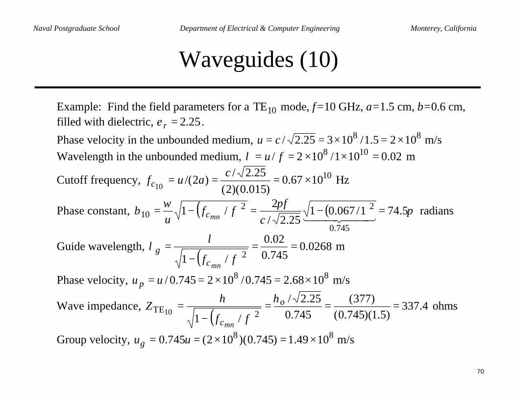
Waveguides (10)
Example: Find the field parameters for a 10TE mode, f=10 GHz, a=1.5 cm, b=0.6 cm,filled with dielectric, 25.2=rε .
Phase velocity in the unbounded medium, 88 1025.1/10325.2/ ×=×== cu m/sWavelength in the unbounded medium, 02.0101/102/ 108 =××== fuλ m
Cutoff frequency, 101067.0)015.0)(2(
25.2/)2/(
10×===
caufc Hz
Phase constant, ( ) ( ) ππω
β 5.741/067.0125.2/
2/1
745.0
2210 =−=−= 44 344 21c
fff
u mnc radians
Guide wavelength, ( )
0268.0745.002.0
/1 2==
−=
ffmnc
gλ
λ m
Phase velocity, 88 1068.2745.0/102745.0/ ×=×== uu p m/s
Wave impedance, ( )
4.337)5.1)(745.0(
)377(745.0
25.2/
/1 2TE10===
−= o
c ffZ
mn
ηη ohms
Group velocity, 88 1049.1)745.0)(102(745.0 ×=×== uug m/s
71
Naval Postgraduate School Department of Electrical & Computer Engineering Monterey, California
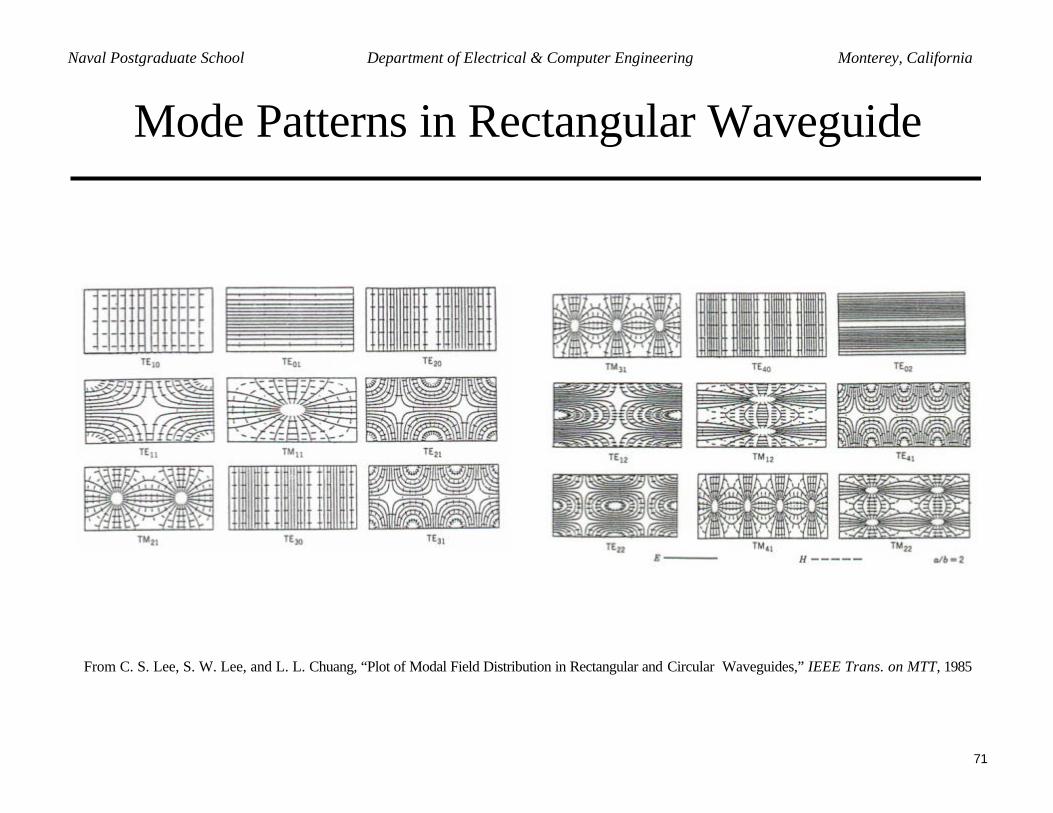
Mode Patterns in Rectangular Waveguide
From C. S. Lee, S. W. Lee, and L. L. Chuang, “Plot of Modal Field Distribution in Rectangular and Circular Waveguides,” IEEE Trans. on MTT, 1985
72
Naval Postgraduate School Department of Electrical & Computer Engineering Monterey, California
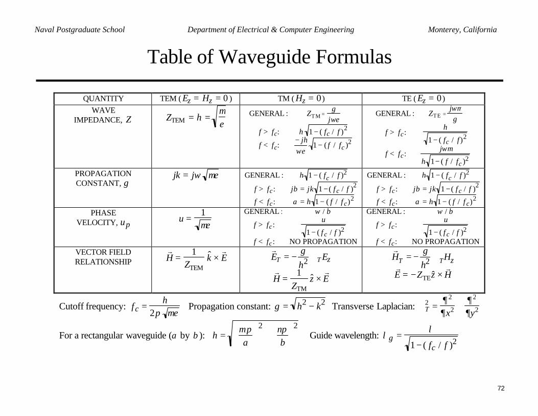
Table of Waveguide Formulas
QUANTITY TEM ( Ez = Hz = 0 ) TM ( Hz = 0 ) TE ( Ez = 0 )WAVE
IMPEDANCE, Z ZTEM = η =µε
GENERAL : ZTM =γ
jωε
f > fc: η 1 − ( fc / f )2
f < fc:− jhωε
1 − ( f / fc )2
GENERAL : ZTE =jωµγ
f > fc:η
1 − ( fc / f )2
f < fc:jωµ
h 1− ( f / fc )2
PROPAGATIONCONSTANT, γ
jk = jω µε GENERAL : h 1 − ( fc / f )2
f > fc: jβ = jk 1 − ( f c / f )2
f < fc: α = h 1 − ( f / f c)2
GENERAL : h 1 − ( fc / f )2
f > fc: jβ = jk 1 − ( f c / f )2
f < fc: α = h 1 − ( f / f c)2
PHASEVELOCITY, up
u =1µε
GENERAL : ω / β
f > fc:u
1 − ( f c / f )2
f < fc: NO PROPAGATION
GENERAL : ω / β
f > fc:u
1 − ( f c / f )2
f < fc: NO PROPAGATIONVECTOR FIELDRELATIONSHIP
r H =
1ZTEM
ˆ k ×r E
r E T = −
γh2 ∇T Ez
r H =
1ZTM
ˆ z ×r E
r H T = −
γh2 ∇THzr
E = −ZTEˆ z ×r H
Cutoff frequency: fc =h
2π µε Propagation constant: γ = h2 − k2 Transverse Laplacian: ∇T
2 =∂ 2
∂x2 +∂ 2
∂y2
For a rectangular waveguide (a by b ): h =mπa
2+
nπb
2 Guide wavelength: λg =
λ
1 − ( fc / f )2
73
Naval Postgraduate School Department of Electrical & Computer Engineering Monterey, California
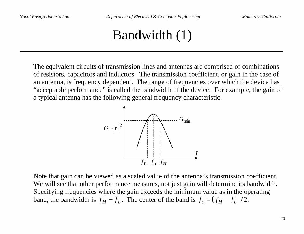
Bandwidth (1)
The equivalent circuits of transmission lines and antennas are comprised of combinationsof resistors, capacitors and inductors. The transmission coefficient, or gain in the case ofan antenna, is frequency dependent. The range of frequencies over which the device has“acceptable performance” is called the bandwidth of the device. For example, the gain ofa typical antenna has the following general frequency characteristic:
2~ τG
f
of HfLf
minG
Note that gain can be viewed as a scaled value of the antenna’s transmission coefficient.We will see that other performance measures, not just gain will determine its bandwidth.Specifying frequencies where the gain exceeds the minimum value as in the operatingband, the bandwidth is LH ff − . The center of the band is ( ) 2/LHo fff += .
74
Naval Postgraduate School Department of Electrical & Computer Engineering Monterey, California
Bandwidth (2)
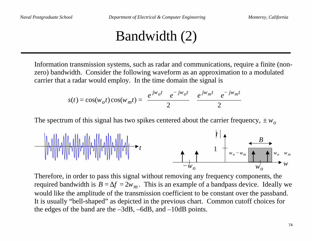
Information transmission systems, such as radar and communications, require a finite (non-zero) bandwidth. Consider the following waveform as an approximation to a modulatedcarrier that a radar would employ. In the time domain the signal is
+
+==
−−
22)cos()cos()(
tjtjtjtj
mommoo eeee
tttsωωωω
ωω
The spectrum of this signal has two spikes centered about the carrier frequency, oω±
t
ωoω
mo ωω +
oω−
mo ωω −
Bτ
1
Therefore, in order to pass this signal without removing any frequency components, therequired bandwidth is mfB ω2=∆= . This is an example of a bandpass device. Ideally wewould like the amplitude of the transmission coefficient to be constant over the passband.It is usually “bell-shaped” as depicted in the previous chart. Common cutoff choices forthe edges of the band are the –3dB, –6dB, and –10dB points.
75
Naval Postgraduate School Department of Electrical & Computer Engineering Monterey, California
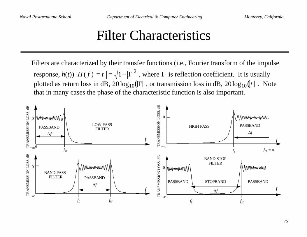
Filter Characteristics
Filters are characterized by their transfer functions (i.e., Fourier transform of the impulse
response, h(t)) 21)( Γ−== τfH , where Γ is reflection coefficient. It is usually plotted as return loss in dB, 20 log10 Γ( ), or transmission loss in dB, 20 log10 τ( ). Note that in many cases the phase of the characteristic function is also important.
PASSBAND
fH
∆ f
0
f
LOW PASS FILTER
PASSBAND
fL fH
∆ff
BAND PASS FILTER
−∞TR
AN
SMIS
SIO
N L
OSS
, dB
0
−∞TR
AN
SMIS
SIO
N L
OSS
, dB
0
fH
PASSBAND
∆ff
PASSBAND
BAND STOP FILTER
STOPBAND
fL
fL fH = ∞
PASSBAND
∆f
f
HIGH PASS
−∞TR
AN
SMIS
SIO
N L
OSS
, dB
0
−∞TR
AN
SMIS
SIO
N L
OSS
, dB
0
76
Naval Postgraduate School Department of Electrical & Computer Engineering Monterey, California
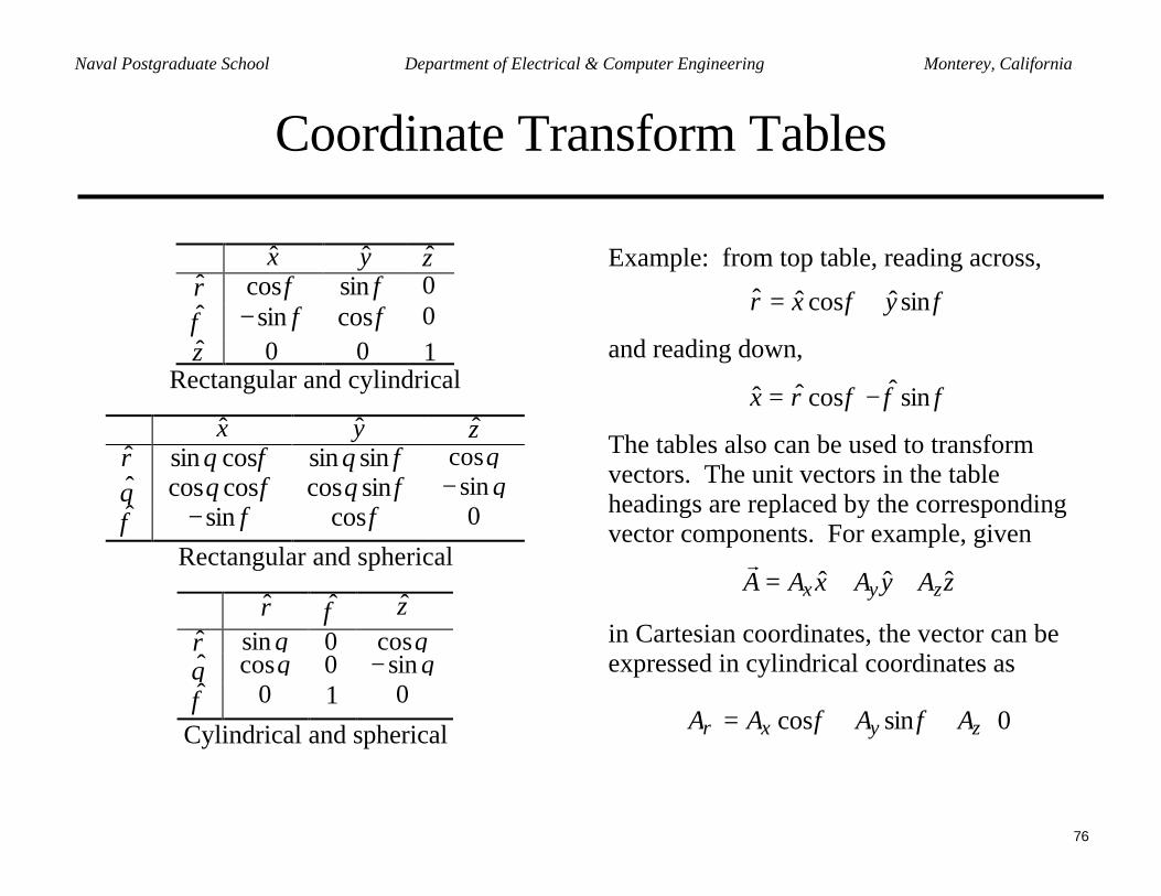
Coordinate Transform Tables
ˆ x ˆ y ˆ z ˆ ρ cosφ sin φ 0ˆ φ −sin φ cosφ 0ˆ z 0 0 1
Rectangular and cylindrical
ˆ x ˆ y ˆ z ˆ r sin θ cosφ sin θ sin φ cosθˆ θ cosθ cosφ cosθ sinφ − sin θˆ φ −sin φ cosφ 0
Rectangular and spherical
ˆ ρ ˆ φ ˆ z ˆ r sin θ 0 cosθˆ θ cosθ 0 − sin θˆ φ 0 1 0
Cylindrical and spherical
Example: from top table, reading across,
ˆ ρ = ˆ x cosφ + ˆ y sinφ
and reading down,
ˆ x = ˆ ρ cosφ − ˆ φ sin φ
The tables also can be used to transformvectors. The unit vectors in the tableheadings are replaced by the correspondingvector components. For example, given
r A = Ax ˆ x + Ay ˆ y + Az ˆ z
in Cartesian coordinates, the vector can beexpressed in cylindrical coordinates as
Aρ = Ax cosφ + Ay sinφ + Az ⋅ 0
77
Naval Postgraduate School Department of Electrical & Computer Engineering Monterey, California
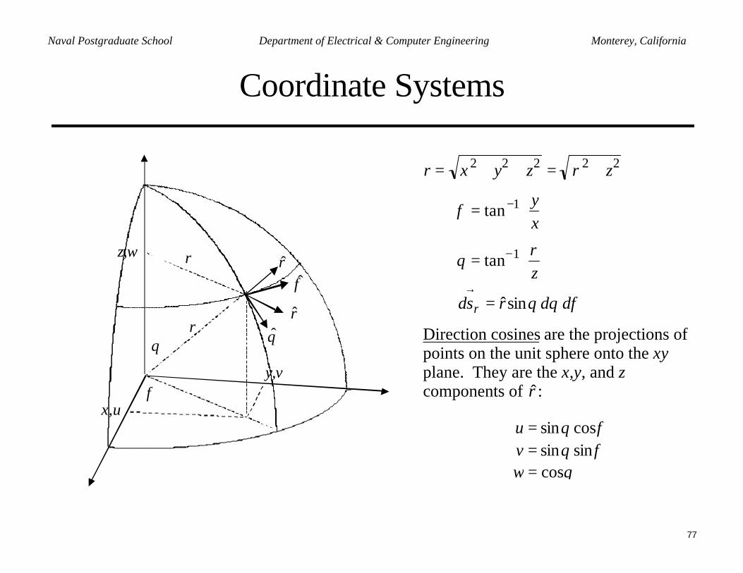
Coordinate Systems
x,u
y,v
z,w
φ
θ
ρ
rˆ ρ
ˆ r
ˆ θ
ˆ φ
r = x 2 + y2 + z2 = ρ2 + z2
φ = tan−1 yx
θ = tan−1 ρz
φθθ ddrdsr sinˆ=→
Direction cosines are the projections ofpoints on the unit sphere onto the xyplane. They are the x,y, and zcomponents of r :
θφθφθ
cossinsincossin
===
wvu
78
Naval Postgraduate School Department of Electrical & Computer Engineering Monterey, California
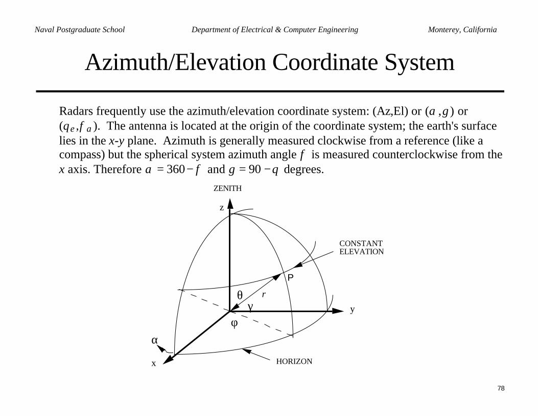
Azimuth/Elevation Coordinate System
Radars frequently use the azimuth/elevation coordinate system: (Az,El) or (α ,γ ) or( ae φθ , ). The antenna is located at the origin of the coordinate system; the earth's surfacelies in the x-y plane. Azimuth is generally measured clockwise from a reference (like acompass) but the spherical system azimuth angle φ is measured counterclockwise from thex axis. Therefore α = 360− φ and γ = 90 −θ degrees.
CONSTANT ELEVATION
x
y
z
θ
φγ
ZENITH
HORIZON
P
α
r
79
Naval Postgraduate School Department of Electrical & Computer Engineering Monterey, California
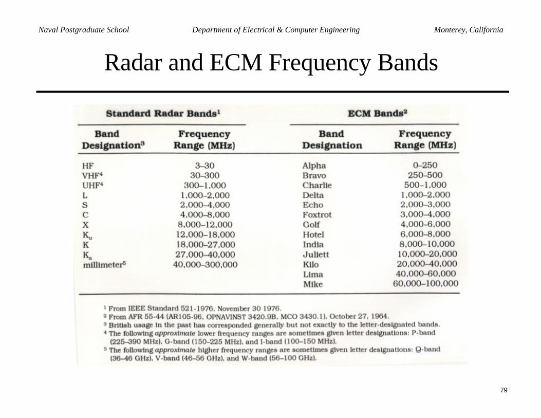
Radar and ECM Frequency Bands
80
Naval Postgraduate School Department of Electrical & Computer Engineering Monterey, California
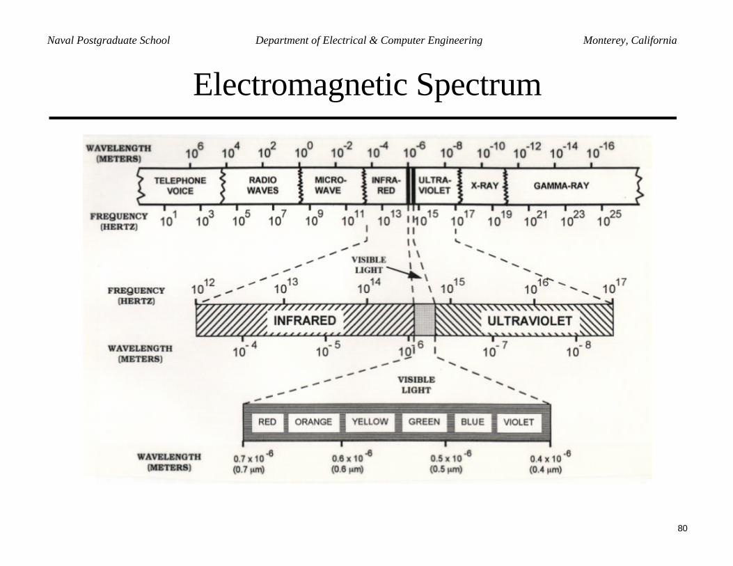
Electromagnetic Spectrum
81
Naval Postgraduate School Department of Electrical & Computer Engineering Monterey, California
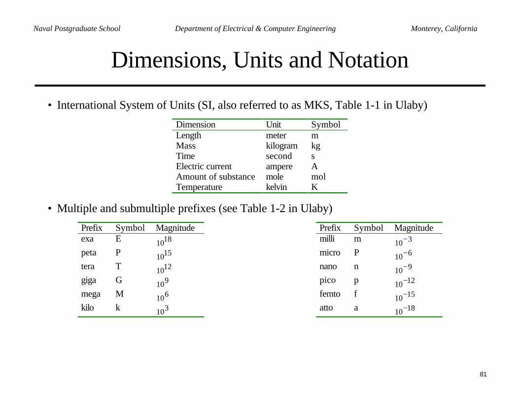
Dimensions, Units and Notation
• International System of Units (SI, also referred to as MKS, Table 1-1 in Ulaby)
Dimension Unit SymbolLength meter mMass kilogram kgTime second sElectric current ampere AAmount of substance mole molTemperature kelvin K
• Multiple and submultiple prefixes (see Table 1-2 in Ulaby)
Prefix Symbol Magnitudeexa E 1810peta P 1510tera T 1210giga G 910mega M 610kilo k 310
Prefix Symbol Magnitudemilli m 310−
micro P 610−
nano n 910−
pico p 1210−
femto f 1510−
atto a 1810−
82
Naval Postgraduate School Department of Electrical & Computer Engineering Monterey, California
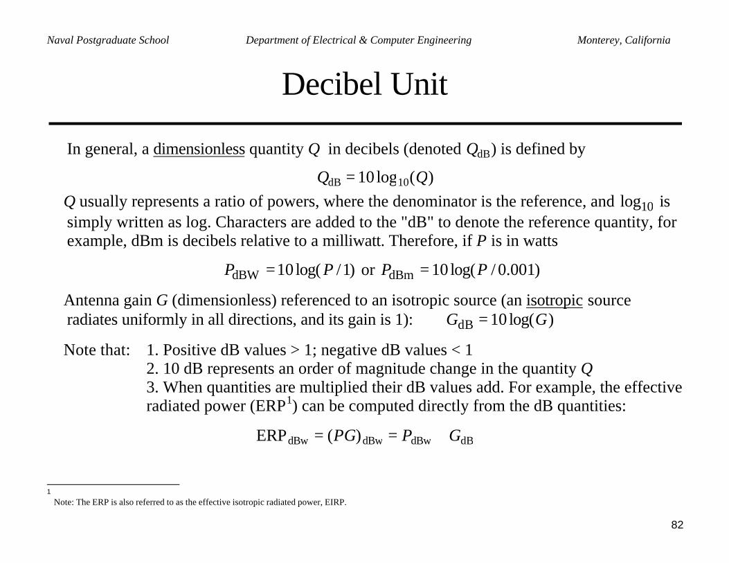
Decibel Unit
In general, a dimensionless quantity Q in decibels (denoted QdB) is defined by
QdB = 10 log10(Q)Q usually represents a ratio of powers, where the denominator is the reference, and 10log issimply written as log. Characters are added to the "dB" to denote the reference quantity, forexample, dBm is decibels relative to a milliwatt. Therefore, if P is in watts
)1/log(10dBW PP = or )001.0/log(10dBm PP =
Antenna gain G (dimensionless) referenced to an isotropic source (an isotropic sourceradiates uniformly in all directions, and its gain is 1): )log(10dB GG =
Note that: 1. Positive dB values > 1; negative dB values < 12. 10 dB represents an order of magnitude change in the quantity Q3. When quantities are multiplied their dB values add. For example, the effectiveradiated power (ERP1) can be computed directly from the dB quantities:
ERPdBw = (PG)dBw = PdBw + GdB
1
Note: The ERP is also referred to as the effective isotropic radiated power, EIRP.
83
Naval Postgraduate School Department of Electrical & Computer Engineering Monterey, California
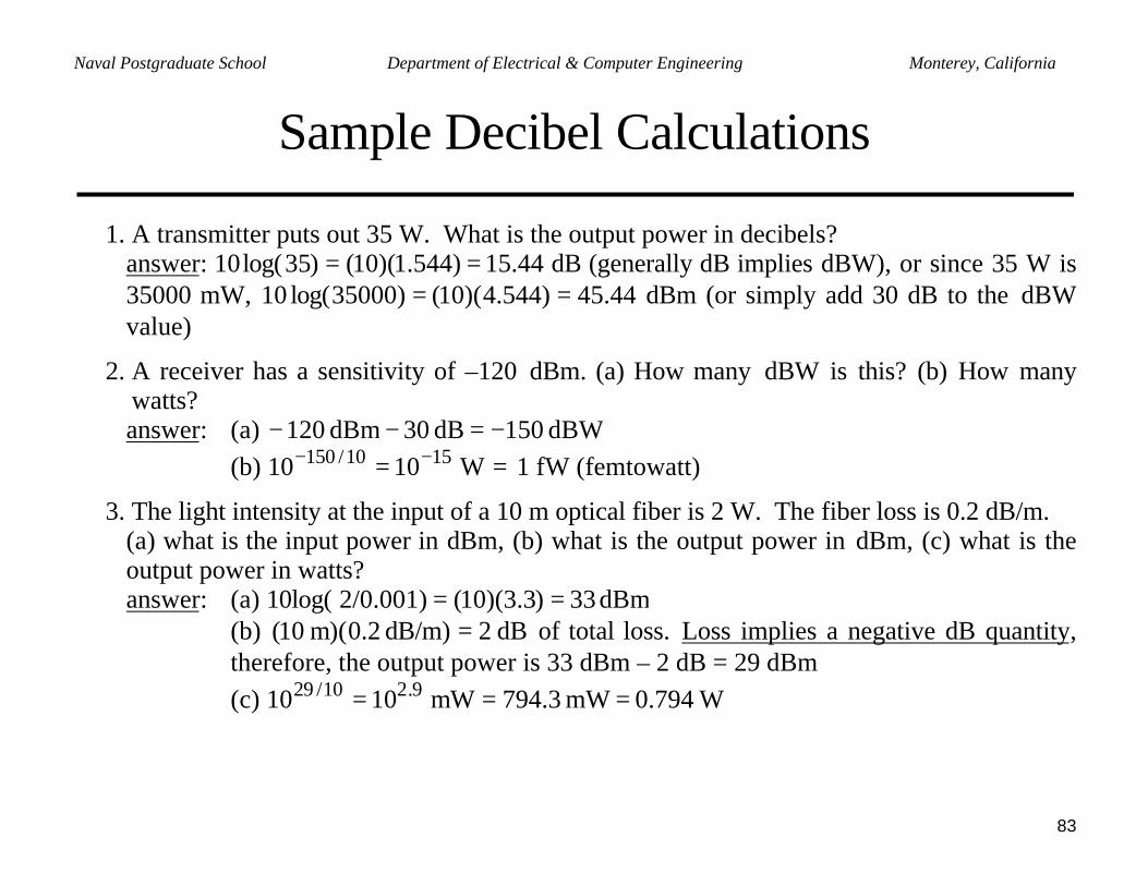
Sample Decibel Calculations
1. A transmitter puts out 35 W. What is the output power in decibels?answer: 44.15)544.1)(10()35log(10 == dB (generally dB implies dBW), or since 35 W is35000 mW, 44.45)544.4)(10()35000log(10 == dBm (or simply add 30 dB to the dBWvalue)
2. A receiver has a sensitivity of –120 dBm. (a) How many dBW is this? (b) How manywatts?answer: (a) dBW 150dB 30dBm 120 −=−−
(b) == −− W1010 1510/150 1 fW (femtowatt)
3. The light intensity at the input of a 10 m optical fiber is 2 W. The fiber loss is 0.2 dB/m.(a) what is the input power in dBm, (b) what is the output power in dBm, (c) what is theoutput power in watts?answer: (a) dBm 33)3.3)(10(2/0.001) 10log( ==
(b) dB 2dB/m) 2.0(m) 10( = of total loss. Loss implies a negative dB quantity,therefore, the output power is 33 dBm – 2 dB = 29 dBm(c) W0.794 mW 3.794mW 1010 9.210/29 ===