PI and PID Parameters from IMC Designs - BGU courses/Chapter 6... · PI and PID Parameters from IMC...

113

C H A P T E R 6

PI and PID Parameters from IMC Designs

Objectives of the Chapter

• Provide methods for approximating most IMC controllers with I, PI, or PID controllers. • Provide methods for approximating all other IMC controllers with PI or PID controllers

cascaded with first-order or second-order lags. Prerequisite Reading Chapter 3, “One-Degree of Freedom Internal Model Control” Chapter 4, “Two-Degree of Freedom Internal Model Control” Appendix A.3, “P, PI, and PID Controller Transfer Functions”

114 PI and PID Parameters from IMC Designs Chapter 6

6.1 INTRODUCTION

While IMC controller implementations are becoming more popular (see Chapter 5), the standard industrial controllers remain the proportional (P), proportional plus integral (PI), and the proportional plus integral and derivative (PID) controllers. Morari and Zafiriou (1989) and Rivera et al. (1986) show how to approximate the IMC controller for a limited class of processes with PI and PID controllers. To obtain a PID controller for the industrially important first-order lag and dead time process model, they approximate the dead time with a low-order Padé approximation. Because their approximations are surprisingly good, they conclude that there is relatively little to be gained in dynamic response by implementing the IMC controller rather than the PI or PID approximation.

While motivated by Morari’s work (Morari, 1989), this chapter presents a more general, yet conceptually simple, approach to approximating IMC controllers with I, PI or PID controllers using Maclaurin series approximations. The PID parameters so obtained all depend on the IMC filter time constant. As the filter time constant gets larger, the PID controller goes smoothly into a PI and a floating integral controller, just as intuition says it should. Since our IMC design methods always result in an offset-free control system, our simple feedback approximations always have an integrating action, and one never obtains a simple proportional controller (which always leads to offset for non-integrating processes).

This chapter assumes that the IMC filter time constant is known a priori either from considerations of process uncertainty as discussed in Chapter 7, or from consideration of noise amplification in the case of a perfect model as discussed in Chapter 3. However, the filter time constant that provides the desired maximum noise amplification for the IMC system often yields a PID controller that results in excessive overshoot to a step setpoint change. We have found that increasing the filter time constant always reduces the overshoot to an acceptable level. With the aid of IMCTUNE two or three trials usually provide a filter time constant that yields the desired overshoot. We generally take a 10% overshoot to a step setpoint change for a perfect process model to be a good approximation of the IMC closed loop response.

The approximation methods of this chapter provide analytical expressions for the dependence of controller gain, integral and derivative time constants model parameters, and the filter time constant for simple, but industrially important, process models such as a first-order lag plus dead time. In general, however, the simplest method for obtaining the PID parameters associated with any IMC design is via a computer program such as IMCTUNE that carries out the necessary calculations. The algorithms used in this program are described in sections 3 and 4 of this chapter. The inputs required by IMCTUNE to compute PID parameters are the process model, the portion of the model to be inverted by the controller, and the IMC controller filter time constant.

In the following section we review the time domain and Laplace transform representations of a common form of PID controller that is implemented in IMCTUNE. There is a more extensive discussion of the various types of controllers in Appendix A.3, and readers not familiar with the different types of controllers are urged to review this appendix.

6.3 1DF PID Parameters from 1DF IMC 115

6.2 THE PID CONTROLLER

The form of the PID controller that we will use in this chapter is given by

)()1

11()( ses + ταsτ +

sτ + = Ksu

D

D

Ic (6.1)

where α is a constant that is usually fixed between .05 and .2, depending on the manufacturer, to limit its high frequency gain to between 5 and 20 times its proportional gain K. Recall that in Chapter 3 on IMC controller design for perfect models, we adopted the same high frequency gain limitation for the IMC controller as is used for the PID controllers. A time domain implementation of the PID controller given by Eq. (6.1) can be expressed in terms of the error between the setpoint and measured process output, e(t), as follows

( )))()(()()()( 11 tetedtte + te = Ktu Lc I−+∫ ατ , (6.2)

Where eL(t) is a filtered version of e(t), given by

).()()( t = et + etedtdατ LLD (6.3)

The PID controller implemented in IMCTUNE is that given by Eq. (6.1) and its time domain representation given by Eq. (6.2).

The next section shows how to use IMC controller designs to find the PID gain and integral and derivative time constants that give IMC-like closed-loop responses.

6.3 1DF PID PARAMETERS FROM 1DF IMC

6.3.1 1DF PID Parameters for General Process Models

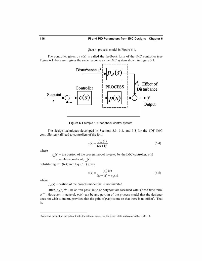
As shown in Section 3.2, the IMC structure reduces to the classical feedback structure of Figure 6.1, with the feedback form of the IMC controller, c(s), given by Eq. (3.1), which is repeated below.

,)()(~1

)()(sqsp

sqsc−

=

where

q(s) = 1DF IMC controller in Figure 6.1,


)(~ sp = process model in Figure 6.1.

The controller given by c(s) is called the feedback form of the IMC controller (see Figure 6.1) because it gives the same response as the IMC system shown in Figure 3.1.

c(s) p(s)Controller PROCESS

Disturbance d

de

Setpointr

Outputy

Effect ofDisturbance

−

pd (s)

c(s) p(s)Controller PROCESS

Disturbance d

de

Setpointr

Outputy



−

pd (s)

Figure 6.1 Simple 1DF feedback control system.

The design techniques developed in Sections 3.3, 3.4, and 3.5 for the 1DF IMC controller q(s) all lead to controllers of the form

rm

ssp

sq)1()(

)(1

+=

−

ε (6.4)

where p

m(s) = the portion of the process model inverted by the IMC controller, q(s)

r = relative order of pm(s).

Substituting Eq. (6.4) into Eq. (3.1) gives

)()1(

)()(

1

spssp

scA

rm

−+=

−

ε (6.5)

where pA(s) = portion of the process model that is not inverted.

Often, pA(s) will be an “all pass” ratio of polynomials cascaded with a dead time term, Tse− . However, in general, pA(s) can be any portion of the process model that the designer

does not wish to invert, provided that the gain of pA(s) is one so that there is no offset1. That is,

1 No offset means that the output tracks the setpoint exactly in the steady state and requires that pA(0) =1.


)()()(~ sps p sp Am≡ ; 1.)0( = pA (6.6)

Because pA(0) is 1, the denominator of Eq. (6.5) has zero at the origin, and c(s) can be re-written as

),(1)( sfs

sc ≡ (6.7)

where

.))()1((

)()(

1

sprεs

sspsf

A

m

−+≡

−

Expanding f (s) in a Maclaurin series in s gives

),22

)0()0()0((1c ...sfsffs

(s) +′′

+′+= (6.8)

...)11( +++= ss

K DI

c ττ

(6.9)

where

)0(fKc ′= ; )0()0( /ffIτ ′= ; ).0(2/)0( ffD ′′′=τ (6.10)

In order to evaluate the PID controller given by Eq. (6.10), we let

./))()1(()( sspssD Ar −+≡ ε (6.11a)

Then, by Maclaurin series expansion, we get

),0()0( AprD ′−= ε (6.11b)

,2/))0()1(()0( 2AprrD ′′−−=′ ε (6.11c)

.3/))0()2)(1(()0( 3AprrrD ′′′−−−=′′ ε (6.11d)

Using Eq. (6.11), the function )(sf and its first and second derivatives, all evaluated at the origin, are given by

,)0(

1)0(DK

fp

= (6.12a)

,))0((

))0()0()0(()0( 2DK

DKDpf

p

pm ′+′−=′ (6.12b)


,)0()0(2

)0()0()0()0()0()0(2)0()0(

)0()0(

′+

′+′′′+′′+′′

′=′′ff

DKDpDKDpDp

ffpm

pmm (6.12c)

where

Kp ≡ pm(0).

Equations (6.10) and (6.12) together can be used to obtain the controller gain and integral and derivative time constants as analytical functions of the process model and IMC controller parameters, including the IMC filter time constant. The PID parameters for a first-order lag dead time process are given below, and derived in the following subsection.

6.3.2 1DF PID Parameters for a First-Order Lag Plus Dead time Model

The process model is

)1(

)(+

=−

seK

spTs

p

τ (6.13)

The 1DF PID parameters for the model in Eq. (6.13) are given in Eq. (6.14). The derivation of these parameters from Equations (6.10) and (6.12) follows in Section 6.3.3.

)( T2

T 2

I ++=

εττ ;

)( TKK

p

Ic +

=ετ ;

)(2

)3

1(2

T

TTI

D +

−=

εττ (6.14)

Notice that, as one might expect, all the above PID parameters depend on the filter time constant. Further, the gain and derivative time constants go to zero as the filter time constant gets large. The integral time constant, on the other hand, approaches the model time constant.

6.3.3 Derivation of the 1DF PID Parameters of Eq. (6.14) for a First-Order Lag Plus Dead time Model

Following the IMC controller design procedures in Chapter 3, we select

)1(

)(+

≡sK

sp pm τ

TsA esp −≡)( (6.15a)

Therefore,


22)0(;)0(;)0( ττ pmpmpm KpKpKp =′′−=′= (6.15b)

32 )0(;)0(;)0(;1)0( TpTpTpp AAAA −=′′′=′′−=′= (6.15c)

Evaluating Equations (6.11b), (6.11c), and (6.11d) using Eq. (6.15c) and the fact that the relative order of the transfer function in Eq. (6.13) is one (i.e. r = 1) gives

.)0(;2/)0(;)0( 3/32 TDTDTD =′′′−=′+= ε (6.15d)

Substituting the above into Eq. (6.12) gives

,)(

1)0(TK

fp +

=ε

(6.15e)

,)(2

)()0( 2

2

TK

TTf

p +

++=′

ε

ετ (6.15f)

.2/)(

3/)(22)0()0( 2

322

+++++

+′=′′TKTK

TKTKTKff

pp

pppI ετ

τεττ (6.15g)

Finally, after some simplification, we get Eq. (6.14), which is repeated below.

)(2

2

TT

I ++=

εττ ;

)( TKK

p

Ic +

=ετ ; .

)(2

)3

1(2

T

TTI

D +

−=

εττ

To illustrate how well the PID parameters given by Eq. (6.14) perform in a control system we consider two particular FOPDT processes given by Eq. (6.13). We assume a perfect model in each case so that only noise amplification considerations limit how small we can make the filter time constant.

Example 6.1 PID Parameters for FOPDT with Kp = τ = T = 1

In this case an allowable noise amplification factor of twenty for the IMC system dictates a filter time constant, ε, of .05. This gives

K = 1.406, τI = 1.476 and τD = .3687 : α = .05

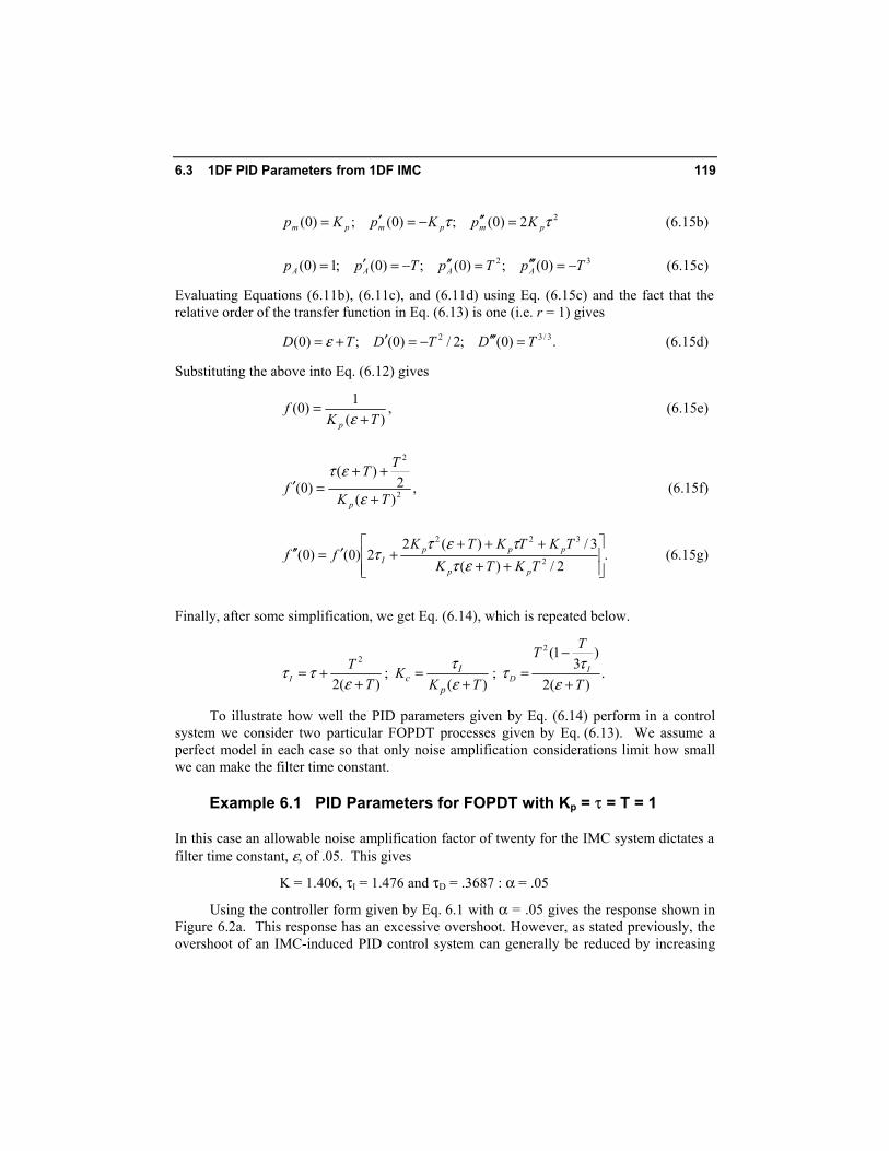
Using the controller form given by Eq. 6.1 with α = .05 gives the response shown in Figure 6.2a. This response has an excessive overshoot. However, as stated previously, the overshoot of an IMC-induced PID control system can generally be reduced by increasing


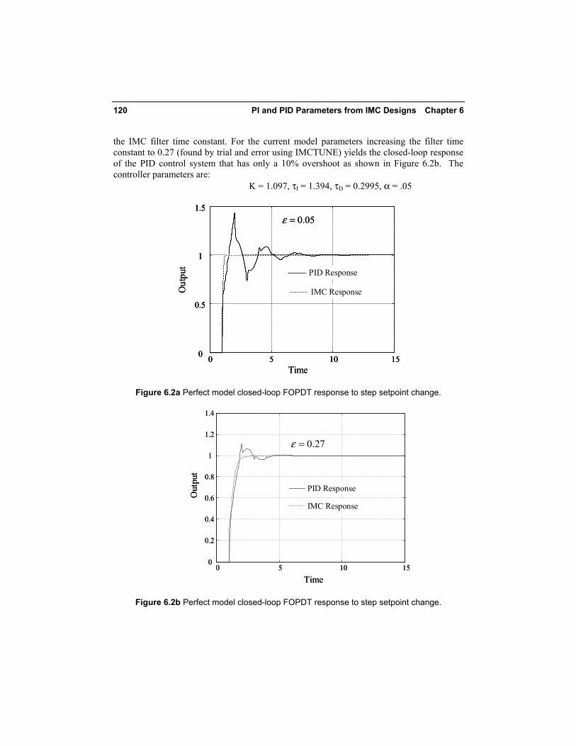
the IMC filter time constant. For the current model parameters increasing the filter time constant to 0.27 (found by trial and error using IMCTUNE) yields the closed-loop response of the PID control system that has only a 10% overshoot as shown in Figure 6.2b. The controller parameters are:

K = 1.097, τI = 1.394, τD = 0.2995, α = .05

0 5 10 150

0.5

1

1.5

Time

Out

put

IMC Response

PID Response

05.0=ε

0 5 10 150 5 10 150

0.5

1

1.5

0

0.5

1

1.5

Time

Out

put

IMC Response

PID Response

05.0=ε

Figure 6.2a Perfect model closed-loop FOPDT response to step setpoint change.

0 5 10 150

0.2

0.4

0.6

0.8

1

1.2

1.4

Time

Out

put

IMC Response

PID Response

27.0=ε

0 5 10 150

0.2

0.4

0.6

0.8

1

1.2

1.4

Time

Out

put

IMC Response

PID Response

27.0=ε

Figure 6.2b Perfect model closed-loop FOPDT response to step setpoint change.


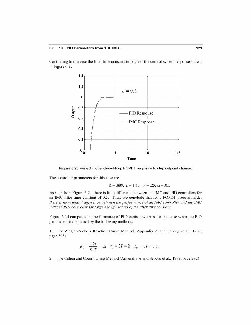
Continuing to increase the filter time constant to .5 gives the control system response shown in Figure 6.2c.

0

0.2

0.4

0.6

0.8

1

1.2

1.4O

utpu

t

0 5 10 15Time

IMC Response

PID Response

5.0=ε

0

0.2

0.4

0.6

0.8

1

1.2

1.4

0

0.2

0.4

0.6

0.8

1

1.2

1.4O

utpu

t

0 5 10 150 5 10 15Time

IMC Response

PID Response

5.0=ε

Figure 6.2c Perfect model closed-loop FOPDT response to step setpoint change.

The controller parameters for this case are

K = .889; τI = 1.33; τD = .25, α = .05.

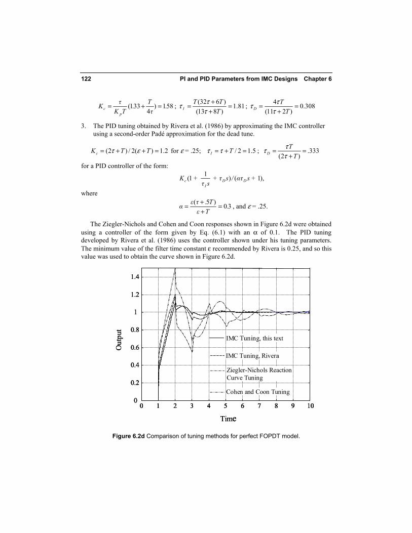
As seen from Figure 6.2c, there is little difference between the IMC and PID controllers for an IMC filter time constant of 0.5. Thus, we conclude that for a FOPDT process model there is no essential difference between the performance of an IMC controller and the IMC induced PID controller for large enough values of the filter time constant,. Figure 6.2d compares the performance of PID control systems for this case when the PID parameters are obtained by the following methods: 1. The Ziegler-Nichols Reaction Curve Method (Appendix A and Seborg et al., 1989, page 303)

2.12.1 ==TK

Kp

cτ 22 == TIτ .5.05. == TDτ

2. The Cohen and Coon Tuning Method (Appendix A and Seborg et al., 1989, page 282)


581)4

331( .τ

T.TKτKp

c =+= ; 81.1)813()632(

=++

=TTT

I τττ ; 308.0

)211(4 =

+=

TT

D τττ

3. The PID tuning obtained by Rivera et al. (1986) by approximating the IMC controller using a second-order Padé approximation for the dead tune.

2.1)(2/)2( =++= TTKc ετ for ε = .25; 5.12/ =+= TI ττ ; 333.)2(

=+

=T

TD τ

ττ

for a PID controller of the form:

),1()11( s + τα/s + τsτ

+ K DDI

c

where

30)5( .Tε

T.τεα =++= , and ε = .25.

The Ziegler-Nichols and Cohen and Coon responses shown in Figure 6.2d were obtained using a controller of the form given by Eq. (6.1) with an α of 0.1. The PID tuning developed by Rivera et al. (1986) uses the controller shown under his tuning parameters. The minimum value of the filter time constant ε recommended by Rivera is 0.25, and so this value was used to obtain the curve shown in Figure 6.2d.

0 1 2 3 4 5 6 7 8 9 100

0.2

0.4

0.6

0.8

1

1.2

1.4

IMC Tuning, this text

Ziegler-Nichols ReactionCurve Tuning

Cohen and Coon Tuning

IMC Tuning, Rivera

Out

put

Time0 1 2 3 4 5 6 7 8 9 100 1 2 3 4 5 6 7 8 9 10

0

0.2

0.4

0.6

0.8

1

1.2

1.4

0

0.2

0.4

0.6

0.8

1

1.2

1.4

IMC Tuning, this textIMC Tuning, this text

Ziegler-Nichols ReactionCurve Tuning

Cohen and Coon Tuning

IMC Tuning, RiveraIMC Tuning, Rivera

Out

put

Time

Figure 6.2d Comparison of tuning methods for perfect FOPDT model.


The response of a control system tuned by the Zeigler-Nichols continuous cycling method (Seborg et al., 1989) lies roughly between the responses of the Zeigler-Nichols reaction curve method and the Cohen and Coon method. It is evident from Figure 6.2d that the IMC tuning methods provide better closed-loop behavior than the traditional tuning methods for the example process. ♦

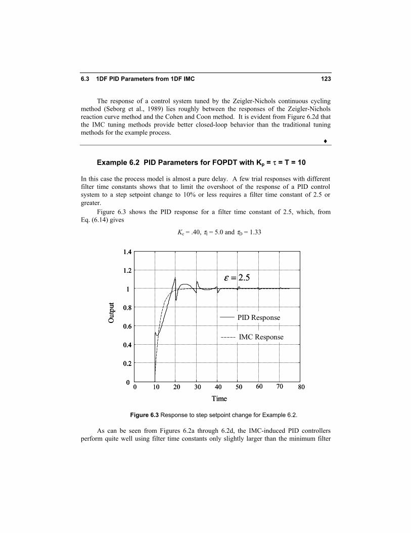
Example 6.2 PID Parameters for FOPDT with Kp = τ = T = 10

In this case the process model is almost a pure delay. A few trial responses with different filter time constants shows that to limit the overshoot of the response of a PID control system to a step setpoint change to 10% or less requires a filter time constant of 2.5 or greater.

Figure 6.3 shows the PID response for a filter time constant of 2.5, which, from Eq. (6.14) gives

Kc = .40, τI = 5.0 and τD = 1.33

0 10 20 30 40 50 800

0.2

0.4

0.6

0.8

1

1.2

1.4

Time

Out

put

60 70

IMC Response

PID Response

5.2=ε

0 10 20 30 40 50 800

0.2

0.4

0.6

0.8

1

1.2

1.4

0

0.2

0.4

0.6

0.8

1

1.2

1.4

Time

Out

put

60 70

IMC Response

PID Response

5.2=ε

Figure 6.3 Response to step setpoint change for Example 6.2.

As can be seen from Figures 6.2a through 6.2d, the IMC-induced PID controllers perform quite well using filter time constants only slightly larger than the minimum filter


time constants required to limit noise amplification to a factor of 20. Thus, for these examples and indeed for most single input, single output systems, there is little or no advantage in dynamic response in implementing an IMC system rather than an IMC-induced PID control system. However, when the dead time is very large relative to the sum of the process time constants, as in Example 6.2, then there is a significant advantage to applying an IMC system. Figure 6.3 shows that the response time of even a well tuned PID control system is at best twice that of an IMC system which uses the minimum filter time constant for the allowable noise amplification (i.e., 0.05 for Example 6.2). ♦

6.4 ALGORITHMS AND SOFTWARE FOR COMPUTING PID PARAMETERS

The analytical expressions for the PID parameters derived in Section 6.3.3 require evaluating several derivatives related to the process model and the feedback form of the IMC controller. Any software package that is capable of evaluating derivatives analytically, such as Mathematica or Maple, can be used to automate this procedure for general models. However, analytical expressions for the PID parameters in terms of the model parameters for general models and controllers are of limited usefulness, and one is usually quite satisfied with numerical values for the PID parameters for a specific model, IMC controller, and filter time constant. In this case there is no need to carry out analytical differentiations, and there are many software tools that can be used to get the desired PID parameters. Recall that the feedback form of the IMC controller, c(s), is given by Eq. (6.5) and is

)()1(

)()(

1

spssp

scA

rm

−+=

−

ε

Substituting Padé approximations for the exponential terms in pm(s) and pA(s) allows us to express these terms as

)(

)()(

*

sDsNK

spm

mpm = ; ,

)()()( *

*

sDsNsp

A

AA = (6.16)

where

.1)0()0()0()0(),0( *** ====≡ AmAmp DDNNpK

Substituting Eq. (6.16) into Eq. (6.5) and clearing fractions gives

.)()1)(()(

)()()( ***

*

sNssDsNKsDsD

scA

rAmp

mA

−+=

ε (6.17a)

6.4 Algorithms and Software for Computing PID Parameters 125

Since the process model )(~ sp is assumed stable, the use of stable Padé approximates

for e-Ts assures that the numerator terms in Eq. (6.17a) (i.e., )(* sDA and )(sDm ) are polynomials with roots in the left half of the s-plane.

The denominator term in Eq. (6.17a) is a polynomial with a zero at the origin, whose coefficients all depend on the filter time constant ε. This polynomial has only stable (i.e., left half plane) zeros once the zero at the origin is factored out, provided that pA(s) is selected so that the magnitude of its frequency response is non-increasing. In this case application of the Nyquist criterion shows that the denominators of Equations (6.5) and (6.17a) have no right half plane zeros. This will always be the case using the design methods suggested in Chapter 3. Therefore, the controller c(s) given by Eq. (6.17a) can be rewritten as

1,)(

)()( 001

0

0 ===

∑

∑−

=

= βαεβ

αε

n

i

ii

n

i

ii

ss

sksc (6.17b)

where

αi, βi ≥ 0 and βi (ε), k(ε) are functions of ε.

Dropping terms higher than second-order in the numerator and higher than third-order in the denominator gives

.)1(

)1)(()(1

22

12

2

++++≅

sssssksc

ββααε (6.18a)

The controller given by Eq. (6.18a) can be viewed as an ideal PID controller cascaded with a second-order lag. The ideal PID controller parameters are

./;)(; 121 ααττεατ === Dici kK (6.18b)

The second-order lag is given by:

1/(β2s2 + β1s +1). (6.18c)

Expanding (6.18a) in a Maclaurin series, as was done in Section 6.3.1, gives

[ ].1)()()( 112

1122

12

sssksc +−+−−+≅ βαβαββα (6.19)

From Eq. (6.19), the parameters of an ideal PID controller are

./)(;; 1122

1211 iDici kK τβαββαττβατ −−+==−= (6.20)

If a sufficiently high-order Padé approximation (a five over five Padé approximation is more than adequate) is used in obtaining Eq. (6.19), then the PID parameters given by


Eq. (6.20) are the same as those given by the combination of Eq. (6.10) as evaluated from Eq. (6.12).

IMCTUNE carries out the manipulations necessary to obtain Eq. (6.17b) from Eq. (6.5) and from there gets the PID parameters given by Eq. (6.20). The input required by IMCTUNE is the process model )(~ sp , the portion of the model to be inverted by the controller pm(s), and the IMC controller filter time constant ε.

6.5 ACCOMMODATING NEGATIVE INTEGRAL AND DERIVATIVE TIME CONSTANTS

The derivative and/or integral time constants computed from Eq. (6.10) or from Eq. (6.20) can be negative for some process models, independent of the choice of filter time constant. This often occurs when the process model has one or more dominant lead time constants, as in Example 6.3.

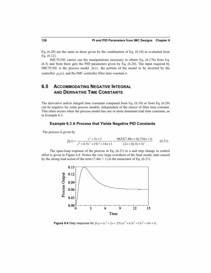
Example 6.3 A Process that Yields Negative PID Constants

The process is given by

3234

2

)15)(.12()1536)(.146.7(0625.

114155.612)(~

++++=

++++++=

ssss

sssssssp (6.21)

The open-loop response of the process in Eq. (6.21) to a unit step change in control effort is given in Figure 6.4. Notice the very large overshoot of the final steady state caused by the strong lead action of the term (7.46s + 1) in the numerator of Eq. (6.21).

0 3 6 9 12 15Time

0.00

0.03

0.06

0.09

0.12

0.15

Proc

ess O

utpu

t

0 3 6 9 12 150 3 6 9 12 15Time

0.00

0.03

0.06

0.09

0.12

0.15

0.00

0.03

0.06

0.09

0.12

0.15

Proc

ess O

utpu

t

Figure 6.4 Step response for )114155.6/()25.2()(~ 2342 ++++++= sssssssp .

6.5 Accommodating Negative Integral and Derivative Time Constants 127

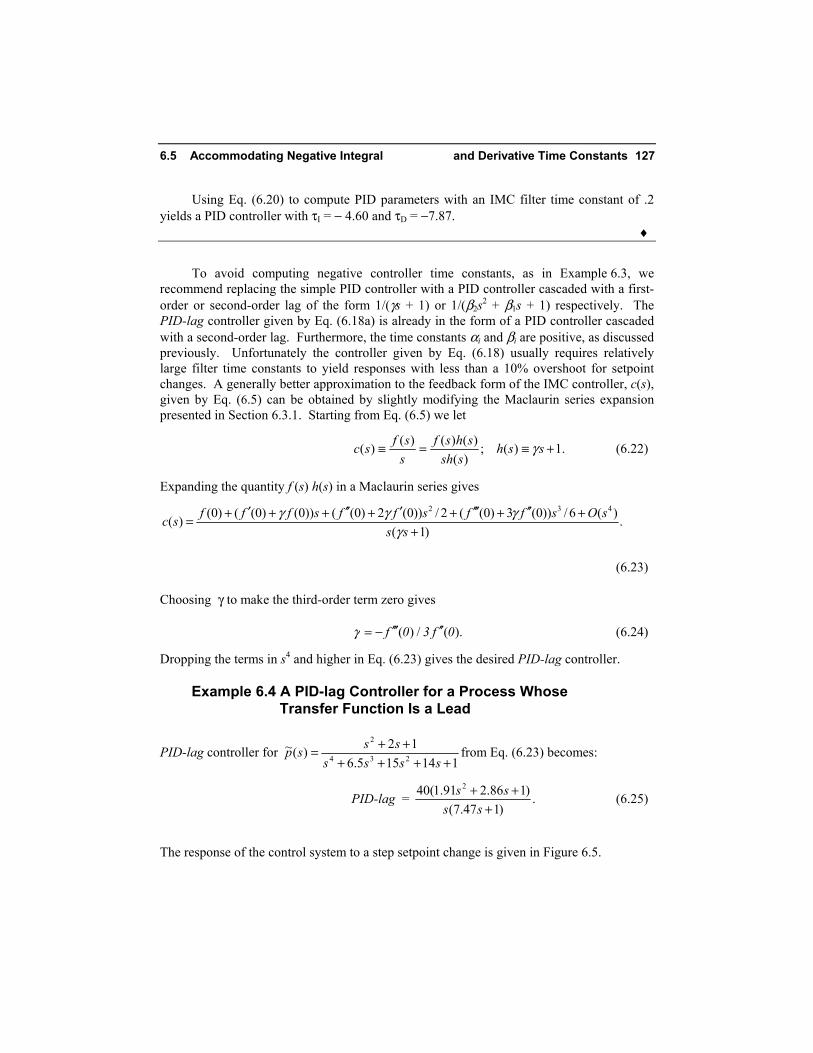
Using Eq. (6.20) to compute PID parameters with an IMC filter time constant of .2 yields a PID controller with τI = − 4.60 and τD = −7.87. ♦

To avoid computing negative controller time constants, as in Example 6.3, we

recommend replacing the simple PID controller with a PID controller cascaded with a first-order or second-order lag of the form 1/(γs + 1) or 1/(β2s2 + β1s + 1) respectively. The PID-lag controller given by Eq. (6.18a) is already in the form of a PID controller cascaded with a second-order lag. Furthermore, the time constants αi and βi are positive, as discussed previously. Unfortunately the controller given by Eq. (6.18) usually requires relatively large filter time constants to yield responses with less than a 10% overshoot for setpoint changes. A generally better approximation to the feedback form of the IMC controller, c(s), given by Eq. (6.5) can be obtained by slightly modifying the Maclaurin series expansion presented in Section 6.3.1. Starting from Eq. (6.5) we let

.1)(;)(

)()()()( +≡=≡ sshssh

shsfssfsc γ (6.22)

Expanding the quantity f (s) h(s) in a Maclaurin series gives

.)1(

)(6/))0(3)0((2/))0(2)0(())0()0(()0()(432

++′′+′′′+′+′′++′+=

sssOsffsffsfffsc

γγγγ

(6.23)

Choosing γ to make the third-order term zero gives

).(/)( 0f30f ′′′′′−=γ (6.24)

Dropping the terms in s4 and higher in Eq. (6.23) gives the desired PID-lag controller.

Example 6.4 A PID-lag Controller for a Process Whose Transfer Function Is a Lead

PID-lag controller for 114155.6

12)(~234

2

++++++=

sssssssp from Eq. (6.23) becomes:

PID-lag = .)147.7(

)186.291.1(40 2

+++

ssss (6.25)

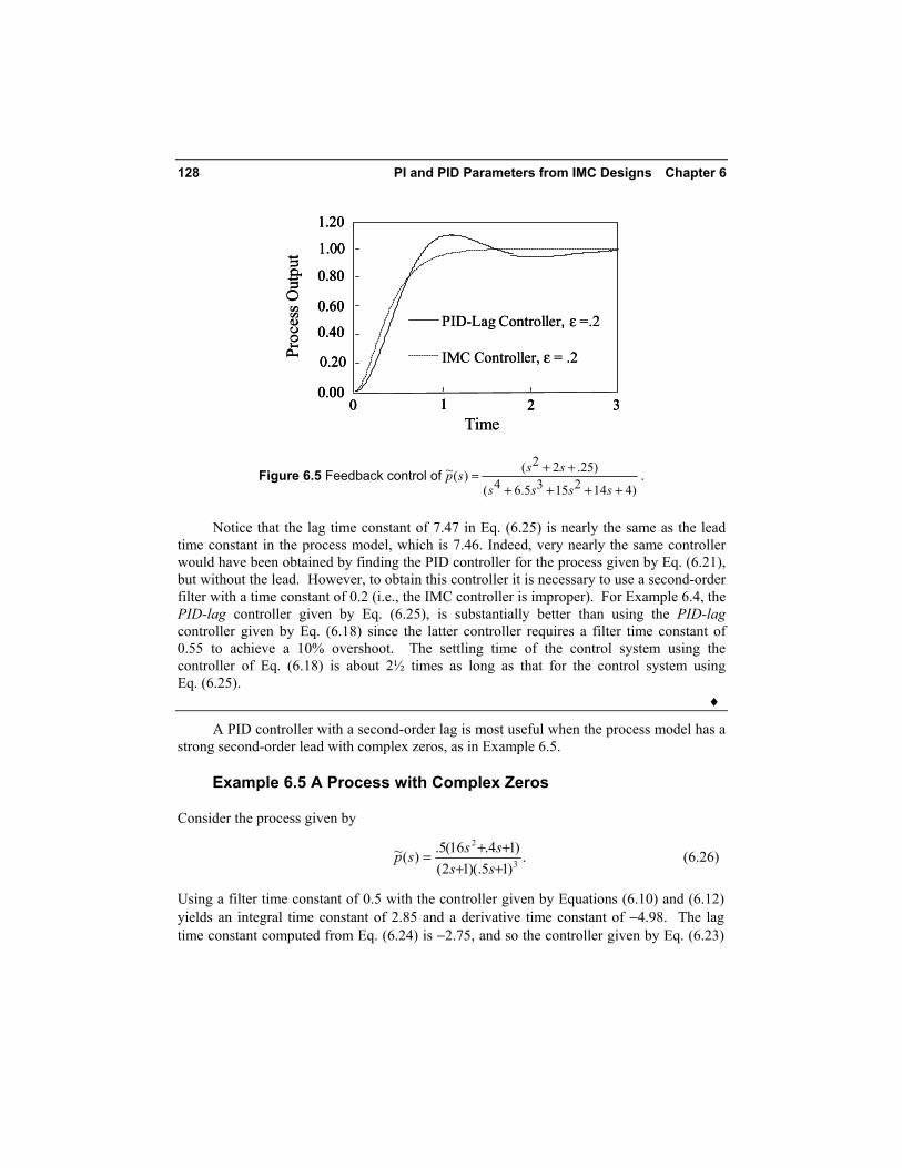
The response of the control system to a step setpoint change is given in Figure 6.5.


0 1 2 3Time

0.00

0.20

0.40

0.60

0.80

1.00

1.20

Proc

ess O

utpu

t

PID-Lag Controller, ε =.2

IMC Controller, ε = .2

0 1 2 30 1 2 3Time

0.00

0.20

0.40

0.60

0.80

1.00

1.20

0.00

0.20

0.40

0.60

0.80

1.00

1.20

Proc

ess O

utpu

t

PID-Lag Controller, ε =.2

IMC Controller, ε = .2

Figure 6.5 Feedback control of)41421535.64(

)25.22()(~++++

++=ssss

sssp .

Notice that the lag time constant of 7.47 in Eq. (6.25) is nearly the same as the lead time constant in the process model, which is 7.46. Indeed, very nearly the same controller would have been obtained by finding the PID controller for the process given by Eq. (6.21), but without the lead. However, to obtain this controller it is necessary to use a second-order filter with a time constant of 0.2 (i.e., the IMC controller is improper). For Example 6.4, the PID-lag controller given by Eq. (6.25), is substantially better than using the PID-lag controller given by Eq. (6.18) since the latter controller requires a filter time constant of 0.55 to achieve a 10% overshoot. The settling time of the control system using the controller of Eq. (6.18) is about 2½ times as long as that for the control system using Eq. (6.25). ♦

A PID controller with a second-order lag is most useful when the process model has a strong second-order lead with complex zeros, as in Example 6.5.

Example 6.5 A Process with Complex Zeros

Consider the process given by

.)15(.)12()14.16(5.)(~3

2

++++=

sssssp (6.26)

Using a filter time constant of 0.5 with the controller given by Equations (6.10) and (6.12) yields an integral time constant of 2.85 and a derivative time constant of −4.98. The lag time constant computed from Eq. (6.24) is −2.75, and so the controller given by Eq. (6.23)


also cannot be used. Finally, the controller given by Eq. (6.18) (for a filter time constant of 0.5) is

PID-lag = .)165.1.16()15.375.3(2

2

2

++++

sssss (6.27)

Notice that the denominator lag of Eq. (6.27) is very close to the numerator lead in the process model given by Eq. (6.26). Here again, if one eliminates the numerator term (16s2 + 4s + 1), the result is

PID-lag = .)1416(

)125.394.2(22

2

++++

sssss (6.28)

The control system response using Eq. (6.28) is very similar to that using Eq. (6.27). ♦

6.6 2DF PID PARAMETERS FROM 2DF IMC

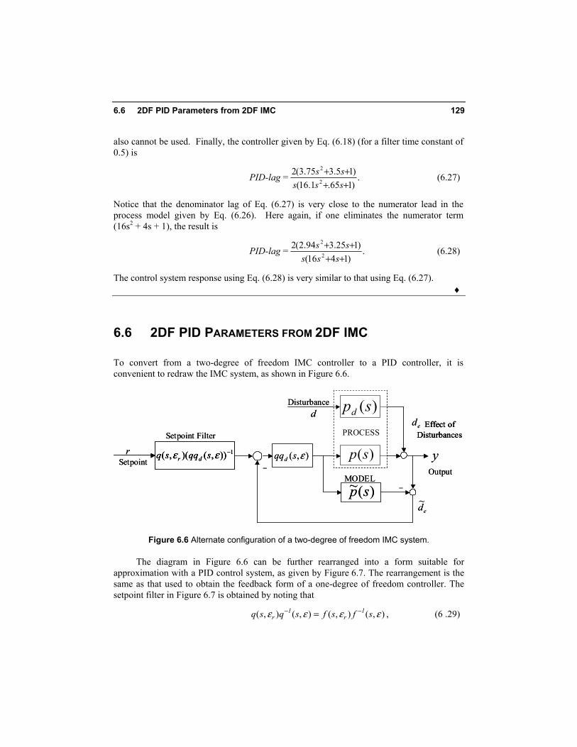
To convert from a two-degree of freedom IMC controller to a PID controller, it is convenient to redraw the IMC system, as shown in Figure 6.6.

Setpoint Filter PROCESS

MODEL

Disturbance

r

Effect ofDisturbances

Output

y

_

),( εsqqd

)(~ sp

)(sp

)(spd

Setpoint1)),()(,( −εε sqqsq dr

_

ded

ed~


MODEL

Disturbance

r



Output

y

_

),( εsqqd

)(~ sp

)(sp

)(spd

Setpoint1)),()(,( −εε sqqsq dr1)),()(,( −εε sqqsq dr

_

ded

ed~

Figure 6.6 Alternate configuration of a two-degree of freedom IMC system.

The diagram in Figure 6.6 can be further rearranged into a form suitable for approximation with a PID control system, as given by Figure 6.7. The rearrangement is the same as that used to obtain the feedback form of a one-degree of freedom controller. The setpoint filter in Figure 6.7 is obtained by noting that

),(),(),(),( εεεε sfsfsqsq 1r

1r

−− = , (6 .29)


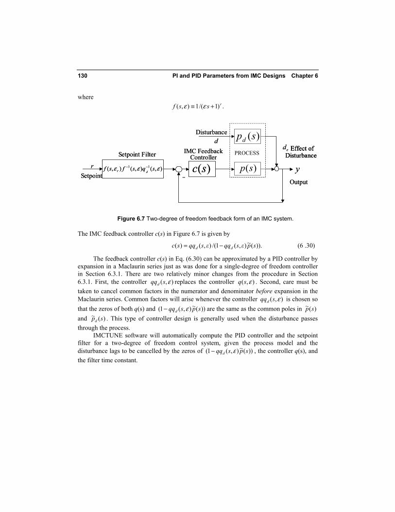
where .)1/(1),( rssf +≡ εε

Setpoint


Disturbance

r


Output

y)(sp

)(spd

),(),(),( 11 εεε sqsfsfdr−−

_)(sc

IMC Feedback Controller

ded

Setpoint


Disturbance

r



Output

y)(sp

)(spd

),(),(),( 11 εεε sqsfsfdr−−

_)(sc

IMC Feedback Controller

ded

Figure 6.7 Two-degree of freedom feedback form of an IMC system.

The IMC feedback controller c(s) in Figure 6.7 is given by

)).(~),(1/(),()( spεsqqεsqqsc dd −= (6 .30)

The feedback controller c(s) in Eq. (6.30) can be approximated by a PID controller by expansion in a Maclaurin series just as was done for a single-degree of freedom controller in Section 6.3.1. There are two relatively minor changes from the procedure in Section 6.3.1. First, the controller ),( εsqqd replaces the controller ),( εsq . Second, care must be taken to cancel common factors in the numerator and denominator before expansion in the Maclaurin series. Common factors will arise whenever the controller ),( εsqqd is chosen so that the zeros of both q(s) and ))(~),(1( spsqqd ε− are the same as the common poles in )(~ sp and )(~ spd . This type of controller design is generally used when the disturbance passes through the process.

IMCTUNE software will automatically compute the PID controller and the setpoint filter for a two-degree of freedom control system, given the process model and the disturbance lags to be cancelled by the zeros of ))(~),(1( spsqqd ε− , the controller q(s), and the filter time constant.

6.7 Saturation Compensation 131

6.7 SATURATION COMPENSATION

No PID controller should be implemented without compensation for the fact that all real control efforts have limits. For example, when a valve opens fully, the flow through the valve usually stops increasing fairly rapidly. When it shuts, the flow through it goes to zero. Most control valves in the U.S. are air operated diaphragm types that operate over an air pressure range of 3 to 15 pounds air pressure (psig) (Smith and Corripio, 1985). The decision whether the valve should be closed (i.e., “air to open”) or open (i.e., “air to close”) at 3 psig is based on maintaining safe operation should air pressure be lost. In any case, the limits of 3 and 15 psig air pressure constitute what are commonly called hard limits, since even if the air pressure can be increased or decreased, the valve ceases to either open or close further. A fully open or closed valve, or indeed any actuator at its limit, is often said to be “saturated.”

Actuator saturation can cause serious problems in the performance of even well-tuned PID control systems that lack special saturation compensation. To illustrate the potential problem, we consider the operation of a PID control system with no saturation compensation. We assume that a disturbance has occurred that cannot be compensated with the available control effort. In this case the error between the setpoint and the measured process variable will be either positive or negative, and the control effort will be at its limit. The uncompensated PID controller will continue to integrate this nonzero error as long as the disturbance persists, and the controller output will continue to grow towards plus or minus infinity. Let us assume that the disturbance decreases to the point where the setpoint can be achieved by the available control effort. Now, however, the controller output signal is substantially above or below the saturation limits of the actuator. Since the disturbance that originally caused actuator saturation is now gone, the error between the setpoint and the process variable has changed sign and the controller has started integrating in the opposite direction. Therefore after some, possibly long, period of time, the controller output will drop below the actuator saturation limit, and the actuator will move away from its limit. The period between the time when the error changed sign and when the actuator moved away from saturation is a controller-induced dead time during which the output was needlessly away from its setpoint. Worse still, if the process variable was sufficiently far from its setpoint during the controller-induced dead time, it is possible that the control effort will saturate at the opposite limit, and the control system will enter a “limit cycle” wherein the control effort cycles continuously between limits. The problem just described is often called reset windup, as the integral action of a PID controller was, and sometimes still is, referred to as reset action.2 A PID controller that has compensation to prevent reset windup is often said to have anti-reset windup compensation.

2 This terminology probably dates back to the earliest proportional-only controllers (gain-only controllers). The operator would adjust (reset) the control effort bias (the value of the controller output when the controller input error is zero) to remove the steady-state error (offset) between the setpoint and process variable. Such offsets are characteristic of proportional-only control systems when there are changes in disturbances or the setpoint.


There are two types of anti-reset windup compensation. The most common type of compensation is a digital implementation of an older analog implementation of the integral action, wherein the integral action is obtained by positive feedback of a first-order lag around a limiter that has a gain of one in its linear region. This type of anti-reset windup compensation will be described in some detail in this section. A less common form of anti-reset windup is one where the integration stops as soon as the controller output saturates. The integration is restarted when either the error between the setpoint and process variable changes sign, or the control effort comes off saturation, possibly due to a change in control effort bias or in some other external signal, such as that from a feedforward controller.

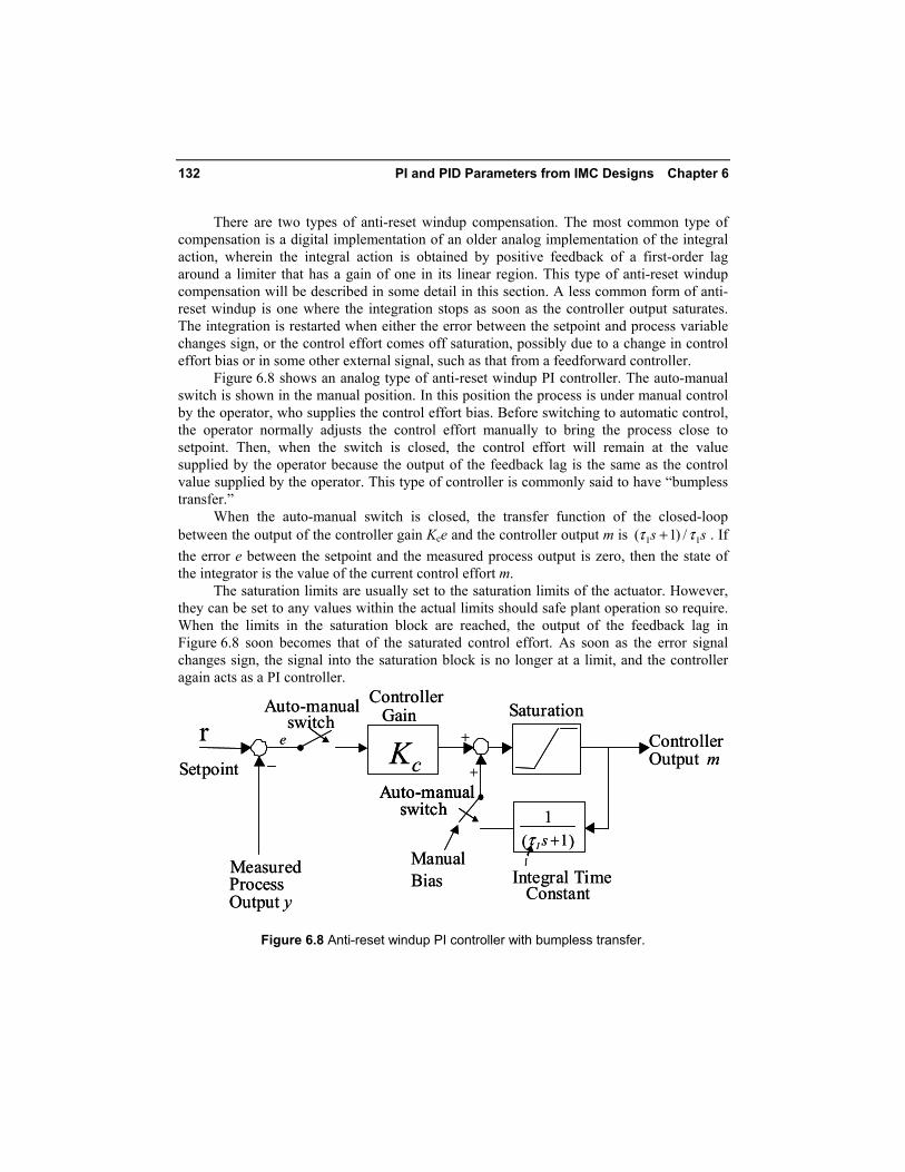
Figure 6.8 shows an analog type of anti-reset windup PI controller. The auto-manual switch is shown in the manual position. In this position the process is under manual control by the operator, who supplies the control effort bias. Before switching to automatic control, the operator normally adjusts the control effort manually to bring the process close to setpoint. Then, when the switch is closed, the control effort will remain at the value supplied by the operator because the output of the feedback lag is the same as the control value supplied by the operator. This type of controller is commonly said to have “bumpless transfer.”

When the auto-manual switch is closed, the transfer function of the closed-loop between the output of the controller gain Kce and the controller output m is ss II /)1( ττ + . If the error e between the setpoint and the measured process output is zero, then the state of the integrator is the value of the current control effort m.

The saturation limits are usually set to the saturation limits of the actuator. However, they can be set to any values within the actual limits should safe plant operation so require. When the limits in the saturation block are reached, the output of the feedback lag in Figure 6.8 soon becomes that of the saturated control effort. As soon as the error signal changes sign, the signal into the saturation block is no longer at a limit, and the controller again acts as a PI controller.

rController

Gain

Kc

Saturation

)(1

+

+Auto-manual

switch

ControllerOutput m

Integral TimeConstant

Setpoint

MeasuredProcess Output y

e

Auto-manualswitch

Manual Bias

1+sIτ

rController

Gain

Kc

Saturation

)(1

+

+Auto-manual

switchAuto-manual

switch

ControllerOutput m


Setpoint

MeasuredProcess Output y

e

Auto-manualswitch

Manual Bias

1+sIτ

Figure 6.8 Anti-reset windup PI controller with bumpless transfer.

6.8 Summary 133

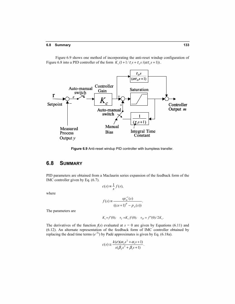
Figure 6.9 shows one method of incorporating the anti-reset windup configuration of Figure 6.8 into a PID controller of the form ))1/(/11( DDI +++ sssKc ατττ .

rController

Gain

Kc

Saturation

)(1

+

+Auto-manual

switch

ControllerOutput m


Setpoint

MeasuredProcess

e

Auto-manualswitch

Manual Bias

1+sIτ

)1( +ss

D

D

αττ

Output y

rController

Gain

Kc

Saturation

)(1

+

+Auto-manual

switchAuto-manual

switch

ControllerOutput mControllerOutput m


Setpoint

MeasuredProcess

e

Auto-manualswitch

Manual Bias

1+sIτ

)1( +ss

D

D

αττ

Output y

Figure 6.9 Anti-reset windup PID controller with bumpless transfer.

6.8 SUMMARY

PID parameters are obtained from a Maclaurin series expansion of the feedback form of the IMC controller given by Eq. (6.7). ),(1)( sf

ssc ≡

where

.))()1((

)()(

1

sprεs

sspsf

A

m

−+≡

−

The parameters are

.2)0()0()0( cDcIc K/''fτ;/fKτ;'fK ===

The derivatives of the function f(s) evaluated at s = 0 are given by Equations (6.11) and (6.12). An alternate representation of the feedback form of IMC controller obtained by replacing the dead time terms (e-Ts) by Padé approximates is given by Eq. (6.18a).

.)1(

)1)(()(1

22

12

2

++++≅

sssssksc

ββααε


In terms of Eq. (6.18a), the PID parameters are given by Eq. (6.20).

./)(;; 1122

1211 iDici kK τβαββαττβατ −−+==−=

If either, or both, τI or τD are negative, then a PID-lag controller should be used. The controllers, in order of preference, are given by Equations (6.23) and (6.18a). If any of the time constants in Eq. (6.23) are negative, then use the controller given by Eq. (6.18a).

Problems 6.1 Show that the combination of Equations (6.2) and (6.3) yields Eq. (6.1).

6.2 Derive an analytical expression for the PID parameters in terms of the process parameters for

( ).12)( 22 +τζ+τ

=−

sseKsp

TS

6.3 Derive the PI parameters for

a) a pure time delay process

b) the process given in Problem 6.2.

6.4 Select PID or PID-lag controllers for each of the problems in Chapter 3. Use the smallest filter time constant that limits the closed-loop overshoot to 10% for a step setpoint change. Note that such a filter time constant can actually be smaller than the IMC filter time constant required by the IMC controller, since a PID controller never amplifies high frequency noise by more than 20 by the manner in which the derivative action is implemented.

6.5 Select two-degree of freedom PID controllers where appropriate for each of the problems in Chapter 3, assuming that the disturbance enters through the process. If a two-degree of freedom PID controller is not appropriate, explain why.

6.6 Derive the closed-loop transfer function for Figure 6.9.

References

Morari, M., and F. Zafiriou. 1989. Robust Process Control. Chapter, Prentice-Hall, NJ

Rivera, D. E., S. Skogestad, and M. Morari. 1986. “Internal Model Control 4. PID Controller Design,” I&EC Chem. Proc. Des. & Dev. 25, 252–265.

Seborg, D. E., T. F. Edgar, and D. A. Mellichamp. 1989. Process Dynamics and Control, John Wiley & Sons, NY.

Smith, C. A., and A. B. Corripio. 1985. Principles and Practice of Automatic Process Control. John Wiley & Sons, NY.

PI and PID Parameters from IMC Designs - BGU courses/Chapter 6... · PI and PID Parameters from IMC...

Documents

Transcript of PI and PID Parameters from IMC Designs - BGU courses/Chapter 6... · PI and PID Parameters from IMC...