Physics of gamma-ray loud AGN jets through high cadence, multi-frequency polarization monitoring

Ioannis Myserlis

E. Angelakis, L. Fuhrmann, A. Kraus, V. Pavlidou, D. Blinov, V. Karamanavis, J. A. Zensus

s+ 1

s+ 73

3

6s+ 13

↵ = �s� 1

2

||

⏊

↵ = +2.5

based on Pacholczyk (1977)

χ perpendicular to projected B-field

χ parallel to projected B-field

N(E)dE = E�sdE

S⌫ / ⌫�s�12 = ⌫�a

Energy distribution

S(⌫) / ⌫↵

2

Synchrotron polarization

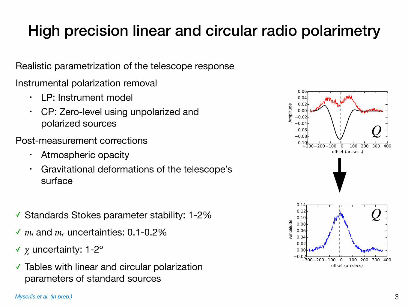
High precision linear and circular radio polarimetry

Realistic parametrization of the telescope responseInstrumental polarization removal

• LP: Instrument model• CP: Zero-level using unpolarized and

polarized sourcesPost-measurement corrections

• Atmospheric opacity• Gravitational deformations of the telescope’s

surface

✓ Standards Stokes parameter stability: 1-2%✓ ml and mc uncertainties: 0.1-0.2%✓ χ uncertainty: 1-2º✓ Tables with linear and circular polarization

parameters of standard sourcesAm

plitu

de

Q

Ampl

itude

Q

3Myserlis et al. (in prep.)

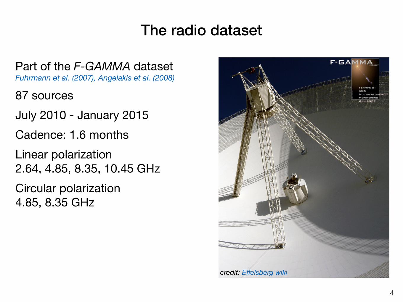
Part of the F-GAMMA datasetFuhrmann et al. (2007), Angelakis et al. (2008)87 sourcesJuly 2010 - January 2015Cadence: 1.6 monthsLinear polarization2.64, 4.85, 8.35, 10.45 GHzCircular polarization4.85, 8.35 GHz

The radio dataset

4

credit: Effelsberg wiki

4.3. DERIVATIVE QUANTITIES 83

Figure 4.8: Histograms of the magnetic field strength for sources with at least one |mc| datapoint of high significance (signal-to-noise ratio ≥ 3). The plots have been truncated to 60 mGto ease reading. There is one data point outside the given ranges for the 4.85 GHz data.

various VLBI components position angles, given in [Lister et al., 2013], for all the availablesources.

As a cross-check we compared our median RM values with the ones given in[Taylor et al., 2009] which were computed from the NVSS data. The comparison plot is shownin Fig. 4.9. The RM differences between the two projects have a median value of 19.7 rad m−2.A Spearman ρ test reveals a very significant correlation (p = 2 · 10−5) of ρ = 0.63, suggestinga good agreement between the two projects.

The physical interpretation of the RM

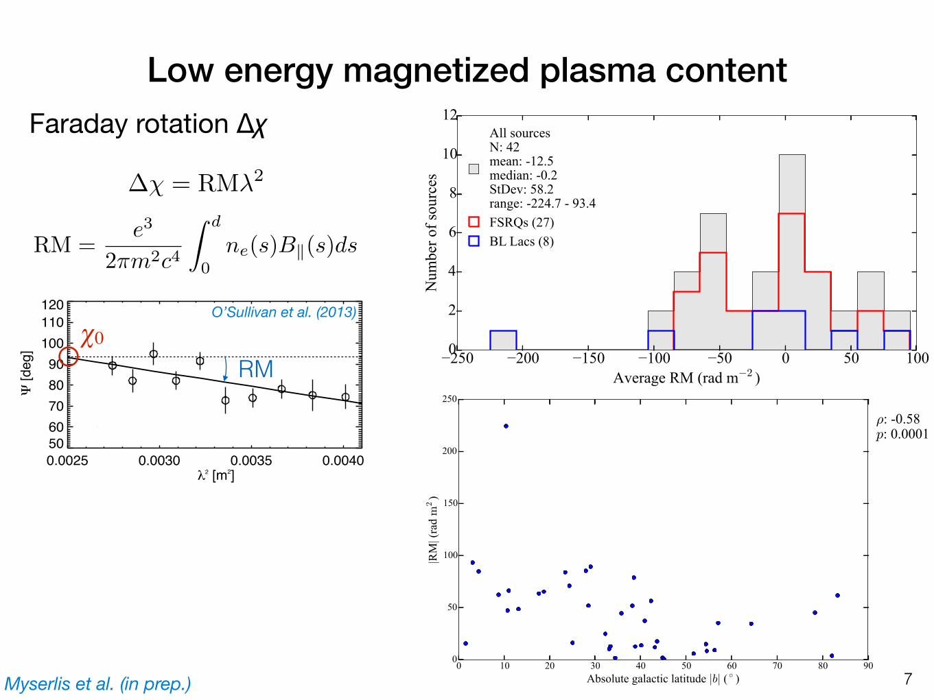
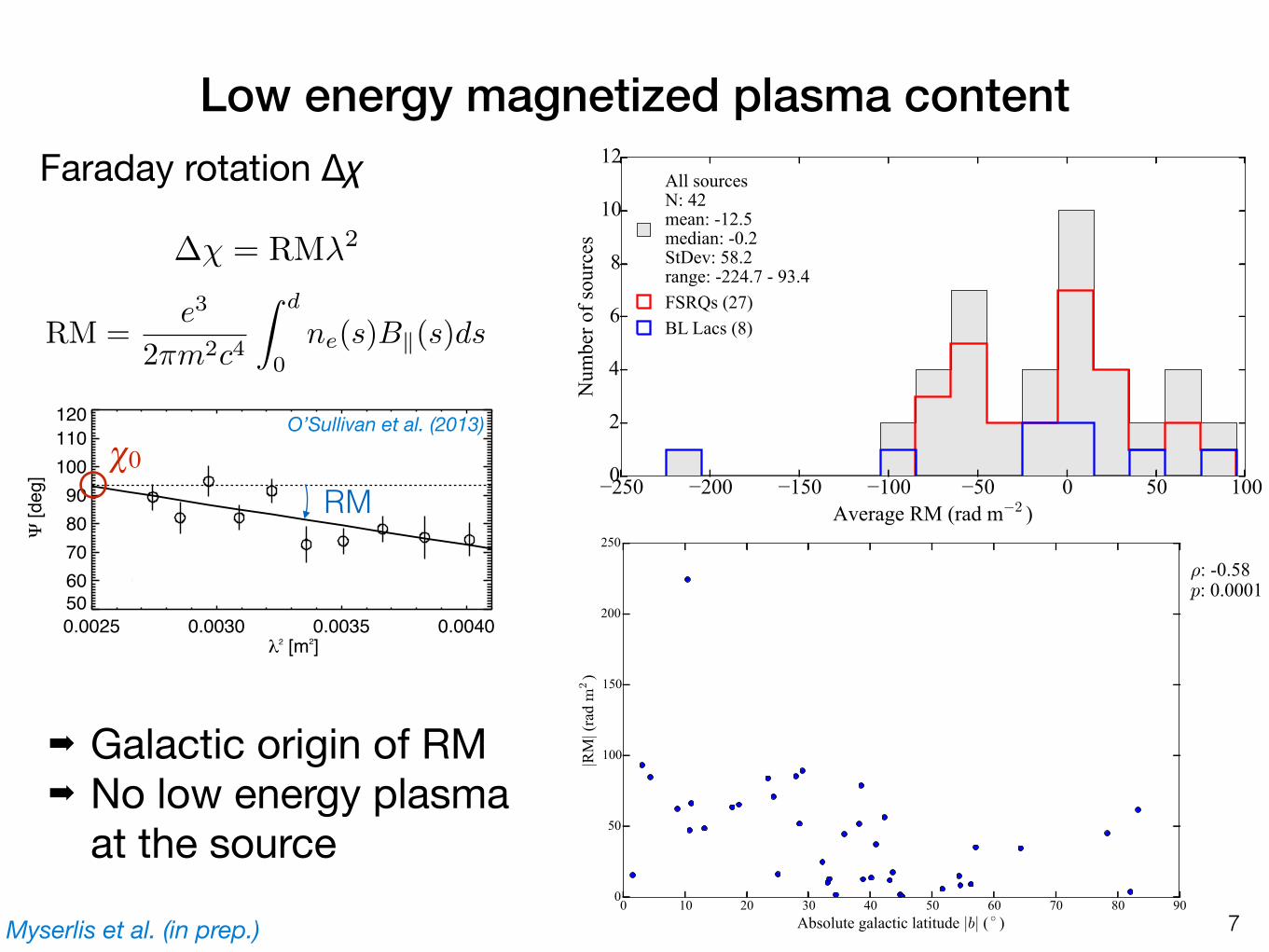
A histogram of the RM values we estimated for all sources is given in Fig. 4.10. The ma-jority of the estimated RM values lie in the range between ± 100 rad m−2. Those levels areconsistent with the interpretation that the Faraday effect mainly takes place in the magnetizedplasma of our Galaxy, since the observed rotation measures are similar to the galactic levels[Taylor et al., 2009]. In Fig. 4.11, we give a celestial map for the sources we estimated therotation measure in galactic coordinates and in Fig. 4.12 we plot the absolute rotation measureas a function of the absolute galactic latitude, |b| for each source. We performed a Spearmanρ test for the latter datasets which showed a very significant correlation of ρ = −0.58 with a99.99 % confidence level. This is in accordance with the assumption for the galactic origin ofthe rotation measure.

Assumptions• Synchrotron circular

polarization• One particle population,

e.g. e- or e+

• Uniform magnetic field

4.3. DERIVATIVE QUANTITIES 83

Figure 4.8: Histograms of the magnetic field strength for sources with at least one |mc| datapoint of high significance (signal-to-noise ratio ≥ 3). The plots have been truncated to 60 mGto ease reading. There is one data point outside the given ranges for the 4.85 GHz data.

various VLBI components position angles, given in [Lister et al., 2013], for all the availablesources.

As a cross-check we compared our median RM values with the ones given in[Taylor et al., 2009] which were computed from the NVSS data. The comparison plot is shownin Fig. 4.9. The RM differences between the two projects have a median value of 19.7 rad m−2.A Spearman ρ test reveals a very significant correlation (p = 2 · 10−5) of ρ = 0.63, suggestinga good agreement between the two projects.

The physical interpretation of the RM

A histogram of the RM values we estimated for all sources is given in Fig. 4.10. The ma-jority of the estimated RM values lie in the range between ± 100 rad m−2. Those levels areconsistent with the interpretation that the Faraday effect mainly takes place in the magnetizedplasma of our Galaxy, since the observed rotation measures are similar to the galactic levels[Taylor et al., 2009]. In Fig. 4.11, we give a celestial map for the sources we estimated therotation measure in galactic coordinates and in Fig. 4.12 we plot the absolute rotation measureas a function of the absolute galactic latitude, |b| for each source. We performed a Spearmanρ test for the latter datasets which showed a very significant correlation of ρ = −0.58 with a99.99 % confidence level. This is in accordance with the assumption for the galactic origin ofthe rotation measure.

5

Homan et al. (2009)

Myserlis et al. (in prep.)

B ⇠ m2

c⌫obs(1 + z)

2.8D

Magnetic field strength

4.3. DERIVATIVE QUANTITIES 83

Figure 4.8: Histograms of the magnetic field strength for sources with at least one |mc| datapoint of high significance (signal-to-noise ratio ≥ 3). The plots have been truncated to 60 mGto ease reading. There is one data point outside the given ranges for the 4.85 GHz data.

various VLBI components position angles, given in [Lister et al., 2013], for all the availablesources.

As a cross-check we compared our median RM values with the ones given in[Taylor et al., 2009] which were computed from the NVSS data. The comparison plot is shownin Fig. 4.9. The RM differences between the two projects have a median value of 19.7 rad m−2.A Spearman ρ test reveals a very significant correlation (p = 2 · 10−5) of ρ = 0.63, suggestinga good agreement between the two projects.

The physical interpretation of the RM

A histogram of the RM values we estimated for all sources is given in Fig. 4.10. The ma-jority of the estimated RM values lie in the range between ± 100 rad m−2. Those levels areconsistent with the interpretation that the Faraday effect mainly takes place in the magnetizedplasma of our Galaxy, since the observed rotation measures are similar to the galactic levels[Taylor et al., 2009]. In Fig. 4.11, we give a celestial map for the sources we estimated therotation measure in galactic coordinates and in Fig. 4.12 we plot the absolute rotation measureas a function of the absolute galactic latitude, |b| for each source. We performed a Spearmanρ test for the latter datasets which showed a very significant correlation of ρ = −0.58 with a99.99 % confidence level. This is in accordance with the assumption for the galactic origin ofthe rotation measure.

Assumptions• Synchrotron circular

polarization• One particle population,

e.g. e- or e+

• Uniform magnetic field

4.3. DERIVATIVE QUANTITIES 83

Figure 4.8: Histograms of the magnetic field strength for sources with at least one |mc| datapoint of high significance (signal-to-noise ratio ≥ 3). The plots have been truncated to 60 mGto ease reading. There is one data point outside the given ranges for the 4.85 GHz data.

various VLBI components position angles, given in [Lister et al., 2013], for all the availablesources.

As a cross-check we compared our median RM values with the ones given in[Taylor et al., 2009] which were computed from the NVSS data. The comparison plot is shownin Fig. 4.9. The RM differences between the two projects have a median value of 19.7 rad m−2.A Spearman ρ test reveals a very significant correlation (p = 2 · 10−5) of ρ = 0.63, suggestinga good agreement between the two projects.

The physical interpretation of the RM

A histogram of the RM values we estimated for all sources is given in Fig. 4.10. The ma-jority of the estimated RM values lie in the range between ± 100 rad m−2. Those levels areconsistent with the interpretation that the Faraday effect mainly takes place in the magnetizedplasma of our Galaxy, since the observed rotation measures are similar to the galactic levels[Taylor et al., 2009]. In Fig. 4.11, we give a celestial map for the sources we estimated therotation measure in galactic coordinates and in Fig. 4.12 we plot the absolute rotation measureas a function of the absolute galactic latitude, |b| for each source. We performed a Spearmanρ test for the latter datasets which showed a very significant correlation of ρ = −0.58 with a99.99 % confidence level. This is in accordance with the assumption for the galactic origin ofthe rotation measure.

5

Homan et al. (2009)

Myserlis et al. (in prep.)

B ⇠ m2

c⌫obs(1 + z)

2.8D

➡ Median B: 3-6 mG

Magnetic field strength

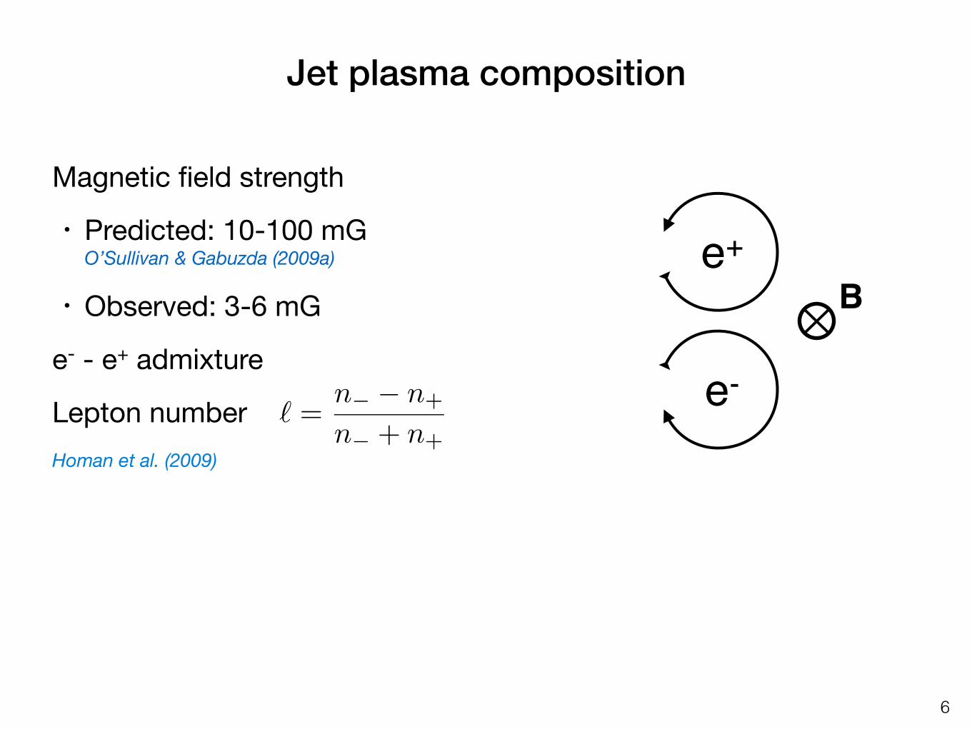
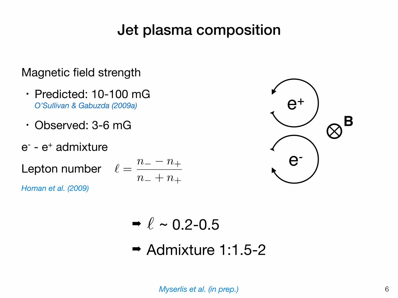
Magnetic field strength• Predicted: 10-100 mG

O’Sullivan & Gabuzda (2009a)• Observed: 3-6 mG

e- - e+ admixtureLepton number

90 CHAPTER 4. RADIO LINEAR AND CIRCULAR POLARIZATION OF AGN JETS

4.4.3 Linear and circular polarization versus RMIn Figures 4.15 and Fig. 4.16, we plot the median ml and the median absolute mc againstthe estimated absolute rotation measure values for our sources. We have considered only thedata points with absolute RM less than 200 rad m−2. Faraday rotation theory predicts an anti-correlation of the observed ml and the RM if the effect is taking place in the source (internalFaraday Rotation) due to differential rotations of the EVPAs for radiation emitted at the samefrequency but different depths. If not, the Faraday rotation effect is taking place mainly exter-nally to the source in a magnetized plasma region along the light path.

For the ml data, we observe a slight anti-correlation with RM only at the the lowest ob-serving frequency with confidence level of 91 %. For the higher frequencies, no correlationis found. This result suggests that at the lowest frequencies we may be affected by internalFaraday rotation in the vicinity of the emitting region, while at the higher ones, the observedRM is caused by external Faraday rotation, possibly due to the low energy magnetized plasmacontent of our Galaxy as found also in subsection 4.3.2. The fact that we may observe internalFaraday rotation at the lowest frequency may be an indication of the presence of low energyplasma at the outer parts of the AGN jets where this emission is mainly coming from.

For the mc data, we don’t get a significant correlation or anti-correlation with RM. Thefact that mc is not correlated with RM, speaks in favor of the observed mc being intrinsicto the synchrotron emission. If it were created by propagation effects it would require lowenergy magnetized plasma which would cause also the observed Faraday rotation. This fact isin accordance with the findings of subsection 4.4.2.

Jet plasma composition

In the light of the previous discussion one can argue that the magnetic field strengths calculatedin subsection 4.3.1 are direct estimates of the magnetic field at the emission region, under theassumption that the emitting plasma is purely consisting of electrons. We can compare thesevalues with the ones predicted by theory under the same assumptions. If the measured mc isless than expected, we can attribute this discrepancy to the presence of positrons in the emittingplasma particles which lower the emitted circular polarization due to their reverse rotation inthe source’s magnetic field.

Finally using the theoretical predictions, we can estimate the ratio of electrons to positronswe need to have in the emitting region to get the observed mc values. This ratio is usuallyexpressed as by the lepton number

ℓ =n− − n+

n− + n+(4.8)

with n− and n+ the electron and positron number density respectively. In this case the observedmc is proportional to ℓ, which makes the magnetic field strength proportional to ℓ2. Sincewe considered only the median of the absolute mc to estimate the magnetic field strength,we cannot discern between electron or positron dominated plasmas but we can estimate theabsolute value of number ℓ. For example, if we assume that theory predicts a magnetic fieldstrength of 10 – 100 mG for an electron plasma [O’Sullivan and Gabuzda, 2009a], and weobserve a median value of ∼ 3 mG at 4.85 GHz (subsection 4.3.1), we calculate that |ℓ| ∼ 0.2– 0.5. This lepton number range shows that for every particle of one population there are 1.5– 2 particles of the other (electrons or positrons). In other words, the admixture of positrons inelectron-dominated jet plasmas or electrons in positron-dominated ones is ∼ 33 – 40%.

4.4.4 Polarization degree versus low and high frequency emission characteristicsThe AGN jet emission is extremely broadband and contains two dominant components. Thelow frequency component is attributed to the incoherent synchrotron emission mechanism

6

Be+

e-

Homan et al. (2009)

Jet plasma composition

Magnetic field strength• Predicted: 10-100 mG

O’Sullivan & Gabuzda (2009a)• Observed: 3-6 mG

e- - e+ admixtureLepton number

90 CHAPTER 4. RADIO LINEAR AND CIRCULAR POLARIZATION OF AGN JETS

4.4.3 Linear and circular polarization versus RMIn Figures 4.15 and Fig. 4.16, we plot the median ml and the median absolute mc againstthe estimated absolute rotation measure values for our sources. We have considered only thedata points with absolute RM less than 200 rad m−2. Faraday rotation theory predicts an anti-correlation of the observed ml and the RM if the effect is taking place in the source (internalFaraday Rotation) due to differential rotations of the EVPAs for radiation emitted at the samefrequency but different depths. If not, the Faraday rotation effect is taking place mainly exter-nally to the source in a magnetized plasma region along the light path.

For the ml data, we observe a slight anti-correlation with RM only at the the lowest ob-serving frequency with confidence level of 91 %. For the higher frequencies, no correlationis found. This result suggests that at the lowest frequencies we may be affected by internalFaraday rotation in the vicinity of the emitting region, while at the higher ones, the observedRM is caused by external Faraday rotation, possibly due to the low energy magnetized plasmacontent of our Galaxy as found also in subsection 4.3.2. The fact that we may observe internalFaraday rotation at the lowest frequency may be an indication of the presence of low energyplasma at the outer parts of the AGN jets where this emission is mainly coming from.

For the mc data, we don’t get a significant correlation or anti-correlation with RM. Thefact that mc is not correlated with RM, speaks in favor of the observed mc being intrinsicto the synchrotron emission. If it were created by propagation effects it would require lowenergy magnetized plasma which would cause also the observed Faraday rotation. This fact isin accordance with the findings of subsection 4.4.2.

Jet plasma composition

In the light of the previous discussion one can argue that the magnetic field strengths calculatedin subsection 4.3.1 are direct estimates of the magnetic field at the emission region, under theassumption that the emitting plasma is purely consisting of electrons. We can compare thesevalues with the ones predicted by theory under the same assumptions. If the measured mc isless than expected, we can attribute this discrepancy to the presence of positrons in the emittingplasma particles which lower the emitted circular polarization due to their reverse rotation inthe source’s magnetic field.

Finally using the theoretical predictions, we can estimate the ratio of electrons to positronswe need to have in the emitting region to get the observed mc values. This ratio is usuallyexpressed as by the lepton number

ℓ =n− − n+

n− + n+(4.8)

with n− and n+ the electron and positron number density respectively. In this case the observedmc is proportional to ℓ, which makes the magnetic field strength proportional to ℓ2. Sincewe considered only the median of the absolute mc to estimate the magnetic field strength,we cannot discern between electron or positron dominated plasmas but we can estimate theabsolute value of number ℓ. For example, if we assume that theory predicts a magnetic fieldstrength of 10 – 100 mG for an electron plasma [O’Sullivan and Gabuzda, 2009a], and weobserve a median value of ∼ 3 mG at 4.85 GHz (subsection 4.3.1), we calculate that |ℓ| ∼ 0.2– 0.5. This lepton number range shows that for every particle of one population there are 1.5– 2 particles of the other (electrons or positrons). In other words, the admixture of positrons inelectron-dominated jet plasmas or electrons in positron-dominated ones is ∼ 33 – 40%.

4.4.4 Polarization degree versus low and high frequency emission characteristicsThe AGN jet emission is extremely broadband and contains two dominant components. Thelow frequency component is attributed to the incoherent synchrotron emission mechanism

6

Be+

e-

Homan et al. (2009)

➡ ~ 0.2-0.5➡ Admixture 1:1.5-2

90 CHAPTER 4. RADIO LINEAR AND CIRCULAR POLARIZATION OF AGN JETS

4.4.3 Linear and circular polarization versus RMIn Figures 4.15 and Fig. 4.16, we plot the median ml and the median absolute mc againstthe estimated absolute rotation measure values for our sources. We have considered only thedata points with absolute RM less than 200 rad m−2. Faraday rotation theory predicts an anti-correlation of the observed ml and the RM if the effect is taking place in the source (internalFaraday Rotation) due to differential rotations of the EVPAs for radiation emitted at the samefrequency but different depths. If not, the Faraday rotation effect is taking place mainly exter-nally to the source in a magnetized plasma region along the light path.

For the ml data, we observe a slight anti-correlation with RM only at the the lowest ob-serving frequency with confidence level of 91 %. For the higher frequencies, no correlationis found. This result suggests that at the lowest frequencies we may be affected by internalFaraday rotation in the vicinity of the emitting region, while at the higher ones, the observedRM is caused by external Faraday rotation, possibly due to the low energy magnetized plasmacontent of our Galaxy as found also in subsection 4.3.2. The fact that we may observe internalFaraday rotation at the lowest frequency may be an indication of the presence of low energyplasma at the outer parts of the AGN jets where this emission is mainly coming from.

For the mc data, we don’t get a significant correlation or anti-correlation with RM. Thefact that mc is not correlated with RM, speaks in favor of the observed mc being intrinsicto the synchrotron emission. If it were created by propagation effects it would require lowenergy magnetized plasma which would cause also the observed Faraday rotation. This fact isin accordance with the findings of subsection 4.4.2.

Jet plasma composition

In the light of the previous discussion one can argue that the magnetic field strengths calculatedin subsection 4.3.1 are direct estimates of the magnetic field at the emission region, under theassumption that the emitting plasma is purely consisting of electrons. We can compare thesevalues with the ones predicted by theory under the same assumptions. If the measured mc isless than expected, we can attribute this discrepancy to the presence of positrons in the emittingplasma particles which lower the emitted circular polarization due to their reverse rotation inthe source’s magnetic field.

Finally using the theoretical predictions, we can estimate the ratio of electrons to positronswe need to have in the emitting region to get the observed mc values. This ratio is usuallyexpressed as by the lepton number

ℓ =n− − n+

n− + n+(4.8)

with n− and n+ the electron and positron number density respectively. In this case the observedmc is proportional to ℓ, which makes the magnetic field strength proportional to ℓ2. Sincewe considered only the median of the absolute mc to estimate the magnetic field strength,we cannot discern between electron or positron dominated plasmas but we can estimate theabsolute value of number ℓ. For example, if we assume that theory predicts a magnetic fieldstrength of 10 – 100 mG for an electron plasma [O’Sullivan and Gabuzda, 2009a], and weobserve a median value of ∼ 3 mG at 4.85 GHz (subsection 4.3.1), we calculate that |ℓ| ∼ 0.2– 0.5. This lepton number range shows that for every particle of one population there are 1.5– 2 particles of the other (electrons or positrons). In other words, the admixture of positrons inelectron-dominated jet plasmas or electrons in positron-dominated ones is ∼ 33 – 40%.

4.4.4 Polarization degree versus low and high frequency emission characteristicsThe AGN jet emission is extremely broadband and contains two dominant components. Thelow frequency component is attributed to the incoherent synchrotron emission mechanism

Myserlis et al. (in prep.)

Jet plasma composition

CP spectrum of PKSB2126–158 5

0.0 0.2 0.4 0.6 0.8 1.0 1.2p [%]

0.4

0.6

0.8

1.0

1.2

mc [

%]

Figure 3. Plot of degree of linear polarization (p) versus thedegree of circular polarization (mc) at each frequency measure-ment. A Spearman rank correlation of −0.8 quantifies the stronganti-correlation between the two variables. The dashed line (red)represents the best-fit power-law with mc ∝ p−0.24±0.03.

is important to note that this source appears to have flaredaround 20091 with its 5 GHz Stokes I flux increasing to itscurrent level of ∼1.7 Jy. However, the amount of Stokes Vappears to have changed very little, since the decrease inmc from ∼1.4% (Rayner 2000) to ∼0.9% at 4.8 GHz can beexplained almost purely by the increase in the Stokes I fluxalone.

3.2 Consideration of the Linearly Polarized

Emission

Figure 1d,e shows the frequency dependence of the linearpolarized emission over the same range as the total inten-sity and circular polarization. We note the low degree oflinear polarization (p ! 0.2%) from 4.5 to 6.5 GHz and thesurprisingly steep rise toward p ∼ 1% at both ends of theband, as well the non-monotonic distribution of linear polar-ization angles (Ψ) with frequency. Assuming that the linearpolarized emission we detect is coming from the same regionof the jet as the CP, then the ratio of mc to p also reachessurprisingly large values, ranging from ∼0.5 to ∼10 acrossour full frequency coverage.

The inverted spectrum of the Stokes I emission from1.5 to 6.5 GHz (Figure 1a) indicates that the observed emis-sion in these frequency bands originates from a large rangeof optical depths in the jet. If we consider the most com-monly used jet model of Blandford & Konigl (1979), thenthe position of the unity optical depth surface is frequencydependent (i.e. rτ=1 ∝ ν−1). Hence, any analysis of the po-larized emission from 1.5 to 6.5 GHz is complicated by thefact that the observed emission at different frequencies islikely coming from different regions in the jet. Numericalradiative transfer modelling is required to properly anal-yse the polarised emission from these regions and we defersuch detailed analysis to future work. For the remainder ofthis paper we conduct a more qualitative analysis, where wewill refer to the “optically thick” regime as correspondingto emission at ν < 6.5 GHz and the “optically thin” regime,

1 http://www.narrabri.atnf.csiro.au/calibrators/

0.010 0.015 0.020 0.025 0.030λ2 [m2]

−20

0

20

40

60

Ψ [d

eg]

(a)

RM = −42 +/− 5 rad m−2

0.0025 0.0030 0.0035 0.0040λ2 [m2]

5060708090

100110120

Ψ [d

eg]

(b)

RM = −239 +/− 87 rad m−2

0.0010 0.0011 0.0012 0.0013λ2 [m2]

60

70

80

90

100

110

Ψ [d

eg]

(c) RM = +581 +/− 227 rad m−2

Figure 4. Plots of linear polarization angle (Ψ) vs. wavelengthsquared (λ2) in three frequency bands, with the solid lines ineach panel representing the best-fit linear Ψ(λ2)-law describingthe Faraday rotation measure (RM) in each band: (a) 1.5 to 3GHz (b) 4.5 to 6.5 GHz (c) 8 to 10 GHz.

where the spatial location of the emission does not changewith frequency, corresponding to ν > 8 GHz.

In Figure 1c,d the percentage linear polarization (p) ap-pears anti-correlated with the percentage CP (mc), so inFigure 3, we plot p versus mc for each frequency measure-ment. A Spearman rank correlation coefficient of −0.8 quan-tifies the strong anti-correlation between these two variables,where a correlation coefficient of −1 occurs in the case of aperfect anti-correlation. This is the first time such a relationbetween the LP and CP of an AGN jet has been observed,and strongly supports the action of Faraday conversion ofLP to CP. Fitting a power-law dependence to the data givesa best-fit relation mc ∝ p−0.24±0.03 (Fig. 3). Such a depen-dence has not been predicted in previous theoretical work.However, the degree of LP can also be strongly affected bythe frequency dependent effects of Faraday depolarisationas well as optical depth effects, which makes this relationnon-trivial to analyse. Separate power-law fits to themc ver-

c⃝ 2013 RAS, MNRAS 000, 1–??

86 CHAPTER 4. RADIO LINEAR AND CIRCULAR POLARIZATION OF AGN JETS

Figure 4.10: Histogram of the rotation measure values estimated with our methodology.

Figure 4.11: A celestial map of the sources for which we estimated the rotation measure ingalactic coordinates. The rotation measure is color-coded.

4.4. CORRELATION ANALYSIS 87

Figure 4.12: The absolute rotation measure versus the absolute galactic latitude of our sources.The Spearman ρ test results are shown on the side of the plot.

4.4 CORRELATION ANALYSIS

The linear and circular radio polarization datasets we have reduced as well as their derivativequantities that we present in subsection 4.3 provide a unique framework to study the physicalparameters of AGN jets. In this section, we utilize the tool of correlation analysis to investigatevarious relations between the observed characteristics of jets that can be used to probe theunderlying physical mechanisms that govern them.

4.4.1 EVPA versus AGN jet position angleOne of the usual applications of linear polarization studies for a variety of astrophysi-cal sources is the investigation of the magnetic field geometry at the emission region, e.g.[O’Sullivan and Gabuzda, 2009b, Gabuzda et al., 2006]. The probe used for such studies is theEVPA and its orientation with respect to the local magnetic field according to theoretical pre-dictions [Lyutikov et al., 2005]. In the case of the radio emission from AGN jets, the emissionis generated by the incoherent synchrotron mechanism, where the EVPA lies perpendicularto the projected magnetic field on the plane of the sky when the emission is optically thinand along that direction when it is optically thick (see also subsection 1.4). In order to set acommon reference frame for the observed AGN jets, we estimate the deviation of the measuredEVPAs with respect to the jet position angle (PA), given in Table 4.5. Furthermore, we performthis analysis using the 0-wavelength EVPA, χ0, since it is corrected for the Faraday rotationeffect.

We performed this analysis for the 38 sources we have both the jet PA and χ0 available.The results are shown in Fig. 4.13 where we plot the histogram of the alignment between χ0

and the jet PA (φjet). We can deduce from that plot that there is a slight bi-modality of χ0 to beoriented either parallel or perpendicular to φjet with a preference to the latter. This means thata poloidal component of the jet’s magnetic field is slightly dominant at the emission regions weprobe. The bi-modality of the distribution comes in agreement with the theoretical work in thisfield, e.g. [Lyutikov et al., 2005]. Of course the reader must be cautioned of (a) the bias of our

RM =e3

2⇡m2c4

Z d

0ne(s)Bk(s)ds

7

Faraday rotation Δχ

�� = RM�2

Myserlis et al. (in prep.)

O’Sullivan et al. (2013)

RM

Low energy magnetized plasma content

χ0

CP spectrum of PKSB2126–158 5

0.0 0.2 0.4 0.6 0.8 1.0 1.2p [%]

0.4

0.6

0.8

1.0

1.2

mc [

%]

Figure 3. Plot of degree of linear polarization (p) versus thedegree of circular polarization (mc) at each frequency measure-ment. A Spearman rank correlation of −0.8 quantifies the stronganti-correlation between the two variables. The dashed line (red)represents the best-fit power-law with mc ∝ p−0.24±0.03.

is important to note that this source appears to have flaredaround 20091 with its 5 GHz Stokes I flux increasing to itscurrent level of ∼1.7 Jy. However, the amount of Stokes Vappears to have changed very little, since the decrease inmc from ∼1.4% (Rayner 2000) to ∼0.9% at 4.8 GHz can beexplained almost purely by the increase in the Stokes I fluxalone.

3.2 Consideration of the Linearly Polarized

Emission

Figure 1d,e shows the frequency dependence of the linearpolarized emission over the same range as the total inten-sity and circular polarization. We note the low degree oflinear polarization (p ! 0.2%) from 4.5 to 6.5 GHz and thesurprisingly steep rise toward p ∼ 1% at both ends of theband, as well the non-monotonic distribution of linear polar-ization angles (Ψ) with frequency. Assuming that the linearpolarized emission we detect is coming from the same regionof the jet as the CP, then the ratio of mc to p also reachessurprisingly large values, ranging from ∼0.5 to ∼10 acrossour full frequency coverage.

The inverted spectrum of the Stokes I emission from1.5 to 6.5 GHz (Figure 1a) indicates that the observed emis-sion in these frequency bands originates from a large rangeof optical depths in the jet. If we consider the most com-monly used jet model of Blandford & Konigl (1979), thenthe position of the unity optical depth surface is frequencydependent (i.e. rτ=1 ∝ ν−1). Hence, any analysis of the po-larized emission from 1.5 to 6.5 GHz is complicated by thefact that the observed emission at different frequencies islikely coming from different regions in the jet. Numericalradiative transfer modelling is required to properly anal-yse the polarised emission from these regions and we defersuch detailed analysis to future work. For the remainder ofthis paper we conduct a more qualitative analysis, where wewill refer to the “optically thick” regime as correspondingto emission at ν < 6.5 GHz and the “optically thin” regime,

1 http://www.narrabri.atnf.csiro.au/calibrators/

0.010 0.015 0.020 0.025 0.030λ2 [m2]

−20

0

20

40

60

Ψ [d

eg]

(a)

RM = −42 +/− 5 rad m−2

0.0025 0.0030 0.0035 0.0040λ2 [m2]

5060708090

100110120

Ψ [d

eg]

(b)

RM = −239 +/− 87 rad m−2

0.0010 0.0011 0.0012 0.0013λ2 [m2]

60

70

80

90

100

110

Ψ [d

eg]

(c) RM = +581 +/− 227 rad m−2

Figure 4. Plots of linear polarization angle (Ψ) vs. wavelengthsquared (λ2) in three frequency bands, with the solid lines ineach panel representing the best-fit linear Ψ(λ2)-law describingthe Faraday rotation measure (RM) in each band: (a) 1.5 to 3GHz (b) 4.5 to 6.5 GHz (c) 8 to 10 GHz.

where the spatial location of the emission does not changewith frequency, corresponding to ν > 8 GHz.

In Figure 1c,d the percentage linear polarization (p) ap-pears anti-correlated with the percentage CP (mc), so inFigure 3, we plot p versus mc for each frequency measure-ment. A Spearman rank correlation coefficient of −0.8 quan-tifies the strong anti-correlation between these two variables,where a correlation coefficient of −1 occurs in the case of aperfect anti-correlation. This is the first time such a relationbetween the LP and CP of an AGN jet has been observed,and strongly supports the action of Faraday conversion ofLP to CP. Fitting a power-law dependence to the data givesa best-fit relation mc ∝ p−0.24±0.03 (Fig. 3). Such a depen-dence has not been predicted in previous theoretical work.However, the degree of LP can also be strongly affected bythe frequency dependent effects of Faraday depolarisationas well as optical depth effects, which makes this relationnon-trivial to analyse. Separate power-law fits to themc ver-

c⃝ 2013 RAS, MNRAS 000, 1–??

➡ Galactic origin of RM➡ No low energy plasma

at the source

86 CHAPTER 4. RADIO LINEAR AND CIRCULAR POLARIZATION OF AGN JETS

Figure 4.10: Histogram of the rotation measure values estimated with our methodology.

Figure 4.11: A celestial map of the sources for which we estimated the rotation measure ingalactic coordinates. The rotation measure is color-coded.

4.4. CORRELATION ANALYSIS 87

Figure 4.12: The absolute rotation measure versus the absolute galactic latitude of our sources.The Spearman ρ test results are shown on the side of the plot.

4.4 CORRELATION ANALYSIS

The linear and circular radio polarization datasets we have reduced as well as their derivativequantities that we present in subsection 4.3 provide a unique framework to study the physicalparameters of AGN jets. In this section, we utilize the tool of correlation analysis to investigatevarious relations between the observed characteristics of jets that can be used to probe theunderlying physical mechanisms that govern them.

4.4.1 EVPA versus AGN jet position angleOne of the usual applications of linear polarization studies for a variety of astrophysi-cal sources is the investigation of the magnetic field geometry at the emission region, e.g.[O’Sullivan and Gabuzda, 2009b, Gabuzda et al., 2006]. The probe used for such studies is theEVPA and its orientation with respect to the local magnetic field according to theoretical pre-dictions [Lyutikov et al., 2005]. In the case of the radio emission from AGN jets, the emissionis generated by the incoherent synchrotron mechanism, where the EVPA lies perpendicularto the projected magnetic field on the plane of the sky when the emission is optically thinand along that direction when it is optically thick (see also subsection 1.4). In order to set acommon reference frame for the observed AGN jets, we estimate the deviation of the measuredEVPAs with respect to the jet position angle (PA), given in Table 4.5. Furthermore, we performthis analysis using the 0-wavelength EVPA, χ0, since it is corrected for the Faraday rotationeffect.

We performed this analysis for the 38 sources we have both the jet PA and χ0 available.The results are shown in Fig. 4.13 where we plot the histogram of the alignment between χ0

and the jet PA (φjet). We can deduce from that plot that there is a slight bi-modality of χ0 to beoriented either parallel or perpendicular to φjet with a preference to the latter. This means thata poloidal component of the jet’s magnetic field is slightly dominant at the emission regions weprobe. The bi-modality of the distribution comes in agreement with the theoretical work in thisfield, e.g. [Lyutikov et al., 2005]. Of course the reader must be cautioned of (a) the bias of our

RM =e3

2⇡m2c4

Z d

0ne(s)Bk(s)ds

7

Faraday rotation Δχ

�� = RM�2

Myserlis et al. (in prep.)

O’Sullivan et al. (2013)

RM

Low energy magnetized plasma content

χ0

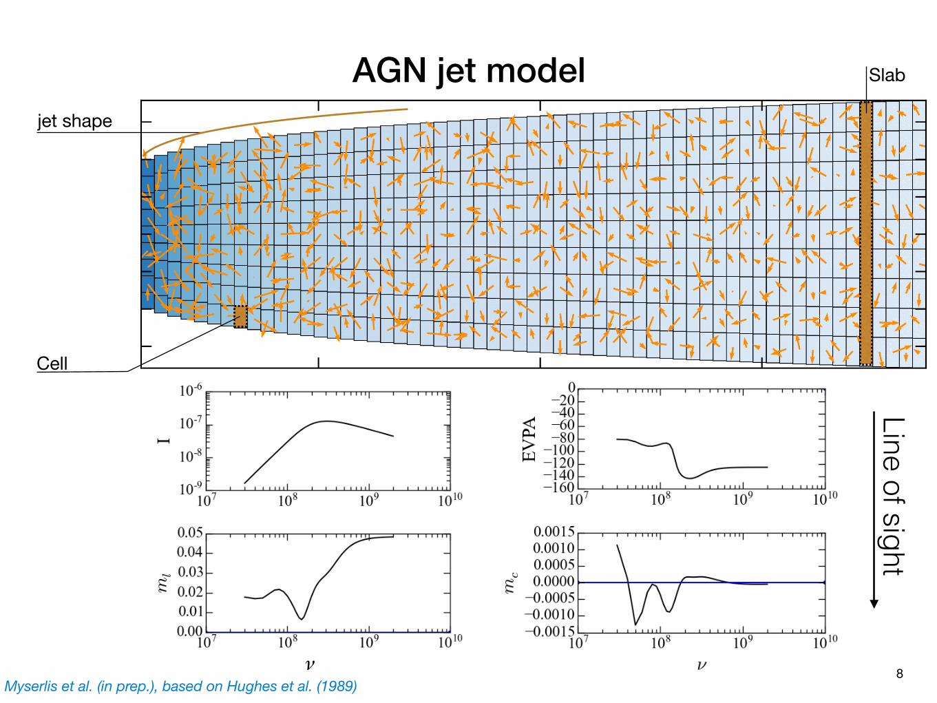
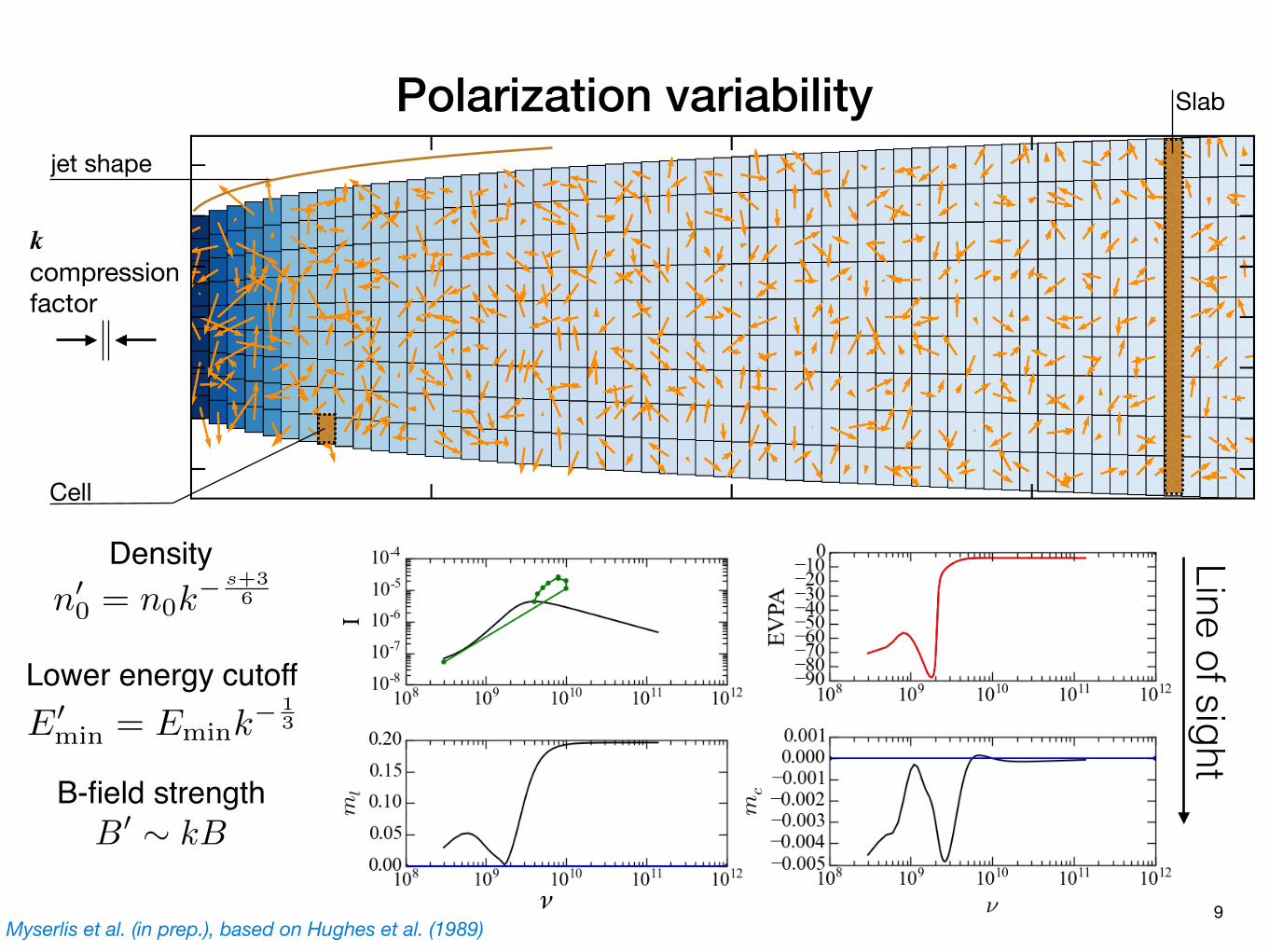
AGN jet modeljet shape

Line of sight

Cell

Slab

Myserlis et al. (in prep.), based on Hughes et al. (1989)8ν

ν

Polarization variabilityjet shape

Line of sight

Cell

n00 = n0k

� s+36

E0min = Emink

� 13

B0 ⇠ kB

Density

Lower energy cutoff

B-field strength

k compression factor

Slab

9Myserlis et al. (in prep.), based on Hughes et al. (1989)

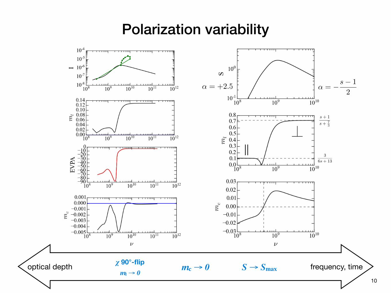
10

frequency, timeoptical depth S → Smaxmc → 0χ 90°-flip ml → 0

s+ 1

s+ 73

3

6s+ 13

↵ = �s� 1

2

||⏊

↵ = +2.5

Polarization variability

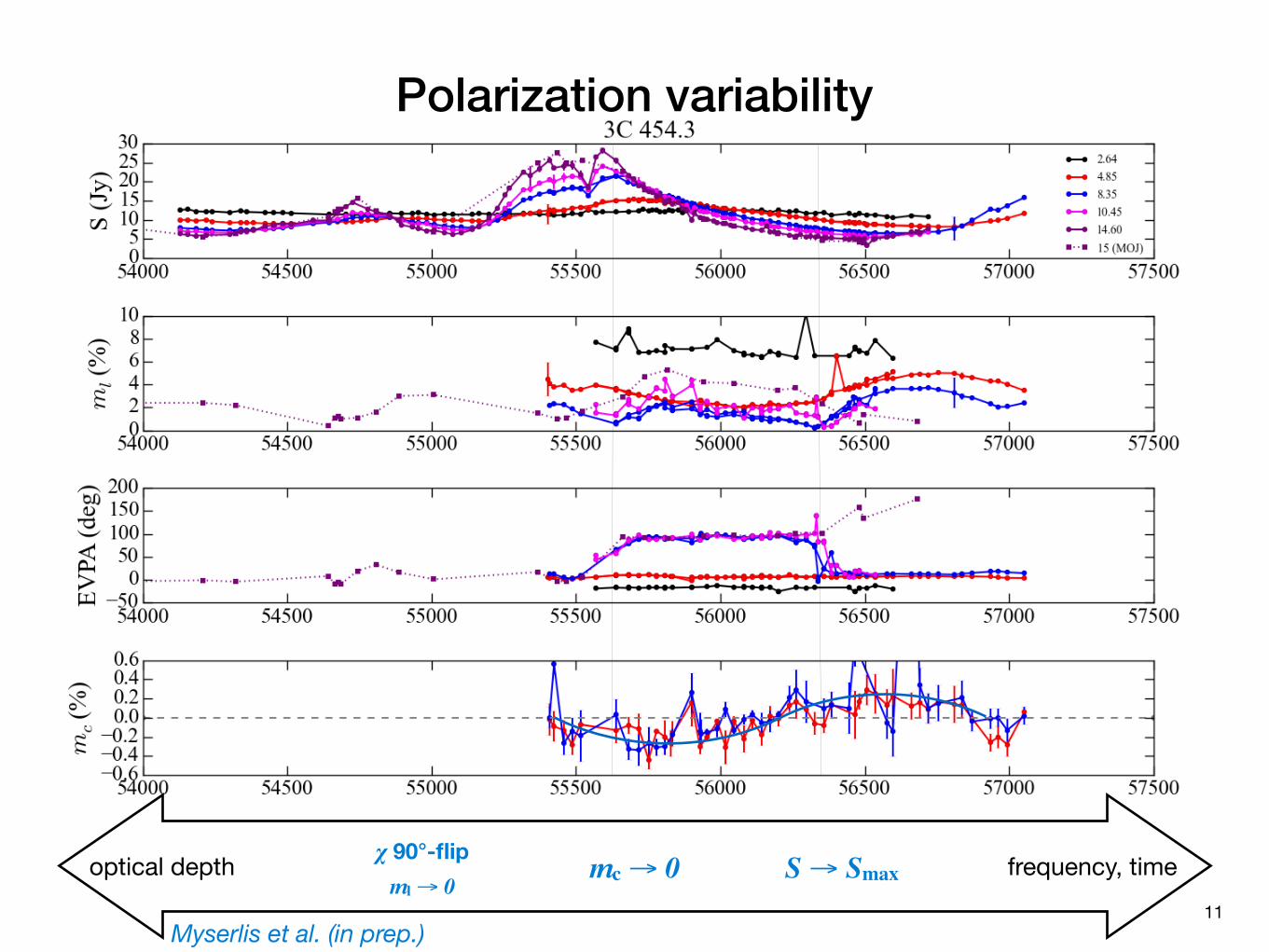
11Myserlis et al. (in prep.)

frequency, timeoptical depth S → Smaxmc → 0χ 90°-flip ml → 0

Polarization variability

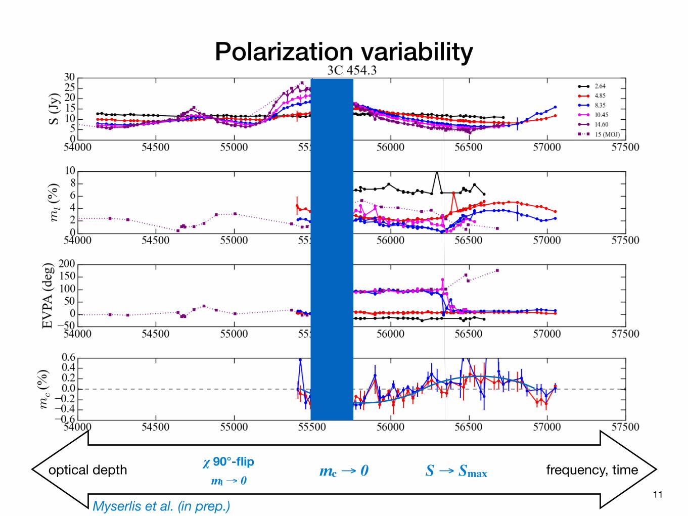
11Myserlis et al. (in prep.)

frequency, timeoptical depth S → Smaxmc → 0χ 90°-flip ml → 0

Polarization variability

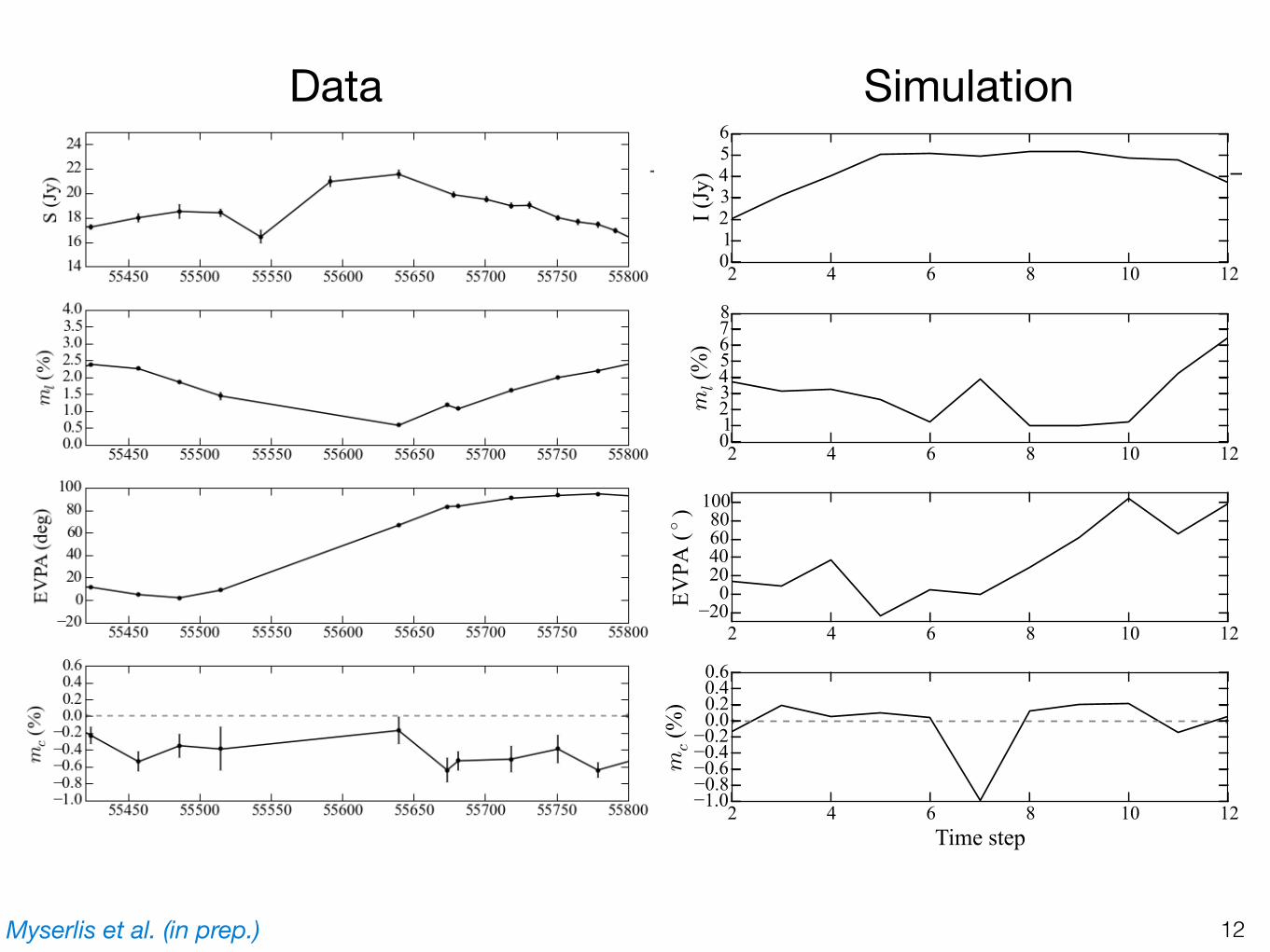
5.4. A STUDY CASE: THE BLAZAR 3C454.3 117

Figure 5.9: Simulated Full Stokes lightcurves as generated with our computer code.

since we observe a 90◦ rotation of the EVPA, concurrent with a minimization of the linearpolarization degree, ml. The corresponding change in handedness for the circular polarizationis also observed in the specific example, although the dataset is very noisy and the circularpolarization degree remains in general very low.

In conclusion, we believe that the computer code we developed is a powerful tool for theinvestigation of the physical characteristics of AGN jets. The combination of total flux andpolarization information we observe puts strict constrains on the parameters of the code whichin turn can be used directly to extract information for the shock compression factor, Dopplerfactor and the density of the shocked material. Furthermore, the code can be used to study theinfluence of Faraday effects on the emitted radiation since these radiative transfer parametersare coded at its core. Finally, this framework can be enriched by useful modifications, likethe addition of the lepton number which is discussed in subsection 4.4.3, which can be usedto answer fundamental open questions of AGN jets like their composition (electron–proton orelectron–positron).

Data Simulation5.4.ASTUDYCASE:THEBLAZAR3C454.3117

Figure5.9:SimulatedFullStokeslightcurvesasgeneratedwithourcomputercode.

sinceweobservea90◦rotationoftheEVPA,concurrentwithaminimizationofthelinearpolarizationdegree,ml.Thecorrespondingchangeinhandednessforthecircularpolarizationisalsoobservedinthespecificexample,althoughthedatasetisverynoisyandthecircularpolarizationdegreeremainsingeneralverylow.

Inconclusion,webelievethatthecomputercodewedevelopedisapowerfultoolfortheinvestigationofthephysicalcharacteristicsofAGNjets.Thecombinationoftotalfluxandpolarizationinformationweobserveputsstrictconstrainsontheparametersofthecodewhichinturncanbeuseddirectlytoextractinformationfortheshockcompressionfactor,Dopplerfactorandthedensityoftheshockedmaterial.Furthermore,thecodecanbeusedtostudytheinfluenceofFaradayeffectsontheemittedradiationsincetheseradiativetransferparametersarecodedatitscore.Finally,thisframeworkcanbeenrichedbyusefulmodifications,liketheadditionoftheleptonnumberwhichisdiscussedinsubsection4.4.3,whichcanbeusedtoanswerfundamentalopenquestionsofAGNjetsliketheircomposition(electron–protonorelectron–positron).

Myserlis et al. (in prep.) 12

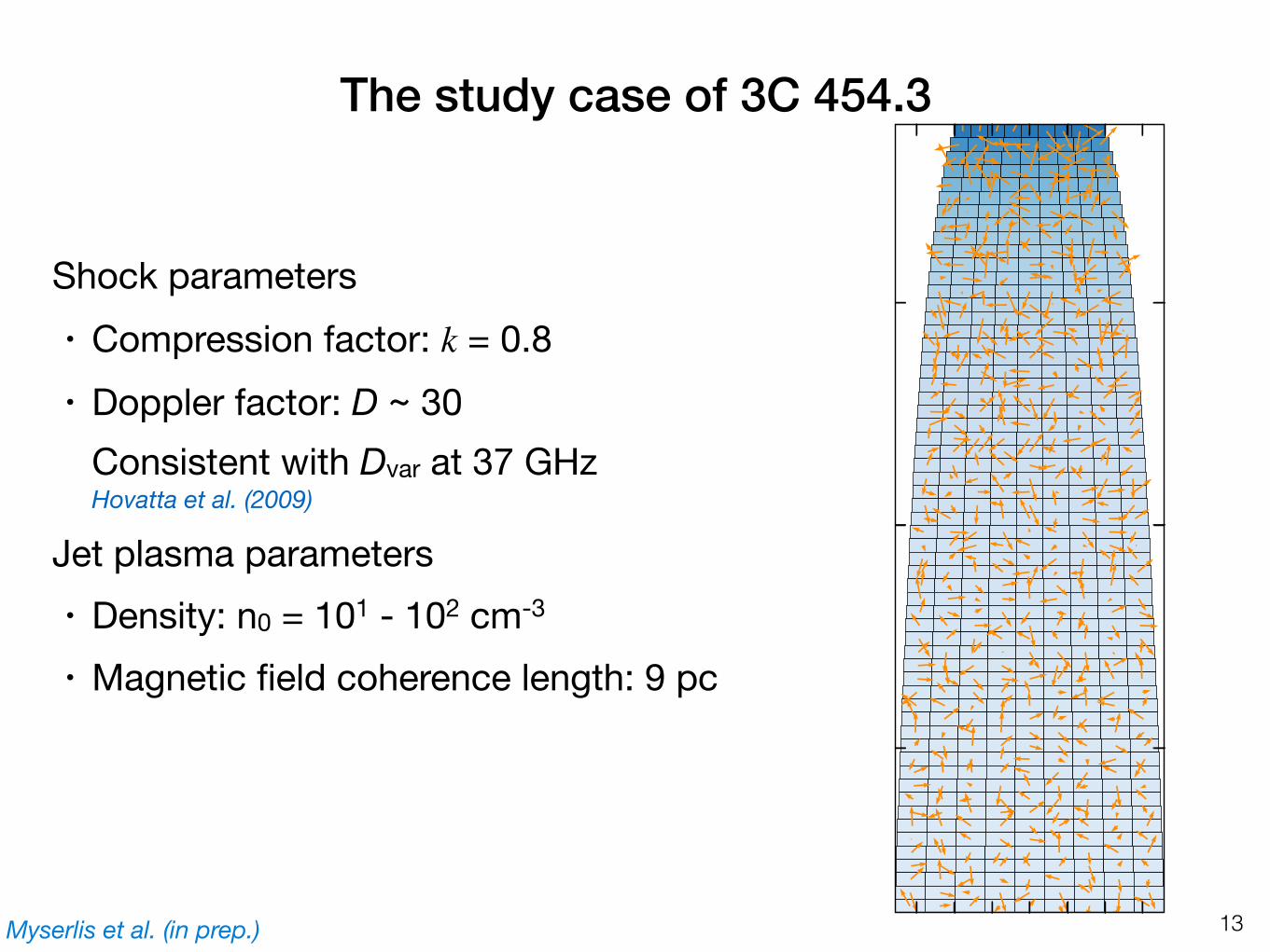
Shock parameters• Compression factor: k = 0.8• Doppler factor: D ~ 30

Consistent with Dvar at 37 GHzHovatta et al. (2009)

Jet plasma parameters• Density: n0 = 101 - 102 cm-3• Magnetic field coherence length: 9 pc

Myserlis et al. (in prep.) 13

The study case of 3C 454.3

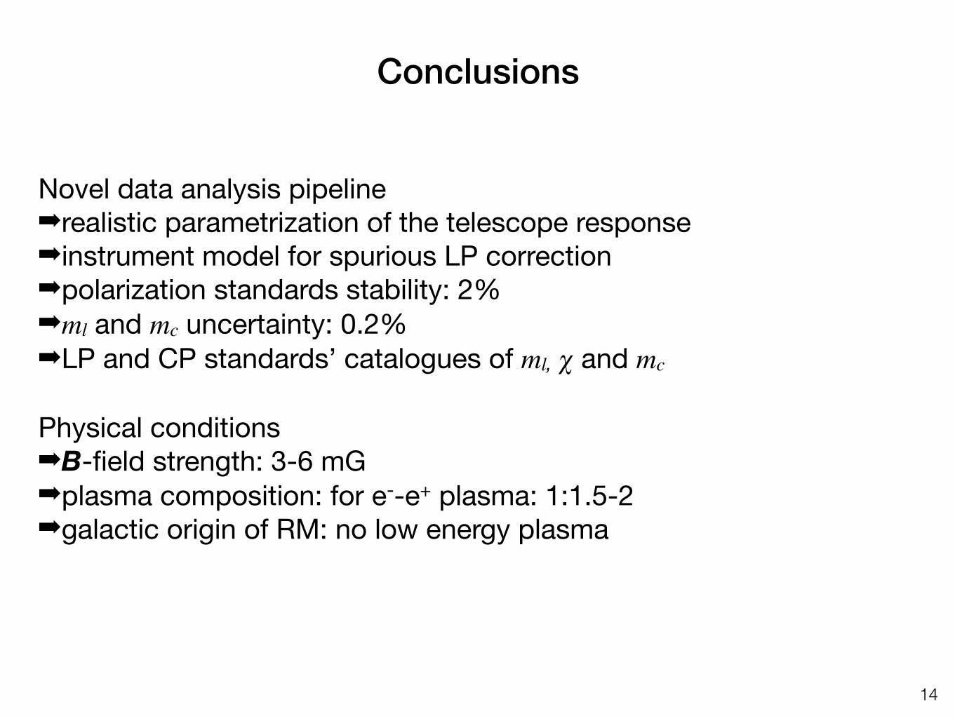
Novel data analysis pipeline➡realistic parametrization of the telescope response ➡instrument model for spurious LP correction➡polarization standards stability: 2%➡ml and mc uncertainty: 0.2%➡LP and CP standards’ catalogues of ml, χ and mc

Physical conditions➡B-field strength: 3-6 mG➡plasma composition: for e--e+ plasma: 1:1.5-2➡galactic origin of RM: no low energy plasma

14

Conclusions

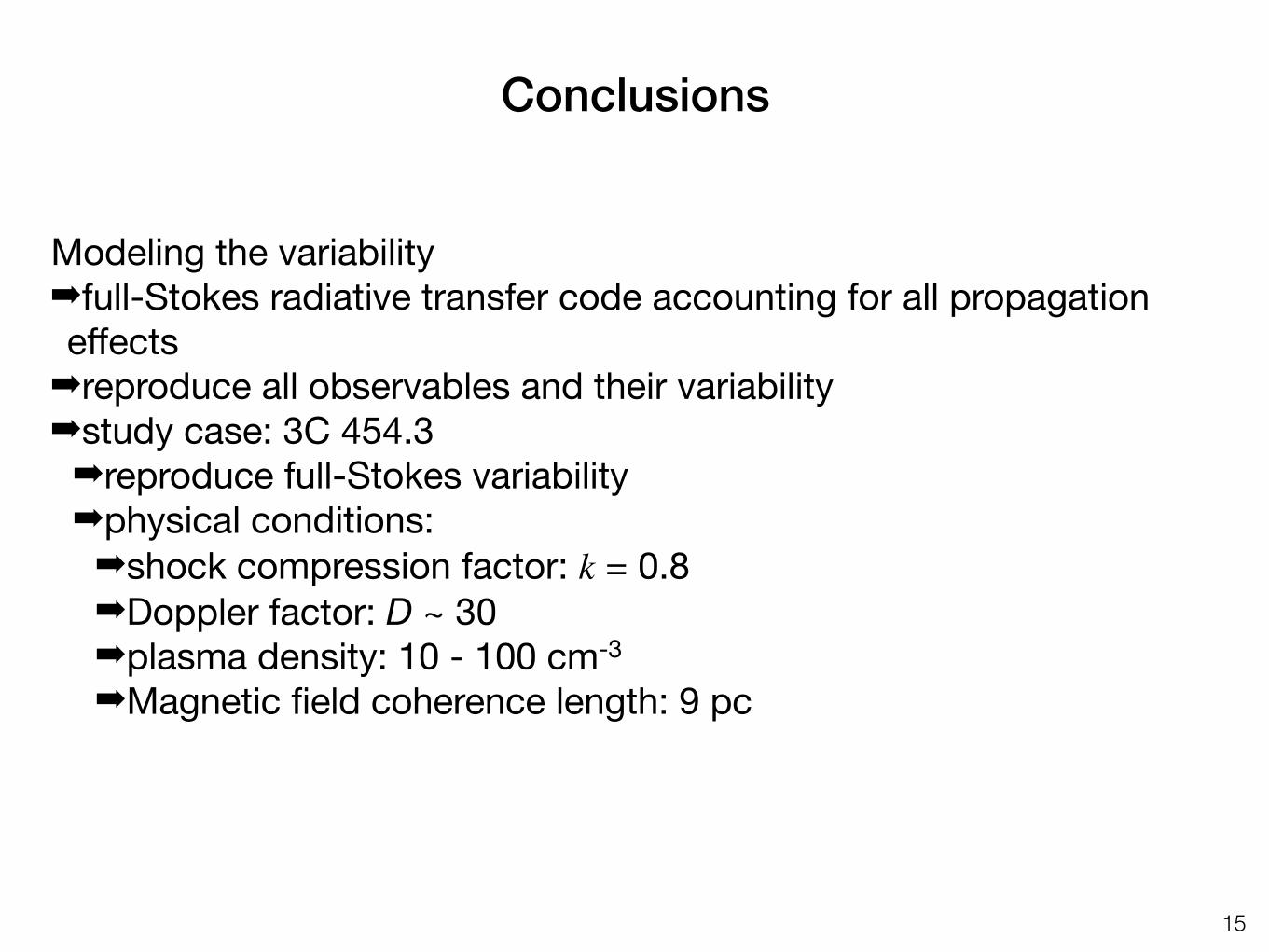
Modeling the variability➡full-Stokes radiative transfer code accounting for all propagation effects➡reproduce all observables and their variability➡study case: 3C 454.3➡reproduce full-Stokes variability➡physical conditions: ➡shock compression factor: k = 0.8➡Doppler factor: D ~ 30➡plasma density: 10 - 100 cm-3➡Magnetic field coherence length: 9 pc

15

Conclusions