Physics 403 - University of Rochester

Physics 403Maximum Likelihood and Least Squares II

Segev BenZvi

Department of Physics and AstronomyUniversity of Rochester

Table of Contents

1 Maximum LikelihoodProperties of ML EstimatorsVariances and the Minimum Variance BoundThe ∆ lnL = 1/2 RuleMaximum Likelihood in Several Dimensions

2 χ2 and the Method of Least SquaresGaussian and Poisson CasesFitting a Line to DataGeneralization to Correlated UncertaintiesNonlinear Least SquaresGoodness of Fit

Segev BenZvi (UR) PHY 403 2 / 32

Maximum Likelihood TechniqueI The method of maximum likelihood is an extremely important

technique used in frequentist statisticsI There is no mystery to it. Here is the connection to the Bayesian

view: given parameters x and data D, Bayes’ Theorem tells us that

p(x|D, I) ∝ p(D|x, I) p(x|I)

where we ignore the marginal evidence p(D|I)I Suppose p(x|I) = constant for all x. Then

p(x|D, I) ∝ p(D|x, I)

and the best estimator x is simply the value that maximizes thelikelihood p(D|x, I)

I So the method of maximum likelihood for a frequentist isequivalent to maximizing the posterior p(x|D, I) with uniformpriors on the {xi}.Segev BenZvi (UR) PHY 403 3 / 32

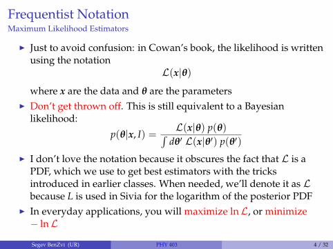
Frequentist NotationMaximum Likelihood Estimators

I Just to avoid confusion: in Cowan’s book, the likelihood is writtenusing the notation

L(x|θ)where x are the data and θ are the parameters

I Don’t get thrown off. This is still equivalent to a Bayesianlikelihood:

p(θ|x, I) =L(x|θ) p(θ)∫

dθ′ L(x|θ′) p(θ′)

I I don’t love the notation because it obscures the fact that L is aPDF, which we use to get best estimators with the tricksintroduced in earlier classes. When needed, we’ll denote it as Lbecause L is used in Sivia for the logarithm of the posterior PDF

I In everyday applications, you will maximize lnL, or minimize− lnLSegev BenZvi (UR) PHY 403 4 / 32

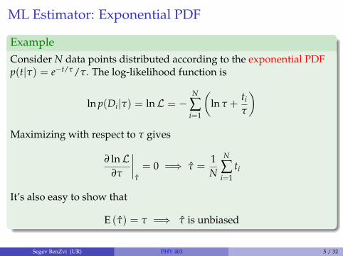
ML Estimator: Exponential PDF

ExampleConsider N data points distributed according to the exponential PDFp(t|τ) = e−t/τ/τ. The log-likelihood function is

ln p(Di|τ) = lnL = −N

∑i=1

(ln τ +

ti

τ

)Maximizing with respect to τ gives

∂ lnL∂τ

∣∣∣∣τ

= 0 =⇒ τ =1N

N

∑i=1

ti

It’s also easy to show that

E (τ) = τ =⇒ τ is unbiased


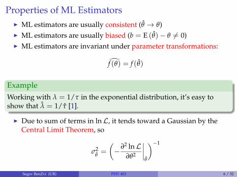
Properties of ML EstimatorsI ML estimators are usually consistent (θ → θ)I ML estimators are usually biased (b = E (θ)− θ 6= 0)I ML estimators are invariant under parameter transformations:

f (θ) = f (θ)

ExampleWorking with λ = 1/τ in the exponential distribution, it’s easy toshow that λ = 1/τ [1].

I Due to sum of terms in lnL, it tends toward a Gaussian by theCentral Limit Theorem, so

σ2θ=

(−∂2 lnL

∂θ2

∣∣∣∣θ

)−1


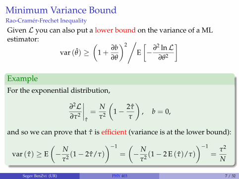
Minimum Variance BoundRao-Cramér-Frechet Inequality

Given L you can also put a lower bound on the variance of a MLestimator:

var (θ) ≥(

1 +∂b∂θ

)2/

E[−∂2 lnL

∂θ2

]

ExampleFor the exponential distribution,

∂2L∂τ2

∣∣∣∣τ

=Nτ2

(1− 2τ

τ

), b = 0,

and so we can prove that τ is efficient (variance is at the lower bound):

var (τ) ≥ E(−N

τ2 (1− 2τ/τ)

)−1

=

(−N

τ2 (1− 2 E (τ)/τ)

)−1

=τ2

N


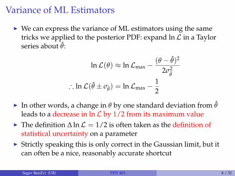
Variance of ML Estimators

I We can express the variance of ML estimators using the sametricks we applied to the posterior PDF: expand lnL in a Taylorseries about θ:

lnL(θ) ≈ lnLmax −(θ − θ)2

2σ2θ

∴ lnL(θ ± σθ) = lnLmax −12

I In other words, a change in θ by one standard deviation from θleads to a decrease in lnL by 1/2 from its maximum value

I The definition ∆ lnL = 1/2 is often taken as the definition ofstatistical uncertainty on a parameter

I Strictly speaking this is only correct in the Gaussian limit, but itcan often be a nice, reasonably accurate shortcut


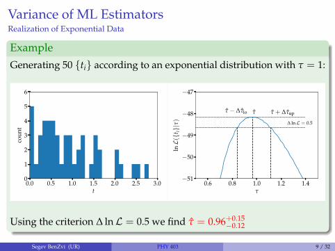
Variance of ML EstimatorsRealization of Exponential Data

Example

Generating 50 {ti} according to an exponential distribution with τ = 1:

0.0 0.5 1.0 1.5 2.0 2.5 3.0t

0

1

2

3

4

5

6

coun

t

0.6 0.8 1.0 1.2 1.4τ

−51

−50

−49

−48

−47

lnL({t

i}|τ

)

ττ − ∆τlo τ + ∆τup

∆ lnL = 0.5

Using the criterion ∆ lnL = 0.5 we find τ = 0.96+0.15−0.12


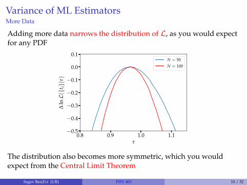
Variance of ML EstimatorsMore Data

Adding more data narrows the distribution of L, as you would expectfor any PDF

0.8 0.9 1.0 1.1τ

−0.5

−0.4

−0.3

−0.2

−0.1

0.0

0.1∆

lnL({t

i}|τ

)N = 50N = 100

The distribution also becomes more symmetric, which you wouldexpect from the Central Limit Theorem


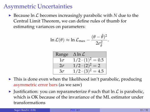
Asymmetric UncertaintiesI Because lnL becomes increasingly parabolic with N due to the

Central Limit Theorem, we can define rules of thumb forestimating variances on parameters:

lnL(θ) ≈ lnLmax −(θ − θ)2

2σ2θ

.

Range ∆ lnL1σ 1/2 · (1)2 = 0.52σ 1/2 · (2)2 = 23σ 1/2 · (3)2 = 4.5

I This is done even when the likelihood isn’t parabolic, producingasymmetric error bars (as we saw)

I Justification: you can reparameterize θ such that lnL is parabolic,which is OK because of the invariance of the ML estimator undertransformationsSegev BenZvi (UR) PHY 403 11 / 32

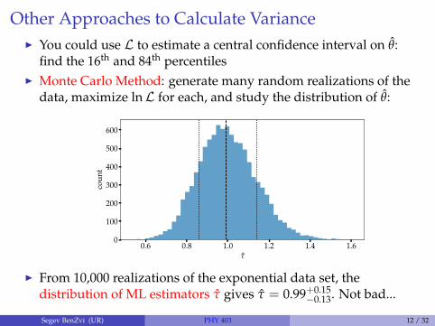
Other Approaches to Calculate VarianceI You could use L to estimate a central confidence interval on θ:

find the 16th and 84th percentilesI Monte Carlo Method: generate many random realizations of the

data, maximize lnL for each, and study the distribution of θ:

0.6 0.8 1.0 1.2 1.4 1.6τ

0

100

200

300

400

500

600

coun

t

I From 10,000 realizations of the exponential data set, thedistribution of ML estimators τ gives τ = 0.99+0.15

−0.13. Not bad...


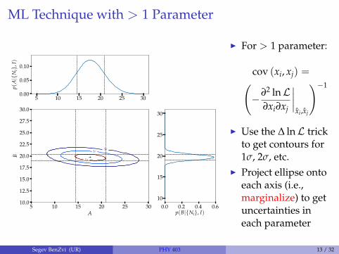
ML Technique with > 1 Parameter

5 10 15 20 25 300.00

0.05

0.10

p(A|{

Ni},

I)

5 10 15 20 25 30A

10.0

12.5

15.0

17.5

20.0

22.5

25.0

27.5

30.0

B

3σ2σ

1σ

0.0 0.2 0.4 0.6p(B|{Ni}, I)

10

15

20

25

30

I For > 1 parameter:

cov (xi, xj) =(−∂2 lnL

∂xi∂xj

∣∣∣∣xi,xj

)−1

I Use the ∆ lnL trickto get contours for1σ, 2σ, etc.

I Project ellipse ontoeach axis (i.e.,marginalize) to getuncertainties ineach parameter


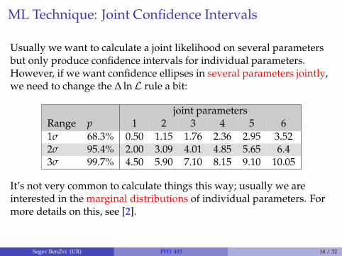
ML Technique: Joint Confidence Intervals

Usually we want to calculate a joint likelihood on several parametersbut only produce confidence intervals for individual parameters.However, if we want confidence ellipses in several parameters jointly,we need to change the ∆ lnL rule a bit:

joint parametersRange p 1 2 3 4 5 61σ 68.3% 0.50 1.15 1.76 2.36 2.95 3.522σ 95.4% 2.00 3.09 4.01 4.85 5.65 6.43σ 99.7% 4.50 5.90 7.10 8.15 9.10 10.05

It’s not very common to calculate things this way; usually we areinterested in the marginal distributions of individual parameters. Formore details on this, see [2].


Table of Contents

1 Maximum LikelihoodProperties of ML EstimatorsVariances and the Minimum Variance BoundThe ∆ lnL = 1/2 RuleMaximum Likelihood in Several Dimensions

2 χ2 and the Method of Least SquaresGaussian and Poisson CasesFitting a Line to DataGeneralization to Correlated UncertaintiesNonlinear Least SquaresGoodness of Fit


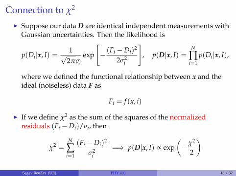
Connection to χ2

I Suppose our data D are identical independent measurements withGaussian uncertainties. Then the likelihood is

p(Di|x, I) =1√

2πσiexp

[− (Fi −Di)

2

2σ2i

], p(D|x, I) =

N

∏i=1

p(Di|x, I),

where we defined the functional relationship between x and theideal (noiseless) data F as

Fi = f (x, i)

I If we define χ2 as the sum of the squares of the normalizedresiduals (Fi −Di)/σi, then

χ2 =N

∑i=1

(Fi −Di)2

σ2i

=⇒ p(D|x, I) ∝ exp(−χ2

2

)


Maximum Likelihood and Least Squares

I With a uniform prior on x, the logarithm of the posterior PDF is

L = ln p(x|D, I) = ln p(D|x, I) = constant− χ2

2

I The maximum of the posterior (and likelihood) will occur whenχ2 is a minimum. Hence, the optimal solution x is called the leastsquares estimate

I Least squares/maximum likelihood is used all the time in dataanalysis, but...

I Note: there is nothing mysterious or even fundamental about this;least squares is what Bayes’ Theorem reduces to if:

1. Your prior on your parameters is uniform2. The uncertainties on your data are Gaussian


Maximum Likelihood: Poisson CaseI Suppose that our data aren’t Gaussian, but a set of Poisson counts

n with expectation values ν. E.g., we are dealing with binned datain a histogram. Then the likelihood becomes

p(n|ν, I) =N

∏i=1

νnii e−νi

ni!

I In the limit N → large, this becomes

p(ni|νi, I) ∝ exp

[−

N

∑i=1

(ni − νi)2

2νi

]

I The corresponding χ2 statistic is given by

χ2 =N

∑i=1

(ni − νi)2

νi


Pearson’s χ2 Test

I The quantity

χ2 =N

∑i=1

(ni − νi)2

νi

is also known as Pearson’s χ2 statisticI Pearson’s χ2 test is a standard frequentist method for comparing

histogrammed counts {ni} against a theoretical expectation {νi}I Convenient property: this test statistic will be asymptotically

distributed like χ2N regardless of the actual distribution that

generates the relative counts {ni}. It is distribution freeI In practice, we can use Pearson’s χ2 to calculate a p-value

p(χ2Pearson ≥ χ2|N)

I Caveat: the counts in each bin must not be too small; ni ≥ 5 for alli is a reasonable rule of thumb


Modified Least Squares

0 2 4 6 8 10x

0.00

0.05

0.10

0.15

0.20

0.25

coun

t

f (x)

data

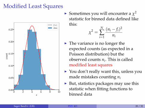
I Sometimes you will encounter a χ2

statistic for binned data defined likethis:

χ2 =N

∑i=1

(ni − fi)2

ni

I The variance is no longer theexpected counts (as expected in aPoisson distribution) but theobserved counts ni. This is calledmodified least squares

I You don’t really want this, unless youmade mistakes counting ni

I But, statistics packages may use thisstatistic when fitting functions tobinned data


Robustness of Least Squares Algorithm

I Our definition of χ2 as the quadrature sum (or l2-norm) of theresiduals makes a lot of calculations easy, but it isn’t particularlyrobust. I.e., it can be affected by outliers

I Note: the l1-norm

l1-norm =N

∑i=1

∣∣∣∣Fi −Di

σi

∣∣∣∣is much more robust against outliers in the data

I This isn’t used too often but if your function f (x) is linear in theparameters it’s not hard to calculate

I See chapter 15 of Numerical Recipes in C for an implementation[2]

I In Python there should be an implementation in the statsmodelspackage [3]


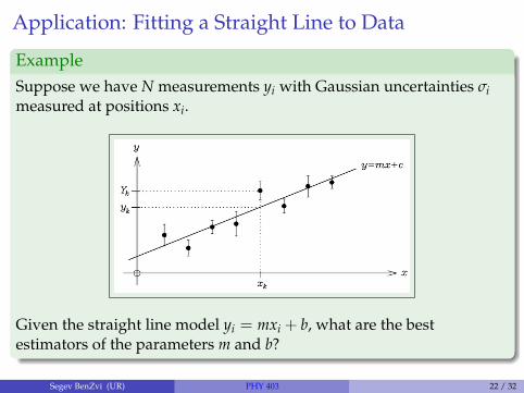
Application: Fitting a Straight Line to Data

ExampleSuppose we have N measurements yi with Gaussian uncertainties σimeasured at positions xi.

Given the straight line model yi = mxi + b, what are the bestestimators of the parameters m and b?


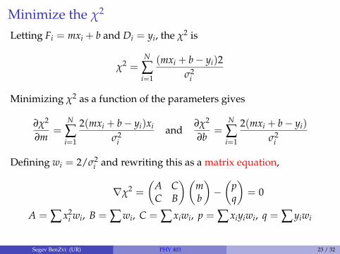
Minimize the χ2

Letting Fi = mxi + b and Di = yi, the χ2 is

χ2 =N

∑i=1

(mxi + b− yi)2σ2

i

Minimizing χ2 as a function of the parameters gives

∂χ2

∂m=

N

∑i=1

2(mxi + b− yi)xi

σ2i

and∂χ2

∂b=

N

∑i=1

2(mxi + b− yi)

σ2i

Defining wi = 2/σ2i and rewriting this as a matrix equation,

∇χ2 =

(A CC B

)(mb

)−(

pq

)= 0

A = ∑ x2i wi, B = ∑ wi, C = ∑ xiwi, p = ∑ xiyiwi, q = ∑ yiwi


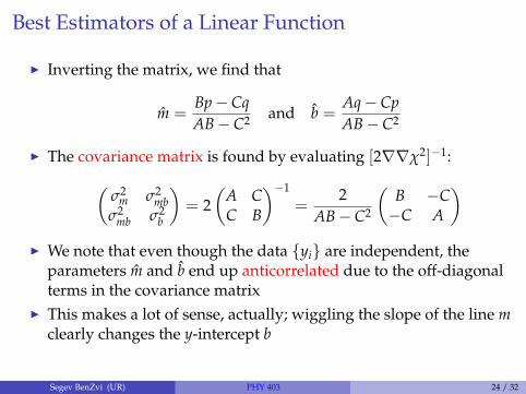
Best Estimators of a Linear Function

I Inverting the matrix, we find that

m =Bp− CqAB− C2 and b =

Aq− CpAB− C2

I The covariance matrix is found by evaluating [2∇∇χ2]−1:(σ2

m σ2mb

σ2mb σ2

b

)= 2

(A CC B

)−1

=2

AB− C2

(B −C−C A

)I We note that even though the data {yi} are independent, the

parameters m and b end up anticorrelated due to the off-diagonalterms in the covariance matrix

I This makes a lot of sense, actually; wiggling the slope of the line mclearly changes the y-intercept b


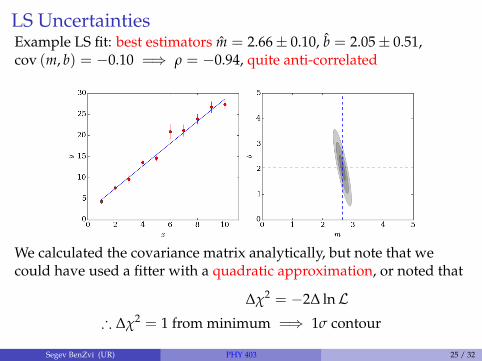
LS UncertaintiesExample LS fit: best estimators m = 2.66± 0.10, b = 2.05± 0.51,cov (m, b) = −0.10 =⇒ ρ = −0.94, quite anti-correlated

We calculated the covariance matrix analytically, but note that wecould have used a fitter with a quadratic approximation, or noted that

∆χ2 = −2∆ lnL∴ ∆χ2 = 1 from minimum =⇒ 1σ contour


Generalization: Correlated Uncertainties in DataI So far we have been focusing on the case where uncertainties in

our measurements are completely uncorrelatedI If this is not the case, then we can generalize χ2 to

χ2 =(y− y

)>σ−1 (y− y

)where σ is the covariance matrix of the data

I If the fit function depends linearly on the parameters,

y(x) =m

∑i=1

aifi(x), y = A · a, Aij = fj(xi)

then

χ2 =(y− y

)>σ−1 (y− y

)=(y−A · a

)>σ−1 (y−A · a

)Segev BenZvi (UR) PHY 403 26 / 32

Exact Solution to Linear Least Squares

I This is the case of linear least squares; the LS estimators of the {ai}are unbiased, efficient, and can be solved analytically

I The general solution:

χ2 =(y−A · a

)>σ−1 (y−A · a

)a = (A>σ−1A)−1A>σ−1 · y

cov (ai, aj) = (A>σ−1A)−1

I In practice one still minimizes numerically, because the matrixinversions in the analytical solution can be computationallyexpensive and numerically unstable

I Nice property: if uncertainties are Gaussian and the fit function islinear in the m parameters, then χ2 ∼ χ2

N−m. But often theseassumptions are broken, e.g., when using binned data with lowcounts


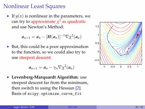
Nonlinear Least Squares

I If y(x) is nonlinear in the parameters, wecan try to approximate χ2 as quadraticand use Newton’s Method:

an+1 = an − [H(an)]−1∇χ2(an)

I But, this could be a poor approximationto the function, so we could also try touse steepest descent:

an+1 = an − γn∇χ2(an)

I Levenberg-Marquardt Algorithm: usesteepest descent far from the minimum,then switch to using the Hessian [2].Basis of scipy.optimize.curve_fit


χ2 and Goodness of Fit

I Because χ2 ∼ χ2N−m if several conditions are satisfied, it can be

used to estimate the goodness of fitI Basic idea: the outcome of Linear Least Squares is the value χ2

min.Goodness of fit comes from calculating the p-value

p(χ2 ≥ χ2min|N, m)

I This tail probability tells us how unlikely it is to have observedour data given the model and its best fit parameters

I Recall the warning about p-values: they are biased against the nullhypothesis that the model is correct, and can lead you tospuriously reject a model

I The 5σ rule applies, because we’re not dealing with a properposterior PDF


ML and Goodness of Fit

I The ML technique does not provide a similar goodness of fitparameter because there is no standard reference distribution tocompare to

I Suggested approach: estimate paramaters with ML, but calculategoodness of fit by binning the data and using χ2

I Note: be careful about assuming that your χ2 statistic actuallyfollows a χ2 distribution. Remember that this is true only forlinear models with Gaussian uncertainties

I This isn’t the 1920s. Use simulation to model the distribution ofyour χ2 statistic and calculate p-values from that distribution


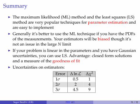
Summary

I The maximum likelihood (ML) method and the least squares (LS)method are very popular techniques for parameter estimation andare easy to implement

I Generally it’s better to use the ML technique if you have the PDFsof the measurements. Your estimators will be biased though it’snot an issue in the large N limit

I If your problem is linear in the parameters and you have Gaussianuncertainties, you can use LS. Advantage: closed form solutionsand a measure of the goodness of fit

I Uncertainties on estimators:

Error ∆ lnL ∆χ2

1σ 0.5 12σ 2 43σ 4.5 9


References I

[1] Glen Cowan. Statistical Data Analysis. New York: OxfordUniversity Press, 1998.

[2] W. Press et al. Numerical Recipes in C. New York: CambridgeUniversity Press, 1992. URL: http://www.nr.com.

[3] Statsmodels. URL: http://statsmodels.sourceforge.net/.


http://www.nr.com

http://statsmodels.sourceforge.net/

Physics 403 - University of Rochester

Documents

Transcript of Physics 403 - University of Rochester