Physics 215c: Problem Set 4

Prof. Matthew Fisher

Solutions prepared by: James Sully

June 20, 2013

Please let me know if you encounter any typos in the solutions.

Problem 1 (25)

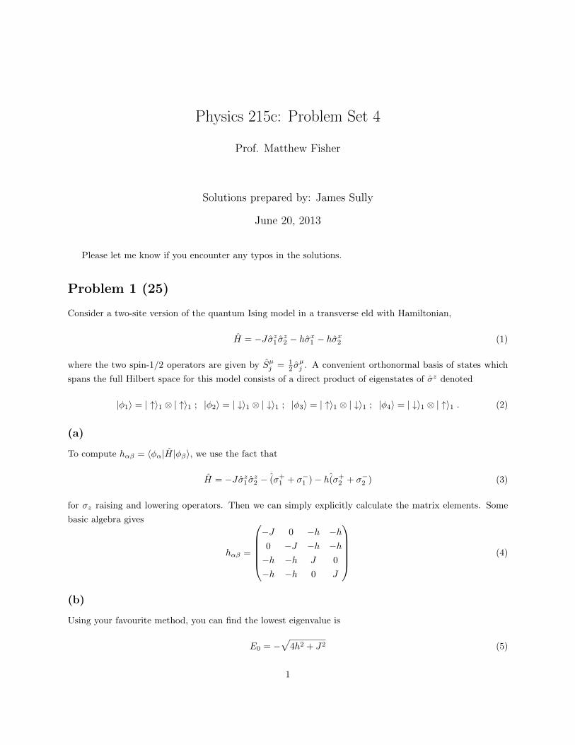
Consider a two-site version of the quantum Ising model in a transverse eld with Hamiltonian,

H = −Jσz1 σz2 − hσx1 − hσx2 (1)

where the two spin-1/2 operators are given by Sµj = 12 σ

µj . A convenient orthonormal basis of states which

spans the full Hilbert space for this model consists of a direct product of eigenstates of σz denoted

|φ1〉 = | ↑〉1 ⊗ | ↑〉1 ; |φ2〉 = | ↓〉1 ⊗ | ↓〉1 ; |φ3〉 = | ↑〉1 ⊗ | ↓〉1 ; |φ4〉 = | ↓〉1 ⊗ | ↑〉1 . (2)

(a)

To compute hαβ = 〈φα|H|φβ〉, we use the fact that

H = −Jσz1 σz2 − (σ+1 + σ−1 )− h(σ+

2 + σ−2 ) (3)

for σz raising and lowering operators. Then we can simply explicitly calculate the matrix elements. Some

basic algebra gives

hαβ =

−J 0 −h −h0 −J −h −h−h −h J 0

−h −h 0 J

(4)

(b)

Using your favourite method, you can find the lowest eigenvalue is

E0 = −√

4h2 + J2 (5)

1

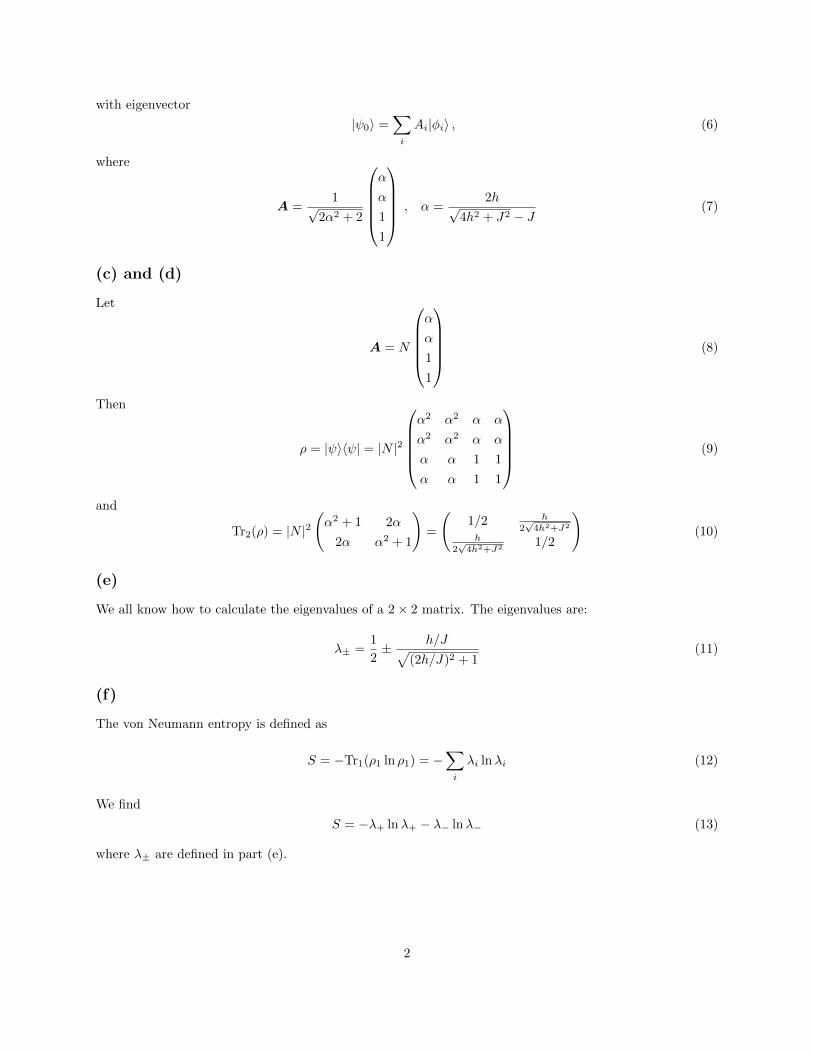
with eigenvector

|ψ0〉 =∑i

Ai|φi〉 , (6)

where

A =1√

2α2 + 2

α

α

1

1

, α =2h√

4h2 + J2 − J(7)

(c) and (d)

Let

A = N

α

α

1

1

(8)

Then

ρ = |ψ〉〈ψ| = |N |2

α2 α2 α α

α2 α2 α α

α α 1 1

α α 1 1

(9)

and

Tr2(ρ) = |N |2(α2 + 1 2α

2α α2 + 1

)=

(1/2 h

2√4h2+J2

h2√4h2+J2

1/2

)(10)

(e)

We all know how to calculate the eigenvalues of a 2× 2 matrix. The eigenvalues are:

λ± =1

2± h/J√

(2h/J)2 + 1(11)

(f)

The von Neumann entropy is defined as

S = −Tr1(ρ1 ln ρ1) = −∑i

λi lnλi (12)

We find

S = −λ+ lnλ+ − λ− lnλ− (13)

where λ± are defined in part (e).

2

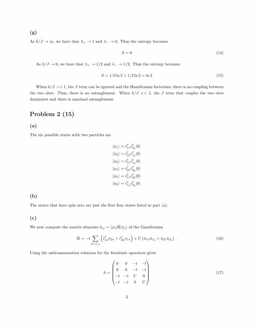
(g)

As h/J →∞, we have that λ+ → 1 and λ− → 0. Thus the entropy becomes

S = 0 (14)

As h/J → 0, we have that λ+ → 1/2 and λ− → 1/2. Thus the entropy becomes

S = 1/2 ln 2 + 1/2 ln 2 = ln 2 (15)

When h/J >> 1, the J term can be ignored and the Hamiltonian factorizes; there is no coupling between

the two sites. Thus, there is no entanglement. When h/J << 1, the J term that couples the two sites

dominates and there is maximal entanglement.

Problem 2 (15)

(a)

The six possible states with two particles are

|φ1〉 = c†1↑c†2↓|0〉

|φ2〉 = c†2↑c†1↓|0〉

|φ3〉 = c†1↑c†1↓|0〉

|φ4〉 = c†2↑c†2↓|0〉

|φ5〉 = c†1↑c†2↑|0〉

|φ6〉 = c†1↓c†2↓|0〉

(b)

The states that have spin zero are just the first four states listed in part (a).

(c)

We now compute the matrix elements hij = 〈φi|H|φj〉 of the Gamiltonian

H = −t∑σ=↑,↓

(c†1σ c2σ + c†2σ c1σ

)+ U (n1↑n1↓ + n2↑n2↓) . (16)

Using the anticommutation relations for the fermionic operators gives

h =

0 0 −t −t0 0 −t −t−t −t U 0

−t −t 0 U

(17)

3

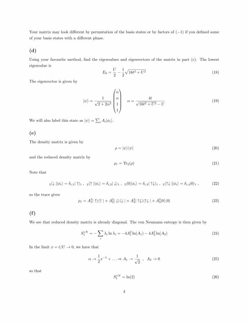
Your matrix may look different by perumtation of the basis states or by factors of (−1) if you defined some

of your basis states with a different phase.

(d)

Using your favourite method, find the eigenvalues and eigenvectors of the matrix in part (c). The lowest

eigenvalue is

E0 =U

2− 1

2

√16t2 + U2 (18)

The eigenvector is given by

|ψ〉 =1√

2 + 2α2

α

α

1

1

α =4t√

16t2 + U2 − U(19)

We will also label this state as |ψ〉 =∑iAi|φi〉.

(e)

The density matrix is given by

ρ = |ψ〉〈ψ| (20)

and the reduced density matrix by

ρ1 = Tr2(ρ) (21)

Note that

2〈↓ ||φi〉 = δi,1| ↑〉1 , 2〈↑ ||φi〉 = δi,2| ↓〉1 , 2〈0||φi〉 = δi,3| ↑↓〉1 , 2〈↑↓ ||φi〉 = δi,4|0〉1 , (22)

so the trace gives

ρ1 = A21| ↑〉〈↑ |+A2

2| ↓〉〈↓ |+A23| ↑↓〉〈↑↓ |+A2

4|0〉〈0| (23)

(f)

We see that reduced density matrix is already diagonal. The von Neumann entropy is then given by

SvN1 = −∑i

λi lnλi = −4A21 ln(A1)− 4A2

3 ln(A3) (24)

In the limit x = t/U → 0, we have that

α→ 1

2x−1 + . . .⇒ A1 →

1√2, A3 → 0 (25)

so that

SvN1 = ln(2) (26)

4

We could have predicted this because the term that dominates is the one that couples the spins on the two

sites in a maximally entangled state.

Problem 3 (15)

(a)

Consider the inner product

〈n1, . . . , nN ||n′1, . . . , n′N 〉 (27)

Suppose there exists j such that nj 6= n′j . Then there is either a lone cj which annihilates the state to the

right (it anticommutes through all the other fermionic operators up to a factor of (−1)) or a lone c†j which

annihilates the state to the left in the same way. Thus theses states are orthogonal to each other.

To see they are normalized, we proceed as follows: let {nij}kj=1 be the set of non-zero ni. Then

〈n1, . . . , nN ||n1, . . . , nN 〉 = 〈0|cik . . . ci1c†i1. . . cik |0〉

= 〈0|cik . . . (1− c†i1ci1) . . . cik |0〉

= 〈0|cik . . . 1 . . . cik |0〉

(28)

Proceeding iteratively we find 〈n1, . . . , nN ||n1, . . . , nN 〉 = 1.

(b)

We have that

Hµ = |µ|N∑j=1

c†j cj = |µ|N∑j=1

nj (29)

where nj is the number operator. Thus

Hµ|n1, . . . , nN 〉 = |µ|N∑j=1

nj |n1, . . . , nN 〉 (30)

and so this is indeed an eigenstate.

(c)

The lowest energy state is just the state where all of the nj = 0. There is a unique such state. The first

excited states are thus with one nj = 1. There are N such states. The gap is |µ|.

5

(d)

We have

{γA,j , γA,j′} = −{c†j − cj , c†j′ − cj′}

= {cj , c†j′}+ {c†j , cj′}

= 2δjj′ (31)

and

{γB,j , γB,j′} = {c†j + cj , c†j′ + cj′}

= {cj , c†j′}+ {c†j , cj′}

= 2δjj′ (32)

and

{γA,j , γB,j′} = i{c†j − cj , c†j′ + cj′}

= −i{cj , c†j′}+ i{c†j , cj′}

= 0 (33)

(e)

We rewrite the Hamiltonian as

Ht = −t∑j

(c†jcj+1 − cjc†j+1 + cjcj+1 − c†jc

†j+1

)= −it

∑j

(c†j + cj

)(c†j+1 − cj+1

)= −it

∑j

γB,jγA,j+1 (34)

(f)

We rather mechanically check all of the cases:

{di, dj} =1

4{γA,i+1 + iγB,i, γA,j+1 + iγB,j}

=1

4{γA,i+1, γA,j+1} −

1

4{γB,i, γB,j}

=1

4(2δij − 2δij) = 0 (35)

6

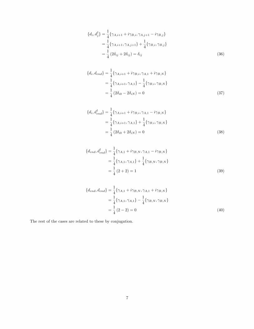
{di, d†j} =1

4{γA,i+1 + iγB,i, γA,j+1 − iγB,j}

=1

4{γA,i+1, γA,j+1}+

1

4{γB,i, γB,j}

=1

4(2δij + 2δij) = δij (36)

{di, dend} =1

4{γA,i+1 + iγB,i, γA,1 + iγB,N}

=1

4{γA,i+1, γA,1} −

1

4{γB,i, γB,N}

=1

4(2δi0 − 2δiN ) = 0 (37)

{di, d†end} =1

4{γA,i+1 + iγB,i, γA,1 − iγB,N}

=1

4{γA,i+1, γA,1}+

1

4{γB,i, γB,N}

=1

4(2δi0 + 2δiN ) = 0 (38)

{dend, d†end} =1

4{γA,1 + iγB,N , γA,1 − iγB,N}

=1

4{γA,1, γA,1}+

1

4{γB,N , γB,N}

=1

4(2 + 2) = 1 (39)

{dend, dend} =1

4{γA,1 + iγB,N , γA,1 + iγB,N}

=1

4{γA,1, γA,1} −

1

4{γB,N , γB,N}

=1

4(2− 2) = 0 (40)

The rest of the cases are related to these by conjugation.

7

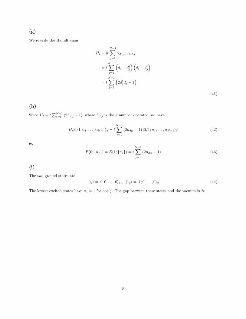
(g)

We rewrite the Hamiltonian

Ht = it

N−1∑j=1

γA,j+1γB,j

= t

N−1∑j=1

(dj + d†j

)(dj − d†j

)

= t

N−1∑j=1

(2d†jdj − 1

)(41)

(h)

Since Ht = t∑N−1j=1 (2nd;j − 1), where nd;j is the d number operator, we have

Ht|0/1;n1, . . . , nN−1〉d = t

N−1∑j=1

(2nd;j − 1) |0/1;n1, . . . , nN−1〉d (42)

ie,

E(0; {nj}) = E(1; {nj}) = t

N−1∑j=1

(2nd;j − 1) (43)

(i)

The two ground states are

|0g〉 = |0; 0, . . . , 0〉d , |1g〉 = |1; 0, . . . , 0〉d (44)

The lowest excited states have nj = 1 for one j. The gap between these states and the vacuum is 2t.

8