Phase Synchronization

Lecture by: Zhibin GuoNotes by: Xiang Fan

May 10, 2016

1 Introduction

For any mode or fluctuation, we always have

ϕk = |ϕk(x, t)|eiS(x,t) (1)

where S(x, t) is phase.If a mode amplitude satisfies

|ϕk(x, t)| ∝ eγt (2)

and γ → 0, we call it the marginal state. Near the marginal state, we have

∂tϕk ∼ ∂teiS(x,t) ∼ ∂tS(x, t) (3)

This means near the marginal state, the evolution of the mode is essentiallydetermined by its phase. That’s why phase dynamics matters!

References are listed in the end of this note.This lecture will cover the following two topics:

• A nonlinear Limit-Cycle-Oscillator (LCO) – Stuart-Landau Equation

• Collective behavior of many LCOs – Kuramoto Model

1

2 A Self Interacted LCO: Autonomous Sys-

tem

In this section, we study an autonomous system that satisfy the followingfirst order differential equation:

d

dtX = F (X;µ) (4)

where X = (X1, X2, ..., Xn) is a vector, µ means the scalar parameters inthis system. Eq. (4) is a very general form, many specific systems can bewritten in the above form. Examples of µ: it can be temperature, density orgradients of them in plasma physics.

For some range of µ, the system may stay stable; when µ exceeds somecritical value µc, the system may give a periodic motion solution. The criticalpoint where a system’s stability switches and a periodic solution arises iscalled the Hopf bifurcation.

• µ < µc: The system stays in a fixed or stationary state.

• µ > µc: The oscillator evolves into LCO state.

An example: simple harmonic oscillator:

d

dtx = v (5)

d

dtv = −kx (6)

Here X1 is x and X2 is v, the scalar parameter µ is k. The critical value iskc = 0: when k = 0 the system is stationary and when k > 0 the solution isperiodic motion.

Let X0(µ) denote a steady solution of Eq. (4), i.e. F (X0(µ);µ) = 0.Note that there is always a stationary solution, the question is whether thissolution is stable. We express Eq. (4) in terms of the deviation u = X−X0

in a Taylor series:

d

dtu = Lu+Muu+Nuuu+ ... (7)

2

where

(Lu)i =∑j

∂Fi(X0)∂X0j

uj (8)

(Muu)i =∑jk

12!

∂F 2i (X0)

∂X0j∂X0kujuk (9)

(Nuuu)i =∑jkl

13!

∂F 3i (X0)

∂X0j∂X0k∂X0lujukul (10)

2.1 Order by Order Expansion

Now assume µc = 0 for simplicity. Near criticality, suppose that µ is small,and do a reduced perturbation expansion:

L(µ) = L0 + µL1 + µ2L2 + ... (11)

It is convenient to define a small positive parameter ε by ε2χ = µ, whereχ = sgn(µ); ε is considered to be a measure of the amplitude to lowest order,so that one may assume the expansion:

u = εu1 + εu2 + ... (12)

Note that µ is ’equilibrium profile’ change, so it is smaller than the fluctuationamplitude change, that’s why µ is assumed to be of order ε2. Thus Eq. (11)now becomes

L = L0 + ε2χ2L1 + ε4L2 + ... (13)

Similarly,

M = M0 + ε2χ2M1 + ε4M2 + ... (14)

N = N0 + ε2χ2N1 + ε4N2 + ... (15)

All uν(t) (ν = 1, 2, ...) include fast and slow variations! We need to expandthe time coordinate, too. The slow variation is associated with profile change(related to µ), so it is plausible to assume

d

dt∼ ∂

∂t+ µ

∂

∂τ∼ ∂

∂t+ ε2

∂

∂τ(16)

3

Now we can expand L,M,N , u, and ddt, so we expand Eq. (7) order by

order:

ε1 : ( ∂∂t− L0)u1 = 0 (17)

ε2 : ( ∂∂t− L0)u2 = M0u1u1 (18)

ε3 : ( ∂∂t− L0)u3 = −(

∂

∂τ− χL1)u1 +N0u1u1u1 + 2M0u1u2 (19)

(20)

Generally,

(∂

∂t− L0)uν = Bν (21)

where

B1 = 0 (22)

B2 = M0u1u1 (23)

B3 = −( ∂∂τ

− χL1)u1 +N0u1u1u1 + 2M0u1u2 (24)

(25)

2.2 The solvability condition

L0 is the fast time scale. In order to remove the fast time scale, here weintroduce the left and right eigenvector:

L0U = λU (26)

U †L0 = λU † (27)

The first two eigenvalues can be expressed as λ0 = iω0 = U∗L0U , and λ1 =σ1 + iω1 = U ∗ L1U .

Multiply U † by Eq. (21), and we obtain the solvability condition:∫ 2π

0

U †(∂

∂t− L0)uνe

−iω0tdt =

∫ 2π

0

U †Bνe−iω0tdt = 0 (28)

Bν is 2π-periodic in ω0t, so we can express it in this form:

Bν(t, τ) =∞∑

l=−∞

B(l)ν (τ)eilω0t (29)

4

The solvability condition then becomes:

U †B(l)ν (τ) = 0 (30)

This condition is crucial.

2.3 Stuart-Landau Equation

For ν = 1, the solution for Eq. (21) has this form:

u1 = W (τ)Ueiω0t + c.c. (31)

where c.c. means complex conjugate, and W (τ) is some complex amplitudeyet to be solved. In order to obtain an equation for W , we need Eq. (30) forν = 2 and ν = 3.

For ν = 2, the Eq. (30) is trivially satisfied because U †U = 0.For ν = 3, express u2 in terms of u1 (or W ). u2 contains only zeros and

second harmonics, so we assume u2 has this form:

u2 = V+W2e2iω0t + V−W

2e2iω0t + V0|W |2 + v0u1 (32)

plug it into Eq. (21) for ν = 2, the coefficients are obtained:

V+ = V− = −(L0 − 2iω0)−1M0UU (33)

V0 = −2L−10 M0UU (34)

Now substitute all the above expressions into B3, the solvability equation forν = 3 becomes:

∂W

∂τ= χλ1W − g|W |2W (35)

where g is a complex number given by

g = g′ + ig′′ = −2U∗M0UV0 − 2U∗M0UV+ − 3U∗N0UUU (36)

Eq. (35) is the Stuart-Landau Equation.WriteW into real and imaginary parts: W = ReiΘ, then Eq. (35) becomes

the following two equations:

dR

dτ= χσ1R− g′R3 (37)

dΘ

dτ= χω1 − g′′R2 (38)

5

The trivial solution is:

R = 0 (39)

Θ = χω1τ + const (40)

The nontrivial solution is:

R = Rs (41)

Θ = ωτ + const (42)

where Rs =√

σ1/|g′|, and ω = χ(ω1 − g′′R2s) is the nonlinear frequency.

Marginal case requires dRdτ

= 0 ⇒ χσ1 = g′R2. Because R2 ≥ 0 is alwaystrue, the nontrivial solution appear only in the supercritical region (χ > 0)for g′ > 0, and in the subcritical region (χ < 0) for g′ < 0.

This bifurcating solution shows a perfectly smooth circular motion in thecomplex W plane. The original vector variable X is approximately given by:

X = X0 + εu1 = X0 + ε(URsei(ω0+ε2ω)t + c.c.) (43)

which describes a small amplitude elliptic orbital motion in a critical eigen-plane.

3 Phase Dynamics of Many Oscillators

Review of the previous section: The equation for autonomous system nearmarginal state is

d

dtX = F (X;µ) (44)

After long algebra, we obtain the Stuart-Landau Equation:

∂W

∂τ= χλ1W − g|W |2W (45)

Now let’s consider a system that contains many oscillators. Each oscilla-tor oscillates in its own frequency, plus there’s a weak coupling:

∂Wi

∂τ= χλ1Wi − g|W |2Wi +

∑j

F (Wi,Wj) (46)

6

3.1 The Order Parameter

Firstly, we consider linear coupling:

F (Wi,Wj) = FijWj (47)

For simplicity, choose Fij = K/N . Further, assume all oscillators has thesame amplitudes |Wi| = |W | for all i, where Wi = |Wi|eθi . Then the originalequation becomes

∂Wi

∂τ= χλ1Wi − g|W |2Wi +

K|W |N

∑j

eiθj (48)

If θj distributes randomly, we have

1

N

∑j

eiθj = 0 (49)

On the other hand, if θj concentrates at a common value: θj = Ψ for all j,we have

1

N

∑j

eiθj = eiΨ (50)

Figure 1: Geometric interpretation of the order parameter r. The phases θjare plotted on the unit circle. Their centroid is given by the complex numberreiΨ, shown as an arrow.

In other words,1

N

∑j

eiθj = reiΨ (51)

7

with 0 ≤ r ≤ 1, r acts as an order parameter. r = 0 means totally incoherent;r = 1 means totally coherent.

3.2 Kuramoto Model

From Eq. (48), we can focus on its phase evolution equation after some trivialalgebra:

∂θi∂τ

= ωi +K

N

∑j

sin(θj − θi) (52)

where ωi represents the frequency for i. This is the Kuramoto model. Themajor assumptions of the Kuramoto model:

• All-to-all couplings

• Equally weighted (const K)

The frequency has a distribution g(ω). K > 0 is attractive coupling;K < 0 is repulsive coupling.

There are two competing processes: one is oscillating in its eigenfre-quency, the other one is entrainment by other oscillators.

Here we are mostly interested in the K > 0 case.With Eq. (51), Eq. (52) can be simplified:

∂θi∂τ

= ωi +Kr sin(Ψ− θi) (53)

Ψ is a collective phase. It has the form of Ψ(t) = Ωt. It can always beremoved by going into a rotating (Ω) reference frame. So without loss ofgenerality, we simplify it by assuming Ψ = 0:

∂θi∂τ

= ωi −Kr sin(θi) (54)

This is the Adler Equation.

3.3 Phase Lock and Phase slip

Let’s analyze the Adler Equation. Note that | sin(θj) ≤ 1| is always true.1. If |ωi| < Kr: ∂θi

∂τ= 0 ⇒ sin θi =

ωi

Kr. This is the phase lock case.

2. If |ωi| > Kr: ∂θi∂τ

= 0. θi = 2 tan−1[ 1A+

√A2−1A

tan Kr√A2−12

(τ − τ0)],

where A = ωi

Kr. ωslip =

12

√ω2i −K2r2. This is the phase slip case.

8

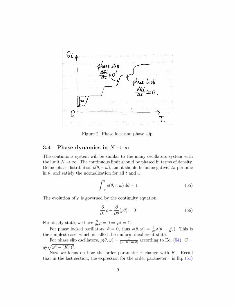
Figure 2: Phase lock and phase slip.

3.4 Phase dynamics in N → ∞The continuous system will be similar to the many oscillators system withthe limit N → ∞. The continuous limit should be phased in terms of density.Define phase distribution ρ(θ, τ, ω), and it should be nonnegative, 2π-periodicin θ, and satisfy the normalization for all t and ω:∫ π

−π

ρ(θ, τ, ω) dθ = 1 (55)

The evolution of ρ is governed by the continuity equation:

∂

∂τρ+

∂

∂θ(ρθ) = 0 (56)

For steady state, we have ∂∂τρ = 0 ⇒ ρθ = C.

For phase locked oscillators, θ = 0, thus ρ(θ, ω) = 12πδ(θ − ω

Kr). This is

the simplest case, which is called the uniform incoherent state.For phase slip oscillators, ρ(θ, ω) = C

|ω−Kr sin θ| according to Eq. (54). C =12π

√ω2 − (Kr)2.

Now we focus on how the order parameter r change with K. Recallthat in the last section, the expression for the order parameter r is Eq. (51)

9

r = 1N

∑Nj=1 e

iθj (Recall that Ψ = 0 by assumption). In the N → ∞ limit,the expression now becomes:

r =

∫ π

−π

∫ ∞

−∞eiθρ(θ, ω)g(ω) dθ dω (57)

where g(ω) is the frequency distribution normalized by∫∞−∞ g(ω) dω = 1

Using angular brackets to denote population averages, we have

⟨eiθ⟩ = ⟨eiθ⟩lock + ⟨eiθ⟩slip (58)

Note that ⟨eiθ⟩ = reiΨ = r. Thus

r = ⟨eiθ⟩lock + ⟨eiθ⟩slip (59)

Phase locked case: because g(ω) = g(−ω) and sin θi =ωi

Krfor the phase

locked case, we have ⟨sin θ⟩lock = 0. So

⟨eiθ⟩lock = ⟨cos θ⟩lock (60)

=

∫ Kr

−Kr

cos θ(ω)g(ω) dω (61)

= Kr

∫ π/2

−π/2

cos2 θg(Kr sin θ) dθ (62)

where θ(ω) is defined by sin θi =ωi

Kr.

Phase slip case:

⟨eiθ⟩slip =∫ π

−π

∫|ω|>Kr

eiθρ(θ, ω)g(ω) dθ dω (63)

because of the symmetry ρ(θ+π,−ω) = ρ(θ, ω) and g(ω) = g(−ω), the aboveintegral vanishes.

So in summary, we obtain the expression for the order parameter r:

r = Kr

∫ π/2

−π/2

cos2 θg(Kr sin θ) dθ (64)

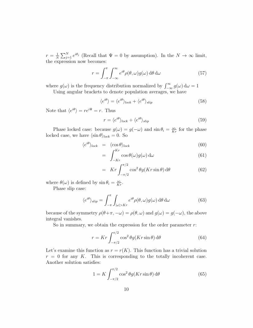
Let’s examine this function as r = r(K). This function has a trivial solutionr = 0 for any K. This is corresponding to the totally incoherent case.Another solution satisfies:

1 = K

∫ π/2

−π/2

cos2 θg(Kr sin θ) dθ (65)

10

This branch bifurcates continuously from r = 0 at a value K = Kc obtainedby letting r → 0+ in the above equation. Thus

Kc = 2/πg(0) (66)

where g(0) is a given function at a given value so it is known. This isKuramotos exact formula for the critical coupling at the onset of collectivesynchronization.

For r < 1, we can do the Taylor expansion:

g(Kr) = g(0) + g′(0)Kr sin θ +1

2g′′(0)(Kr sin θ)2 + ... (67)

Substituting it yields:

r ≃

√16

πK3c

õ

−g′′(0)(68)

where µ = K−Kc

Kc.

Near the onset, we have the scaling law:

∂r

∂K∼ 1√

K −Kc

(69)

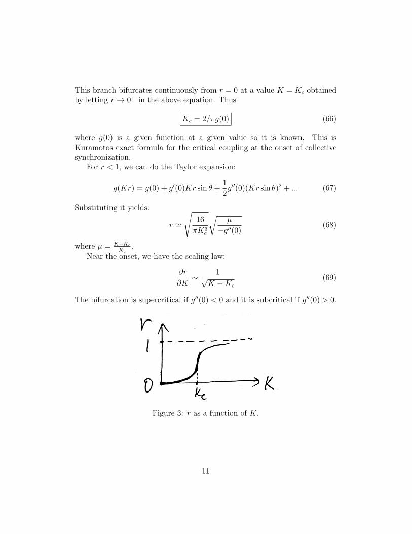
The bifurcation is supercritical if g′′(0) < 0 and it is subcritical if g′′(0) > 0.

Figure 3: r as a function of K.

11

References

[1] Yoshiki Kuramoto. Chemical oscillations, waves, and turbulence, vol-ume 19. Springer Science & Business Media, 2012.

[2] Arkady Pikovsky, Michael Rosenblum, and Jurgen Kurths. Synchroniza-tion: a universal concept in nonlinear sciences, volume 12. Cambridgeuniversity press, 2003.

[3] Steven H Strogatz. From kuramoto to crawford: exploring the onset ofsynchronization in populations of coupled oscillators. Physica D: Nonlin-ear Phenomena, 143(1):1–20, 2000.

12