Petra E. Todd Fall, 2016 - University of...

Lecture Notes 721: Discrete Choice Modeling

Petra E. Todd

Fall, 2016

Contents

i

ii CONTENTS

Chapter 1

Discrete choice modeling

Consider the classical regression model:

y = xβ + ε

E(ε|x) = 0

ε˜N(0, σ2)

This model is untenable if y is discrete. To model discrete choices, we needto think of the ingredients that give rise to choices.

For example, suppose we want to forecast the demand for a new good and weobserve consumption data on old goods, x1...xI . Each good might representa transportation mode or a type of car.

Assume that people choose the good that yields the highest utility. Whenwe have a new good, we need a way of putting it on a basis with the old.

1

2 CHAPTER 1. DISCRETE CHOICE MODELING

The earliest literature on discrete choice was developed in psychometricswhere researchers were concerned with modeling choice behavior.

There are two predominant modeling approaches:

(1) Luce (1953) Model ⇐⇒McFadden conditional logit model(2) Thurstone (1929) ⇐⇒Quandt multivariate probit/normal model

The Luce-McFadden model

• widely used in economics

• easy to compute

• identifiability of parameters well understood

• very restrictive substitution possibilities among goods

The Thurstone-Quandt model

• very general substitution possibilities

• allows for more general forms of heterogeneity

• more difficult to compute

• identifiability less easily established

1.1 Luce Model/McFadden conditional logit

model

Some references: Manski and Mcfadden; Greene; Amemiya

Notation:

X : universe of objects of choice

S : universe of attributes of people

B : feasible choice set

1.1. LUCE MODEL/MCFADDEN CONDITIONAL LOGIT MODEL 3

Behavior rule mapping attributes into choices:

h(B, s) = x

We might assume that there is a distribution of choice rules because

• in observation we lose some information governing choices

• there can be random variation in choices due to unmeasured psycho-logical factors

DefineP (x|s, B) = Pr(h ∈ H such that h(s, B) = x)

This represents the probability that an individual drawn randomly from thepopulation with attributes s and alternative set B chooses x.

Luce Axioms:

Maintain some restrictions on P (x|s, B) and derive implications for the func-tional form of P.

Axiom #1: Independence of Irrelevant Alternatives (IIA)

x, y ∈ B, s ∈ S

P (x|s, xy)P (y|s, xy)

=P (x|s, B)

P (y|s, B)

where B is a larger choice set

This means that other choices are irrelevant for the relative probabilityratio. This is not necessarily a reasonable assumption. For example, supposethe choice is a career decision and the possible choices are economist (E),policeman (P) and fireman (F). IIA implies

P (E|s, EF)P (F |s, EF)

=P (E|s, EFP)P (F |s, EFP)


This example is due to Stern. Does this restriction seem reasonable?

The restriction imposed on the substitution patterns is also known as theRed Bus-Blue Bus problem, which was first discussed by Debreu. Supposethe possible choices are modes of transportion car (c), red bus (RB), bluebus (BB). IIA implies:

P (c|s, c, RB)P (RB|s, c, RB)

=P (c|s, c, RB,BB)P (RB|s, c, RB,BB)

Axiom 2: Eliminate 0 probability choices

Pr(y|s, B) > 0 for all y ∈ B

Let’s analyze the implications of the above axioms:

Define Pxx = P (x|x, xx) and assume Pxx = 1/2

By IIA

P (y|s, B) =PyxPxy

P (x|s, B)

∑y∈B

P (y|s, B) = 1 =⇒ P (x|s, B) =1∑

y∈BPyxPxy

Furthermore, we have from IIA

P (y|s, B) =PyzPzy

P (z|s, B)

P (x|s, B) =PxzPzx

P (z|s, B)

P (y|s, B) =PyxPxy

P (x|s, B)

which implies

PyxPxy

=P (y|s, B)

P (x|s, B)=

PyzPzyPxzPzx

1.1. LUCE MODEL/MCFADDEN CONDITIONAL LOGIT MODEL 5

Define V (s, x, z) = ln(PxzPzx

) and V (s, y, z) = ln(PyzPzy

). Then we can write

PyxPxy

=eV (s,y,z)

eV (s,x,z)

Axiom 3: Separability assumption

Assume that V (s, x, z) = v(s, x)− v(s, z).V can be interpreted as a utility indicator of relative tastes

Then,

P (x|s, B) =1∑

y∈BPyxPxy

=1∑

y∈Bev(s,y)−v(s,z)

ev(s,x)−v(s,z)

=ev(s,x)∑y∈B e

v(s,y)

Thus, you can derive the multivariate logistic specification from the threeLuce Axioms.


1.2 Random Utility Models

Now, link to more familiar models in economics. Marshak (1959) estab-lished the link between the Luce model and so-called random utility models(RUMs). These kinds of models were proposed by Thurstone (1927, 1930’s)

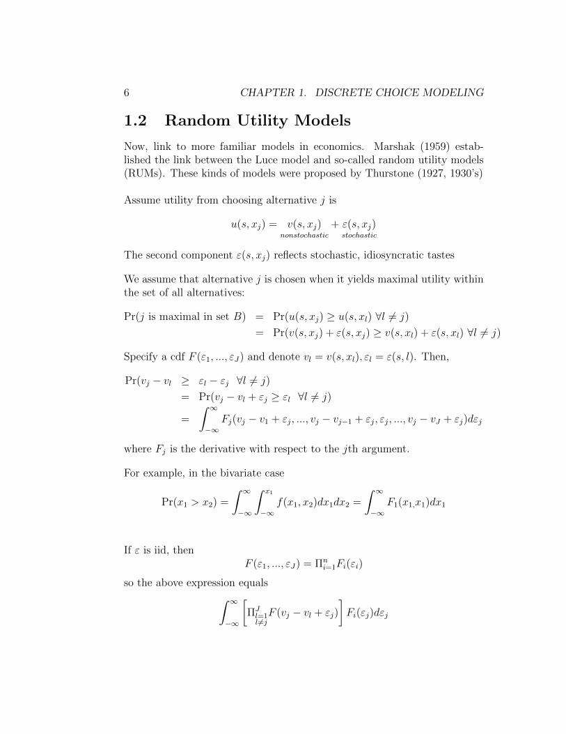
Assume utility from choosing alternative j is

u(s, xj) = v(s, xj)nonstochastic

+ ε(s, xj)stochastic

The second component ε(s, xj) reflects stochastic, idiosyncratic tastes

We assume that alternative j is chosen when it yields maximal utility withinthe set of all alternatives:

Pr(j is maximal in set B) = Pr(u(s, xj) ≥ u(s, xl) ∀l 6= j)

= Pr(v(s, xj) + ε(s, xj) ≥ v(s, xl) + ε(s, xl) ∀l 6= j)

Specify a cdf F (ε1, ..., εJ) and denote vl = v(s, xl), εl = ε(s, l). Then,

Pr(vj − vl ≥ εl − εj ∀l 6= j)

= Pr(vj − vl + εj ≥ εl ∀l 6= j)

=

∫ ∞−∞

Fj(vj − v1 + εj, ..., vj − vj−1 + εj, εj, ..., vj − vJ + εj)dεj

where Fj is the derivative with respect to the jth argument.

For example, in the bivariate case

Pr(x1 > x2) =

∫ ∞−∞

∫ x1

−∞f(x1, x2)dx1dx2 =

∫ ∞−∞

F1(x1,x1)dx1

If ε is iid, thenF (ε1, ..., εJ) = Πn

i=1Fi(εi)

so the above expression equals∫ ∞−∞

[ΠJl=1l 6=jF (vj − vl + εj)

]Fi(εj)dεj

1.2. RANDOM UTILITY MODELS 7

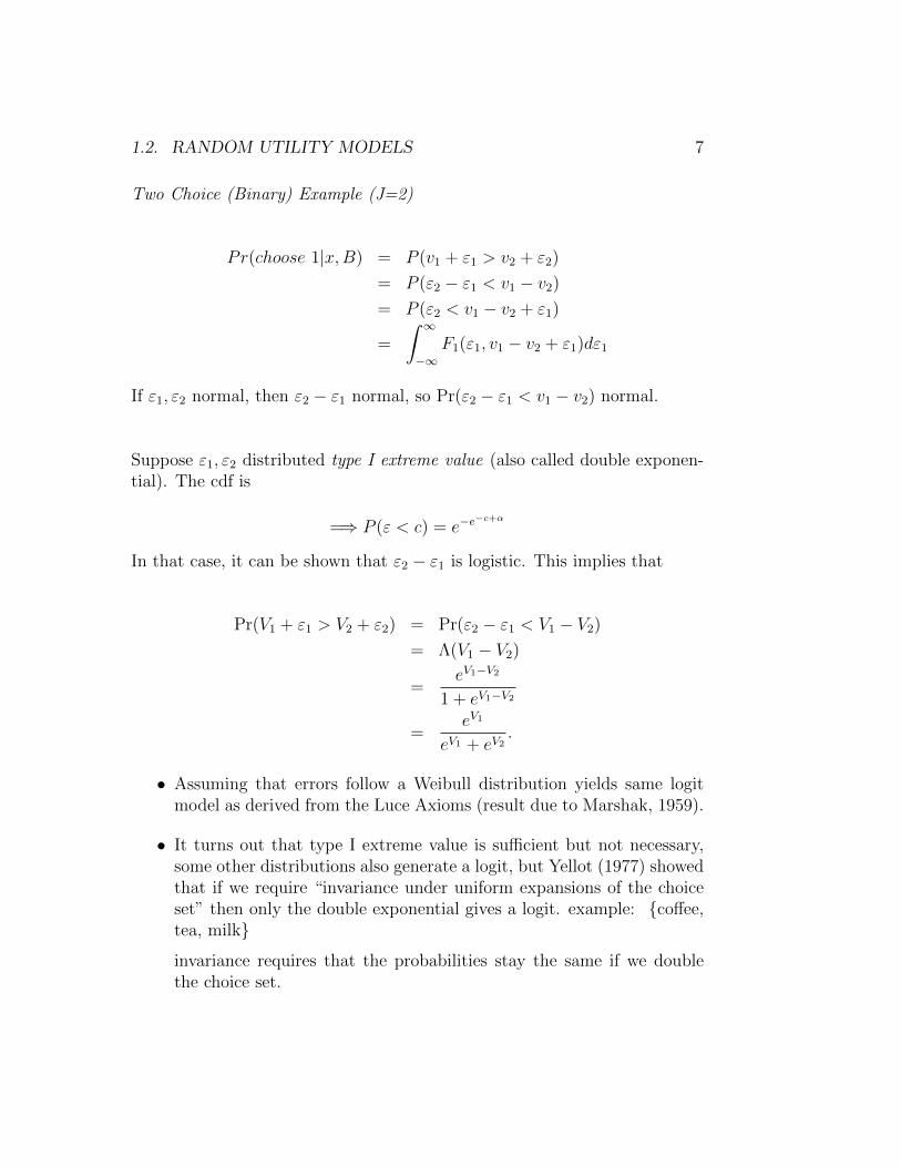
Two Choice (Binary) Example (J=2)

Pr(choose 1|x,B) = P (v1 + ε1 > v2 + ε2)

= P (ε2 − ε1 < v1 − v2)

= P (ε2 < v1 − v2 + ε1)

=

∫ ∞−∞

F1(ε1, v1 − v2 + ε1)dε1

If ε1, ε2 normal, then ε2 − ε1 normal, so Pr(ε2 − ε1 < v1 − v2) normal.

Suppose ε1, ε2 distributed type I extreme value (also called double exponen-tial). The cdf is

=⇒ P (ε < c) = e−e−c+α

In that case, it can be shown that ε2 − ε1 is logistic. This implies that

Pr(V1 + ε1 > V2 + ε2) = Pr(ε2 − ε1 < V1 − V2)

= Λ(V1 − V2)

=eV1−V2

1 + eV1−V2

=eV1

eV1 + eV2.

• Assuming that errors follow a Weibull distribution yields same logitmodel as derived from the Luce Axioms (result due to Marshak, 1959).

• It turns out that type I extreme value is sufficient but not necessary,some other distributions also generate a logit, but Yellot (1977) showedthat if we require “invariance under uniform expansions of the choiceset” then only the double exponential gives a logit. example: coffee,tea, milk

invariance requires that the probabilities stay the same if we doublethe choice set.


1.3 Solving the forecasting problem

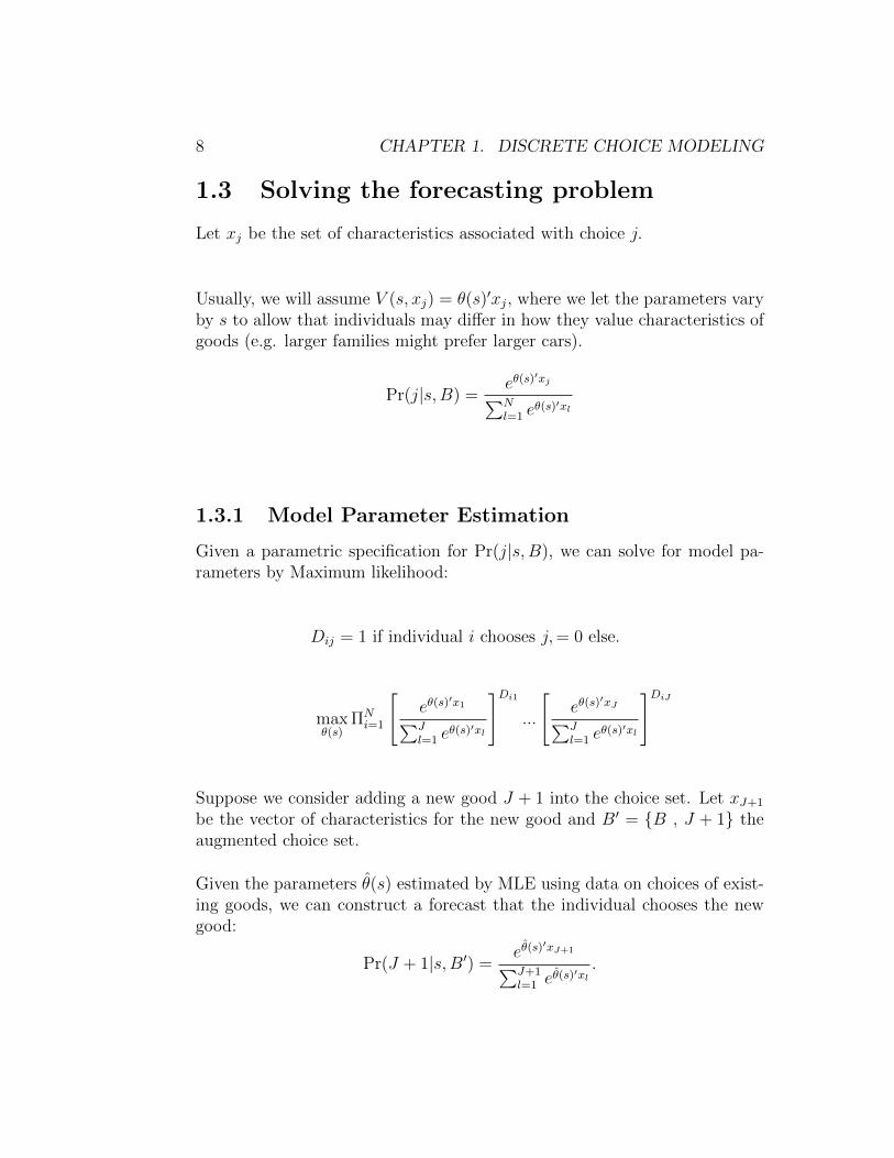
Let xj be the set of characteristics associated with choice j.

Usually, we will assume V (s, xj) = θ(s)′xj, where we let the parameters varyby s to allow that individuals may differ in how they value characteristics ofgoods (e.g. larger families might prefer larger cars).

Pr(j|s, B) =eθ(s)

′xj∑Nl=1 e

θ(s)′xl

1.3.1 Model Parameter Estimation

Given a parametric specification for Pr(j|s, B), we can solve for model pa-rameters by Maximum likelihood:

Dij = 1 if individual i chooses j,= 0 else.

maxθ(s)

ΠNi=1

[eθ(s)

′x1∑Jl=1 e

θ(s)′xl

]Di1...

[eθ(s)

′xJ∑Jl=1 e

θ(s)′xl

]DiJ

Suppose we consider adding a new good J + 1 into the choice set. Let xJ+1

be the vector of characteristics for the new good and B′ = B , J + 1 theaugmented choice set.

Given the parameters θ(s) estimated by MLE using data on choices of exist-ing goods, we can construct a forecast that the individual chooses the newgood:

Pr(J + 1|s, B′) =eθ(s)

′xJ+1∑J+1l=1 e

θ(s)′xl.

1.4. VERIFYING THAT A PROBABILITY CHOICE SYSTEM (PCS) IS CONSISTENTWITH A RANDOMUTILITYMODEL (RUM)9

1.3.2 Debreu criticism of Luce’s model

Suppose the J+1th alternative is identical to the first alternative. Then

Pr(choose 1 or J + 1|s, B′) =2eθ(s)

′xN+1∑J+1l=1 e

θ(s)′xl

• This means that introducing an identical good into the choice setchanges the probability of making that choice, which is not a desir-able result.

• The result comes from making an iid assumption on the error termassociated with the new alternative

U1 + ε1

UJ+1 + εJ+1

• If the goods are identical, then we would expect the error terms to beperfectly correlated, not iid. The iid assumption is at odds with thenotion of introducing a close (or identical) alternative.

1.4 Verifying that a probability choice sys-

tem (PCS) is consistent with a random

utility model (RUM)

What are criteria for a good probabilistic choice system?

1. has flexible functional form

2. is computationally practical

3. allows for flexibility in representing substitution patterns among choices

4. is consistent with a RUM (has a structural interpretation)


How do you verify whether consistent with a RUM?

• as shown earlier, we can start with a RUM and derive the PCS

Ui = V (s, xi) + ε(s, xi)

and solve integral for

Pr(U i > U l for all l 6= i) = Pr(V i + εi > V l + εl for all l 6= i)

• In some cases, we can start with PCS and verify that it is consistentwith a RUM using sufficient conditions

1.4.1 Daly-Zachary-Williams Theorem

Daly-Zachary (1976), Williams (1977)

Provides a set of conditions that make it easy to derive a PCS from a RUMwithin a class of models called generalized extreme value (GEV) models.

Define G = G(Y1, ..., YJ)

If G satisfies the following conditions:

1. nonnegative defined on Y1, ..., YJ ≥ 0

2. homogeneous of degree one in its arguments

3. limYi→∞G(Y1, ., Yi, ...YJ)→∞, for all i = 1..J

4. ∂kG∂Y1,...,∂Yk

is nonnegative if k is odd, and nonpositive if k is even

Then, for a RUM with Ui = Vi+εi and F (ε1, ..., εJ) = exp−G(e−ε1 , ..., e−εJ )the PCS is given by (with Yi = eVi)

Pi =∂ lnG

∂ lnYi=eViGi(e

V1 , ..., eVJ )

G(eV1 , ..., eVJ )

Remark: McFadden shows that under certain conditions on the form of Vi(satisfies AIRUM form), the DZW theorem can be seen as a form of Roy’sidentity.

Let’s apply the result:


(a) Multinomial logit model

F (ε1, ..., εJ) = e−e−ε1 ...e−e

−εJ

= e−∑Jj=1 e

−εj

Here,

G(eV1 , ..., eVJ ) =J∑j=1

eVj satisfies DZW conditions

Applying DZW, get the multinomial logit model (MNL) model:

Pi =∂ lnG

∂Vi=

eVi∑Jj=1 e

Vj

(b) Nested logit model (this model addresses to a limited extent the IIAcriticism)

G(eV1 , ..., eVJ ) =M∑m=1

am

[∑i∈Bm

eVi

1−σm

]1−σm

Idea is to first divide goods into M branches. First choose a branch andthen choose a good within a branch. Will allow for correlation betweenthe errors within a given branch.

Define Bm as a subset of the choice set:

Bm ⊆ 1, ..., Jm∪Mm=1Bm = B

Calculate the equation for Pi using the DZW result:

Pi =∂ lnGi

∂Vi=

∑m s.t. i∈Bm am

(e

Vi1−σm

) [∑i∈Bm e

Vi1−σm

]−σm∑M

m=1 am

[∑i∈Bm e

Vi1−σm

]1−σm

If we multiply by [∑i∈Bm

eVi

1−σm

]−1 [∑i∈Bm

eVi

1−σm

],


get

=M∑m=1

Pr(i|Bm) Pr(Bm),

where

Pr(i|Bm) =

(e

Vi1−σm

)∑

i∈Bm eVi

1−σm

if i ∈ Bm,= 0 otherwise

Pr(Bm) =am

[∑i∈Bm e

Vi1−σm

]1−σm

∑Mm=1 am

[∑i∈Bm e

Vi1−σm

]1−σm

How does the nested logit model accommodate the Red bus/Blue busproblem?

Suppose we have a nested set-up in which one branch contains onlychoice 1 and the other branch contains choice 2 and 3.

1

2 3


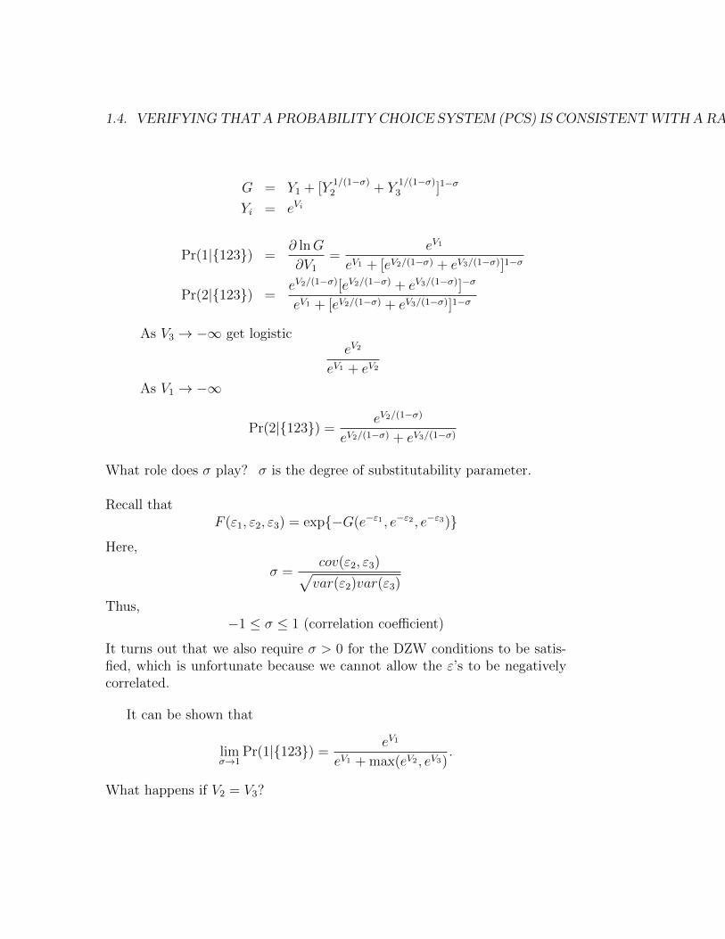
G = Y1 + [Y1/(1−σ)

2 + Y1/(1−σ)

3 ]1−σ

Yi = eVi

Pr(1|123) =∂ lnG

∂V1

=eV1

eV1 + [eV2/(1−σ) + eV3/(1−σ)]1−σ

Pr(2|123) =eV2/(1−σ)[eV2/(1−σ) + eV3/(1−σ)]−σ

eV1 + [eV2/(1−σ) + eV3/(1−σ)]1−σ

As V3 → −∞ get logisticeV2

eV1 + eV2

As V1 → −∞

Pr(2|123) =eV2/(1−σ)

eV2/(1−σ) + eV3/(1−σ)

What role does σ play? σ is the degree of substitutability parameter.

Recall thatF (ε1, ε2, ε3) = exp−G(e−ε1 , e−ε2 , e−ε3)

Here,

σ =cov(ε2, ε3)√var(ε2)var(ε3)

Thus,−1 ≤ σ ≤ 1 (correlation coefficient)

It turns out that we also require σ > 0 for the DZW conditions to be satis-fied, which is unfortunate because we cannot allow the ε’s to be negativelycorrelated.

It can be shown that

limσ→1

Pr(1|123) =eV1

eV1 + max(eV2 , eV3).

What happens if V2 = V3?


Then,

Pr(2|123) =eV2/(1−σ)[2eV2/(1−σ)]−σ

eV1 + [2eV2/(1−σ)]1−σ

=2−σeV2

eV1 + 21−σeV2

limσ→1

=1

2

eV2

eV1 + eV2,

This means you introduce an identical alternative and cut the probability ofchoosing good 2 by one half. This solves the Red-Bus-Blue-Bus problem.

Remark:

Can expand the nested logit to accommodate multiple levels. For exam-ple, three levels:

G =

Q∑q=1

aq

∑m∈Qq

am

[∑i∈Bm

Y1/(1−σm)i

]1−σm

1.4.2 Application: Choice of transportation mode

Let’s see how the model can be applied to the choice of transportion mode.This example is taken from Amemiya.

Suppose we assume that first a person chooses a neighborhood where tolive and then they choose a mode of transportation, given the set of choicesavailable within their neighborhood.

Neighborhood m

Transportation mode t

P (m) : probability of residing in neighborhood m

P (i|Bm) : probability of choosing ith mode, given live in neighborhood m

Not all modes may be available in each neighborhood. Let Tm denote the


number of modes available in neighborhood m.

Pm,t =ev(m,t)1−σm

[∑Tmt=1 e

v(m,t)1−σm

]−σm∑m

j=1

[∑Tjt=1 e

v(j,t)1−σm

]−σmPt|m =

ev(m,t)1−σm∑Tm

t=1 ev(m,t)1−σm

Pm =

[∑Tmt=1 e

v(m,t)1−σm

]1−σm

∑mj=1

[∑Tjt=1 e

v(j,t)1−σm

]1−σm

Standard type of utility function that people might use:

zt : trans. mode characteristics

xi : person characteristics

ym : neighborhood characteristics

V (m, t) = z′tγ + x′iβmt + y′mα

Could also include interaction terms between x and z and y.

Estimate by MLEΠMm=1Πn

i=1PDtmtm

where Dtm = 1 if person chooses mode t and neighborhood m, else Dtm = 0.

Chapter 2

Multinomial Probit Model

Main reference:

Bunch (1979) ”Estimability in the Multinomial Probit Model” in Transporta-tion Research

Applications of this model in Albreit, Lerman and Manski (1978), Hausmanand Wise (1978). Also, see Amemiya.

2.1 MNP Model

Consider a random utility model where j denotes the alternative,

Uj = Zjβ + ηj

= Zjβ + Zj(β − β) + ηjThis is an example of a random coefficients model, because the parameter β(which captures how people vary characteristics of the goods) is permittedto vary across people.

Assume there are J alternatives, K characteristics of the alternatives andthat β˜N(β,Σβ).

Define

ZJ×K βK×1 =

z′1β...

z′J β

η =

η1...ηJ

17

18 CHAPTER 2. MULTINOMIAL PROBIT MODEL

We will assume that η˜N(0,Ση).Then,

Pr(alternative j selected)=Pr(Uj > Ui for all i 6= j)

=

∫ ∞Uj=−∞

∫ Uj

U1=−∞...

∫ Uj

UJ=−∞φ(U |Vµ,Σµ)dUJ ...dU1dUj

Remarks:

• Here, φ is a J-dimensional multivariate normal density with mean Vµand variance Σµ.

• Unlike the MVL, no closed form expression exists for the integral inthe normal case. The integrals are therefore usually evaluated usingsimulation methods (as will be discussed later).

How many parameters are there?

β : K parameters

Σβ : K ×K symmetric matrix,K2 −K

2+K =

K(K + 1)

2parameters

Ση :J(J + 1)

2parameters

When a person chooses alternative j, all we know is relative utility, notabsolute utility. This suggests that not all the parameters in the model willbe identified. We will therefore require some normalizations.

2.2 Identification

What does it mean to say a parameter is identified in a model? If aparameter or set of parameters is not identified, then a model with one

2.2. IDENTIFICATION 19

parameterization is observationally equivalent to a model with a differentparameterization.

Example: Binary probit model (with fixed β)

Consider the case where a person is making a choice between 1 and 2. LetD denote the choice. Let Xi denote characteristics of the individual.

Pr(D = 1|Xi) = Pr(V1 + ε1 > V2 + ε2)

= Pr(Xiβ1 + ε1 > Xiβ2 + ε2)

= Pr(Xi(β1 − β2) > ε2 − ε1)

= Pr(Xi(β1 − β2)

σ>ε2 − ε1

σ)

= Φ(Xiβ

σ), where β = β1 − β2

Φ(Xiβσ

) is observationally equivalent to Φ(Xiβ∗

σ∗) for β

σ= β∗

σ∗, so β is not sepa-

rately identified relative to σ.

But the ratio is identified. Suppose

Φ(Xiβ

σ) = Φ(

Xiβ∗

σ∗)

Φ−1Φ(Xiβ

σ) = Φ−1Φ(

Xiβ∗

σ∗)

n∑i=1

X ′iXi(β

σ) =

n∑i=1

X ′iXi(β∗

σ∗)

which impliesβ

σ=

β∗

σ∗

The setb : b = βγ, γ any positive scalar is identified

Note that we assumed that∑n

i=1 X′iXi is invertible. We would say that “β

is identified up to scale and also that the sign is identified” (because σ mustbe positive).


Definition of Identification

For a parameter space B and a random vector Z, identification is selectinga subset in B that characterizes some aspect of the probability distributionof Z.

Now, return to identification in the MVP model.

Pr(j selected |Vµ,Σµ) = Pr(Ui − Uj < 0 for all i 6= j)

Define the contrast matrix

∆j =

1 0 . . . −1 . . . 0

−1 0

0...

...0 −1 0 1

(J−1)×J

∆jU =

U1 − U j

...UJ − U j

Pr(j selected |Vµ,Σµ) = Pr(∆jU < 0|Vµ,Σµ)

= Φ(0|VZ ,ΣZ)

where

VZ is the mean of ∆jU , which is ∆jZβ

ΣZ is the variance, which is ∆jZΣβZ′∆′j + ∆jΣη∆

′j

VZ is (J − 1)× 1

ΣZ is (J − 1)× (J − 1)

Here, we reduced the dimension of the integration problem by one. This rep-resentation shows that all the information is in the contrasts and we thereforecannot identify all of the components of Vµ and Σµ.

2.2. IDENTIFICATION 21

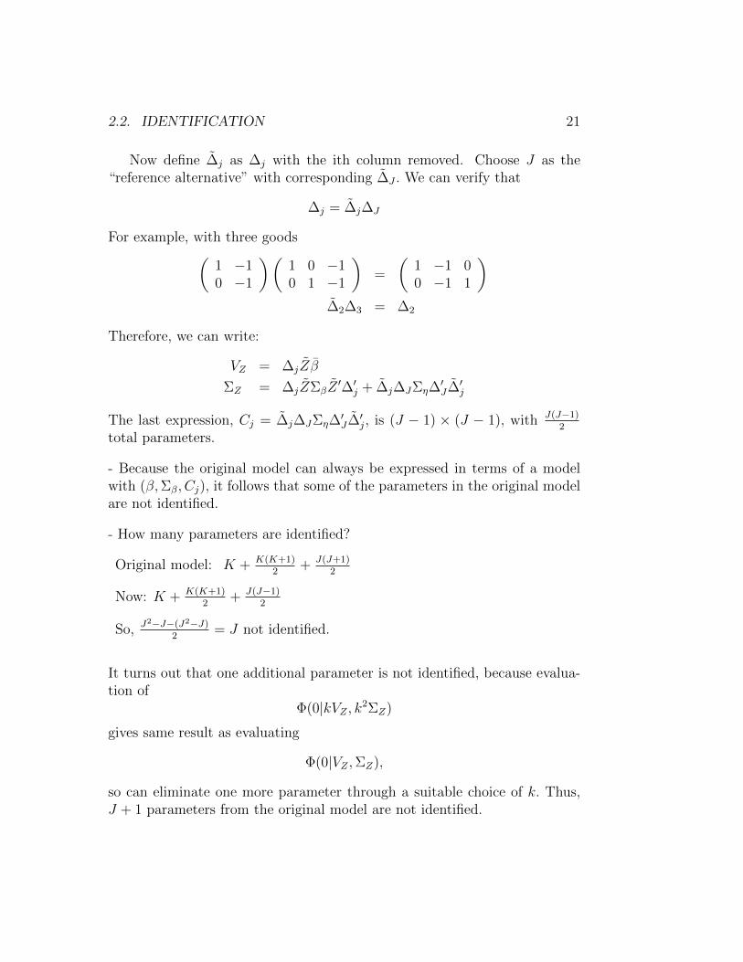
Now define ∆j as ∆j with the ith column removed. Choose J as the“reference alternative” with corresponding ∆J . We can verify that

∆j = ∆j∆J

For example, with three goods(1 −10 −1

)(1 0 −10 1 −1

)=

(1 −1 00 −1 1

)∆2∆3 = ∆2

Therefore, we can write:

VZ = ∆jZβ

ΣZ = ∆jZΣβZ′∆′j + ∆j∆JΣη∆

′J∆′j

The last expression, Cj = ∆j∆JΣη∆′J∆′j, is (J − 1) × (J − 1), with J(J−1)

2

total parameters.

- Because the original model can always be expressed in terms of a modelwith (β,Σβ, Cj), it follows that some of the parameters in the original modelare not identified.

- How many parameters are identified?

Original model: K + K(K+1)2

+ J(J+1)2

Now: K + K(K+1)2

+ J(J−1)2

So, J2−J−(J2−J)2

= J not identified.

It turns out that one additional parameter is not identified, because evalua-tion of

Φ(0|kVZ , k2ΣZ)

gives same result as evaluating

Φ(0|VZ ,ΣZ),

so can eliminate one more parameter through a suitable choice of k. Thus,J + 1 parameters from the original model are not identified.


Illustration of how to impose normalization

J = 3

Ση =

σ11 σ12 σ13

σ21 σ22 σ23

σ31 σ32 σ33

Set 3 as the reference alternative:

C3 = ∆3Ση∆′3

=

(1 0 −10 1 −1

)Ση

(1 0 −10 1 −1

)′=

(σ11 − 2σ31 + σ33 σ21 − σ31 − σ32 + σ33

σ21 − σ31 − σ32 + σ33 σ22 − 2σ32 + σ33

)

Only combinations of parameters are identified. For example,

∆2∆3Ση∆′3∆′2

=

(1 −10 −1

)(σ11 − 2σ31 + σ33 σ21 − σ31 − σ32 + σ33

σ21 − σ31 − σ32 + σ33 σ22 − 2σ32 + σ33

)(1 0−1 −1

)

Normalization approach of Albreit, Lerman and Manski (1978):

- need J + 1 restrictions on the VCV matrix

- fix J parameters by settings last row and last column of Ση to 0

- fix the scale by constraining the diagonal elements of Ση so that trace(ΣεJ

)equals the variance of a standard log Weibull (they compare estimatesof MNL with those of a MNP and of an independent MNP).

2.3. HOW DO WE SOLVE THE FORECASTING PROBLEM? 23

2.3 How do we solve the forecasting prob-

lem?

Suppose we have two goods and add a third.

Pr(choose 1|Z1, Z2) = Pr(U1 − U2 ≥ 0)

= Pr((Z1 − Z2)β ≥ w2 − w1)

where

w1 = Z1(β − β) + η1

w2 = Z2(β − β) + η2

Because w2 − w1 is normally distributed,∫ (Z1−Z2)β

[σ11+σ22−2σ12+(Z2−Z1)Σβ(Z2−Z1)′]1/2

−∞

1√2πe−t/2dt

Now add a third good:

U3 = Z3β + Z3(β − β) + η3

Problem is that we don’t know the correlation of η3 with the other errors.

Suppose we knew that η3 = 0 (i.e. only preference heterogeneity)

Then

Pr(1 is chosen)=

∫ a

−∞

∫ b

−∞BV Ndt1dt2

where BVN = bivariate normal density and

a =(Z1 − Z2)β

[σ11 + σ22 − 2σ12 + (Z2 − Z1)Σβ(Z2 − Z1)′]1/2

b =(Z1 − Z3)β

[σ11 + (Z2 − Z1)Σβ(Z3 − Z1)′]1/2

We could also solve the forecasting problem if we make an assumptionlike η2 = η3.


2.4 Application from Hausman and Wise (1978)

Develop a model of commuting choices for workers in Washington, D. C.

Choice of

(a) driving car

(b) sharing ride

(c) riding bus

Utility model for person i choosing mode j

Uij = βi1 log x1ij + βi2 log x2ij + βi3x3ij

x4i

+ εij

x1ij = time in vehicle

x2ij = time out of vehicle

x3ij = cost of mode for that person

x4i = income of person

Chapter 3

Simulation Methods for MNPmodels

MNP models tend to be difficult to estimate because of high dimensionalintegrals that need to be evaluated at each stage of evaluating the likelihood.

There are a variety of simulation methods that have been developed forestimating these types of models. Two popular methods are:

• Simulated method of moments (SMOM)

• Simulated maximum likelihood (SMLE)

References :

Lerman and Manski (1981) - Structual Analysis of Discrete Data

McFadden (1989) Econometrica

Ruud (1982) Journal of Econometrics

Hajivassilou and Ruud, Ch. 20, Handbook of Econometrics, Stern (1992)Econometrica

Stern (1997) survey article in Journal of Economic Literature

Gourieroux, Christin and Alain Monfort (2002): Simulation-Based Econo-metric Methods

25

26 CHAPTER 3. SIMULATION METHODS FOR MNP MODELS

Geweke, John and Michael Keane (2001): “Computationally intensive meth-ods for integration in econometrics,” Handbook of Econometrics, Vol.5.

3.1 Early simulation method - crude frequency

method

Consider a model with only taste heterogeneity but no preference hetero-geneity:

Uj = Zjβ + ηj

β fixed

ηj˜N(0,Ω)

J choices

Let

Pij = prob person i chooses j

Yij = 1 if i chooses j,= 0 else

The likelihood can be written as

L = ΠNi=1ΠJ

j=1(Pij)Yij

logL =N∑i=1

J∑j=1

Yij logPij

=N∑i=1

logPik

where N denotes the number of individuals and k is the alternative chosenby individual i.

3.1. EARLY SIMULATIONMETHOD - CRUDE FREQUENCYMETHOD27

Simulation Algorithm:

1. For a given β,Ω generate R Monte Carlo draws of the vector of resid-uals, η

2. Let

Pk =1

R

R∑r=1

1(U rk = maxU r

1 , ..., UrJ)

Pk is a frequency simulator of the proportion of times that k is chosengiven β,Ω

3. Maximize∑N

i=1 log Pik over alternative values for β,Ω.

Lerman and Manski found that this procedure performs poorly and requiresa large number of draws to be accurate, particularly when P is close to 0 or 1.

Variance of the frequency simulator is 1R2RV ar(1()) = Pk(1−Pk)

R.

McFadden (1989) provided some insights into how to improve the simulationmethod. He showed that simulation is a viable method of estimation evenfor a small number of draws provided that

(a) an unbiased simulator is used

(b) functions that are simulated appear linearly in the conditions definingthe estimator

(c) same set of random draws is used to simulate the model at differentparameter values

Condition (b) is violated for the crude frequency simulator, which has logPik.


3.2 Simulated method of moments

Consider model we had before, but with only preference heterogeneity andno taste heterogeneity:

Uij = Zijβ = Zijβ + Zijεi

β = β + εi

Define

Pij(γ) = Pr(i chooses j|Zi, β,Σε)

Yij = 1 if i chooses j,= 0 else

The likelihood is given by:

logL =1

N0

N∑i=1

J∑j=1

Yij lnPij(γ), N0 = NJ

∂ logL

∂γ=

1

N0

N∑i=1

J∑j=1

Yij

∂Pij∂γ

Pij(γ)

= 0 (*)

Now use the fact that

J∑j=1

Pij(γ) = 1

which impliesJ∑j=1

∂Pij∂γ

= 0

andJ∑j=1

∂Pij∂γ

PijPij = 0.

We can therefore rewrite (*) as

1

N0

N∑i=1

J∑j=1

(Yij − Pij)

∂Pij∂γ

Pij(γ)

= 0

3.2. SIMULATED METHOD OF MOMENTS 29

Note that E(Yij) = Pij. Letting Zij =∂Pij∂γ

Pij(γ)and εij = Yij − Pij, we have

1

N0

N∑i=1

J∑j=1

εijZij = 0,

which is like a moment condition using Zij as an instrument. So far, Pij isstill a J-1 dimensional integral.

The method of simulated moments solves the first-order conditions.

Model:

Uij = Zijβ + Zijεij

Ui = Ziβ + ZΓei

Ui is J × 1

Zi is J ×Kei is K × 1

Γ is K ×K

ΓΓ′ = Σε (cholesky decomposition)

ei˜N(0, Ik)

Simulation algorithm:

(i) Generate ei for each i such that ei are iid across persons and distributedN(0, Ik). In total, generate NKR draws, where N is the sample size, Kis the number of characteristics, and R is the number of Monte Carlodraws.

(ii) Fix matrix Γ and obtainηij = ZijΓei

and form vector zi1Γeizi2Γei

...ziJΓei

for each person.


(iii) Fix β and generate:Uij = Zijβ + ηij

for all i.

(iv) Find relative frequency that the ith person chooses alternative j acrossMonte Carlo draws:

Pij(γ) =1

R

R∑r=1

1(Ui1 > Uim for all m 6= j)

Pij(γ) is a simulator for Pij(γ). Stack to get Pi(γ).

(v) To get Pij(γ) for different values of γ, repeat steps (i) through (iv) usingthe same random variable draws ei from step (i).

(vi) Obtain a numerical simulator for∂Pij∂γ

: For small h,

∂Pij(γ)

∂γ=Pij(γ + hem)− Pij(γ − hem)

2h

where em is a vector with a 1 in the mth place.

Now, we have the ingredients for evaluating the moment conditions. Canuse a method such as Gauss-Newton method to solve the moment conditions.

Limitations of Simulation Methods

1. Pij(γ) simulator not smooth due to presence of indicator function (causesdifficulties in deriving the asymptotic distribution - need to use methodsdeveloped by Pakes and Pollard (1989) for nondifferentiable functions)

2. Pij cannot equal 0 (causes problems in denominator when close to 0)

3. Simulating a small Pij may require a large number of draws

Refinement: “Smoothed Simulated Method of Moments” by S. Stern (1992,Econometrica)

3.2. SIMULATED METHOD OF MOMENTS 31

Replaces the indicator function with a smooth function, which is differen-tiable

Pij(γ) =1

R

R∑r=1

k(Uij − Uim)

The smoothed function goes smoothly from 0 to one around 0 instead ofchanging abruptly at 0.

How does simulation affect the asymptotic distribution?

Define

Wi =

∂Pi∂γ

Pi(γ).

The variance of the method of moments estimator is given by

D(γ) = plim[1

N

N∑i=1

W ′i

∂Pi∂γ

]−1

plim[1

N

N∑i=1

(1 +1

R)Pi(1− PI)W ′

iWi]

plim[1

N

N∑i=1

W ′i

∂Pi∂γ

]−1

where the term 1R

adjusts for the simulation error.

Remarks:

• An advantage of simulated methods of moments over simulated maxi-mum likelihood methods is that SMM does not require that the numberof draws (R) goes to infinity and in fact has been shown to performwell even for a modest number of draws.

• Simulated maximum likelihood (where the simulator is plugged directlyinto the likelihood instead of working with the FOC, does require thatthe number of draws go to infinity.

Chapter 4

Nonrandom sampling

References: Amemiya (Chapter 9 and 10), Manski and McFadden (Chapters1 and 2), Manski and Lerman (1978 Econometrica), Amemiya

Different Types of Sampling

• random sampling

• censored sampling

• truncated sampling

• other nonrandom

– exogenous stratified sampling

– endogenous stratified (choice-based) sampling

- For example, in administering surveys, there is often oversampling ofhigh density population areas (often done to reduce sampling costs or to in-crease representation of certain groups). The sampling could be consideredto be exogenous or endogenous, depending on the phenomenon being studied.

- Most estimators are developed assuming random sampling and adjust-ments usually need to be made to accommodate nonrandom sampling situ-ations.

- Datasets usually provide sampling weights that are required to adjustfor the nonrandom sampling

33

34 CHAPTER 4. NONRANDOM SAMPLING

4.1 Some examples of choice-based sampling

• Suppose we want to study transportation mode choices and we gatherdata at the train, station, subway station, and at car checkpoints (e.g.toll booths).

• Study the effectiveness of a new treatment for heart attacks and followpeople who have had the treatment along with a control group of peo-ple who have not had the treatment.

• Evaluate the effects of a job training program using data on a group ofprogram participants and a group of nonparticipants. Participants areoften oversampled relative to their frequency in a random population.

In all of these cases, we observe characteristics of populations conditionalon the choices they made. Let’s look at how to use weights can be used toadjust for choice-based sampling:

Let Pi = P (i |Zi) in a random sample.

Let P ∗i the corresponding probability in a choice-based sample.

Under choice-based sampling, sampling is random within i partitions of thedata

P (Z |i) = P ∗(Z |i)

but

P (Z) 6= P ∗(Z).

Suppose we want to recover P (i |Z) from choice-based sampled data. Weobserve:

P ∗(i |Z)

P ∗(Z)

P ∗(i)

4.1. SOME EXAMPLES OF CHOICE-BASED SAMPLING 35

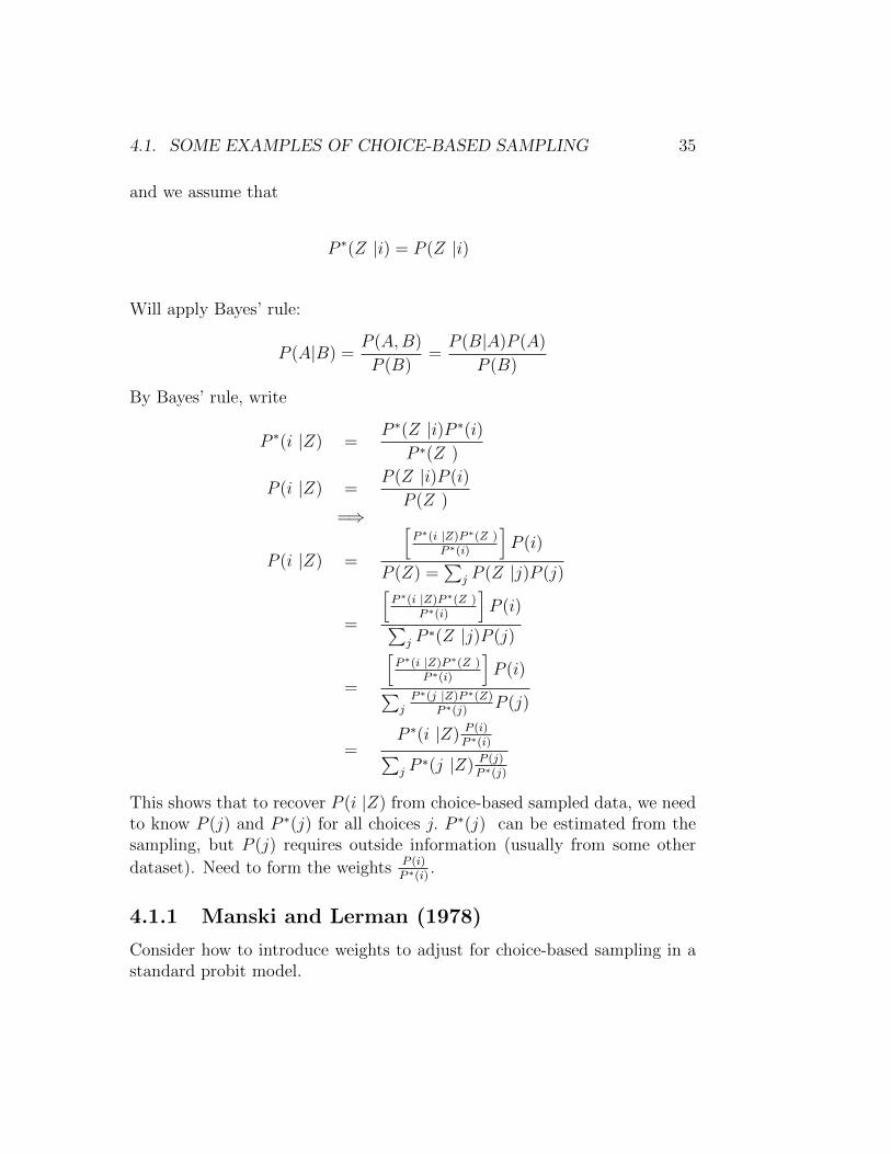
and we assume that

P ∗(Z |i) = P (Z |i)

Will apply Bayes’ rule:

P (A|B) =P (A,B)

P (B)=P (B|A)P (A)

P (B)

By Bayes’ rule, write

P ∗(i |Z) =P ∗(Z |i)P ∗(i)

P ∗(Z )

P (i |Z) =P (Z |i)P (i)

P (Z )=⇒

P (i |Z) =

[P ∗(i |Z)P ∗(Z )

P ∗(i)

]P (i)

P (Z) =∑

j P (Z |j)P (j)

=

[P ∗(i |Z)P ∗(Z )

P ∗(i)

]P (i)∑

j P∗(Z |j)P (j)

=

[P ∗(i |Z)P ∗(Z )

P ∗(i)

]P (i)∑

jP ∗(j |Z)P ∗(Z)

P ∗(j)P (j)

=P ∗(i |Z) P (i)

P ∗(i)∑j P∗(j |Z) P (j)

P ∗(j)

This shows that to recover P (i |Z) from choice-based sampled data, we needto know P (j) and P ∗(j) for all choices j. P ∗(j) can be estimated from thesampling, but P (j) requires outside information (usually from some other

dataset). Need to form the weights P (i)P ∗(i)

.

4.1.1 Manski and Lerman (1978)

Consider how to introduce weights to adjust for choice-based sampling in astandard probit model.

36 CHAPTER 4. NONRANDOM SAMPLING

Binary choice model

Di = 1 if xiβ + εi > 0

= 0 else

Denote choice-based sampling weights

w1i =P (Di = 1)

P ∗(Di = 1)

w0i =P (Di = 0)

P ∗(Di = 0)

Likelihood

L =1

NΠni=1 [1− Φ(−xiβ)]w1iDi [Φ(−xiβ)]w0i(1−Di)

In logs,

logL =1

N

n∑i=1

(w1iDi)log[1− Φ(−xiβ)] + (w0i(1−Di)log[Φ(−xiβ)]

As N gets large, DiN

converges to P ∗(Di = 1) and 1−DiN

to P ∗(Di = 0), sothat incorporating the weights, log L converges to E(logL).

Chapter 5

Limited Dependent VariableModels

main reference: Amemiya

In discrete choice models, we observe which choice is made from a set ofalternatives along with some observable covariates of the individual and/orof the choices.

We next consider a class of models where the outcome variables are partiallyobserved, called limited dependent variable models.

5.1 Type I Tobit Model

In Tobin’s (1958) example: expenditure on a durable good (e.g. a refrigera-tor) is only observed if the good is purchased. Some people chose not to buythe good, but might have bought it had the price been lower.

Define a latent variable that represents desired expenditure amount on agood:

y∗i = xiβ + ui

37

38 CHAPTER 5. LIMITED DEPENDENT VARIABLE MODELS

We observe

yi = y∗i if y∗i ≥ y0

= 0 if y∗i < y0

where y0 is the minimum price available in the market. Or, we can write

yi = 1(yi ≥ y0)y∗i .

Estimation

We can assume a parametric specification on the error term:

ui˜N(0, σ2)

y∗i |xi˜N(xiβ, σ2u)

Di = 1 if y∗i ≥ y0,

= 0 else

The likelihood can be written as

L = Πni=1 Pr(y∗i < y0) (1−Di) Pr(y∗i ≥ y0)f(y∗i |y∗i ≥ y0) Di .

Pr(y∗i < y0) = Pr(xiβ + uiσu

<y0

σu) = Φ

(y0 − xiβσu

)

f(y∗i |y∗i ≥ y0) =

1σuφ(y∗i−xiβσu

)1− Φ

(y0−xiβσu

)Now, note that the likelihood can be written as:

L = ΠDi=0

Φ

(y0 − xiβσu

)Π

Di=1

1− Φ

(y0 − xiβσu

)Π

Di=1


)1− Φ

(y0−xiβσu

)Remarks

(i) The first two products are the information that you would get fromwhether y∗i ≥ y0 (i.e. whether bought the good or not). This infor-mation alone could be used to estimate β up to scale by a binary probit.

(ii) With the additional information on expenditure (y∗i ), can get a more ef-ficient estimate of β/σu and an estimate of σu, which was not identifiedfrom only the information on whether the good was purchased.

5.1. TYPE I TOBIT MODEL 39

5.1.1 Truncated Type I Tobit Model

Suppose you only observe expenditure for the cases when the good was pur-chased. That is, you see y∗i for y∗i ≥ y0.

For example, maybe you gather your data at the appliance store interviewingpeople who purchase the good.

In that case, you have less information and the likelihood is:

L = ΠDi=1


)1− Φ

(y0−xiβσu

)It is still possible to estimate the model parameters using the truncated data.

5.1.2 Different Ways of Estimating Tobit Models

(a) MLE, or

(b) If Censored, can use a two step approach.

(c) Nonlinear least squares

Two Step Approach (due to Heckman, 1974, 1976)

First, estimate probit model using only data on whether good is purchased,get β

σu

Then estimate OLS model on observations for which y∗i is observed. Forexample, with y0 = 0 :

E(yi|xiβ + ui ≥ 0) = xiβ + E(ui|xiβ + ui ≥ 0)

= xiβ + σuE(uiσu| uiσu≥ −xiβ

σu)

for ε˜N(0, 1)


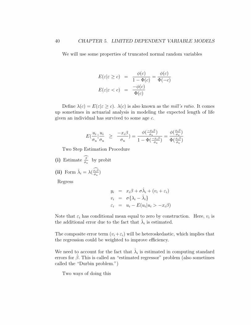
We will use some properties of truncated normal random variables

E(ε|ε ≥ c) =φ(c)

1− Φ(c)=

φ(c)

Φ(−c)

E(ε|ε < c) =−φ(c)

Φ(c)

Define λ(c) = E(ε|ε ≥ c). λ(c) is also known as the mill’s ratio. It comesup sometimes in actuarial analysis in modeling the expected length of lifegiven an individual has survived to some age c.

E(uiσu| uiσu≥ −xiβ

σu) =

φ(−xiβσu

)

1− Φ(−xiβσu

)=φ(xiβ

σu)

Φ(xiβσu

)

Two Step Estimation Procedure

(i) Estimate βσu

by probit

(ii) Form λi = λ( xiβσu

)

Regress

yi = xiβ + σλi + (vi + εi)

vi = σλi − λiεi = ui − E(ui|ui > −xiβ)

Note that εi has conditional mean equal to zero by construction. Here, vi isthe additional error due to the fact that λi is estimated.

The composite error term (vi+εi) will be heteroskedastic, which implies thatthe regression could be weighted to improve efficiency.

We need to account for the fact that λi is estimated in computing standarderrors for β. This is called an “estimated regressor” problem (also sometimescalled the “Durbin problem.”)

Two ways of doing this

5.2. TYPE II TOBIT MODEL 41

- Delta method

- GMM (Newey, Economic Letters, 1984) - set up moment conditions forthe OLS estimation and for the probit estimation program, with opti-mal weighting matrix. Estimating jointly will give corrected standarderrors.

(Correction for estimated regressor is incorporated into stata).

Nonlinear least squares approach

Suppose you used all the data, including the zeros,

E(yi|xi) = Pr(y∗i < 0) · 0 + Pr(y∗i > 0)E(y∗i |y∗i ≥ 0)

= Φ

(xiβ

σu

)[xiβ + σuλ(

xiβ

σu)

]

Could estimate by ols, replacing Φ with Φ and λ with λ, or could do nonlinearleast squares.

5.2 Type II Tobit Model

In the previous model, the outcome was observed based on whether the out-come exceeded a threshold value.

With Type II Tobit, we have one equation that describes the outcome andanother equation that describes when the outcome is observed, called theswitching equation:

y∗1i = x1iβ + u1i

y∗2i = x2iβ + u2i

y2i = y∗2i if y∗1i ≥ 0

= 0 else

Here, we observe x1i and x2i. y∗1i is not directly observed, although we observe

whether y∗1i ≥ 0. y2i is only observed if y∗1i ≥ 0.


5.2.1 The likelihood:

The likelihood for this Type II Tobit model is:

L = Π1

Pr(y∗1i ≥ 0)f(y2i|y∗1i ≥ 0)Π0

Pr(y∗1i < 0)

where

f(y2i|y∗1i ≥ 0) =

∫∞0f(y∗1i, y

∗2i)dy

∗1i∫∞

0f(y∗1i)dy

∗1i

= f(y∗2i)

∫∞0f(y∗1i|y∗2i)dy∗1i∫∞

0f(y∗1i)dy

∗1i

,

where f(y∗2i) and f(y∗1i) are the marginal densities.

Assume

y∗1iÑ(x1iβ1, σ21)

y∗2iÑ(x2iβ2, σ22)

We will use the following properties of conditional densities:

y∗1i|y∗2iÑ(x1iβ1 +σ12

σ22

(y∗2i − x2iβ2), σ21 −

σ12

σ22

)

y∗2i|y∗1iÑ(x2iβ2 +σ12

σ21

(y∗1i − x1iβ2), σ22 −

σ12

σ21

)

Estimation by MLE:

L = Π0

[1− Φ

(x1iβ1

σ1

)]Π1Φ

(x1iβ1

σ1

)f(y∗2i)

∫∞0f(y∗1i|y∗2i)dy∗1i∫∞

0f(y∗1i)dy

∗1i

= Π0

[1− Φ

(x1iβ1

σ1

)]×

Π1

φ(y2i−x2iβ2

σ2

)σ2

1− Φ

(−x1iβ1 + σ12

σ22

(y2i − x2iβ2)σ∗

)

σ∗ =

√σ2

1 −σ12

σ22


The likelihood depends on σ1 only through β1σ−11 and σ12/σ

−11 , so we

cannot separately identify σ1 and WLOG can impose a normalization suchas σ1 = 1.


Estimation by Two Step Approach

Using data on y2i for which y1i > 0.

E(y2i|y∗1i > 0) = x2iβ2 + E(u2i|x1iβ1 + u1i > 0)

= x2iβ2 + σ2E(u2i

σ2

|u1i

σ1

>−x1iβ1

σ1

)

= x2iβ2 +σ12

σ1

E(u1i

σ1

|u1i

σ1

>−x1iβ1

σ1

)

= x2iβ2 + αφ(−x1iβ1

σ1

)1− Φ(−x1iβ1

σ1)

= x2iβ2 + αλ

(−x1iβ1

σ1

)

5.2.2 Examples

Estimating the effect of school quality on school-going behaviorand on test scores in a developing country

Suppose we wish to assess how improving the quality of schools in a countrywould affect school-going behavior and test scores.

Quality might be measured in terms of school infrastructure (e.g. type ofroof, whether there is a bathroom), textbooks or teacher characteristics (ex-perience, degrees).

Suppose the tests are given in school and we only observe test scores forchildren who go to school. However, we observe for all children whether theygo to school.

y2i = student’s test scores

y1i = index representing parent’s propensity

to enroll child in school


x1i and x2i might both include school quality along with other covariates.For example, distance to school could be a favor influencing whether a familysends their child to school (i.e. included in x1i but not in x2i).

Gronau’s Female Labor Supply Model

maxC,L

U(C,L)

C = wH + A

H = 1− Lw = wage rate (given)

Pc = 1

L = time spent at home for child care

First-order condition:

MRS =∂U∂L∂U∂C

= w when L < 1

∂U∂L∂U∂C

> w if L = 1

Define reservation wagewR = MRS |H=0.

We don’t observe reservation wage directly, so model

wo = xβ + u wage offer

wR = zγ + v reservation wage.

Only observe the wage offer if the offer exceeds the reservation wage:

wi = woi if woi > wRi= 0 else.


This model fits within the Tobit Type II framework if we set

y∗1i = xiβ − ziγ + ui − vi = woi − wRiy∗2i = woi

Gronau did not develop a model to explain the choice of H (hours worked).

5.3 Type III Tobit: Heckman’s Model (In-

corporates Choice of H)

Adopts a functional form for the utility function that implies a functionalform relationship between the marginal rate of substitution and hours worked:

woi = x2iβ2 + u2i

MRS = γHi + ziα + vi

MRS |H=0 = wR = ziα + vi

An individual works if

woi > wRi , or

x2iβ2 + u2i > ziγ + vi

If works, then

woi = MRS

=⇒ x2iβ2 + u2i = γHi + ziα + vi

=⇒ Hi =x2iβ2 − ziα + u2i − vi

γ= x1iβ1 + u1i

where

x1iβ1 = (x2iβ2 − ziα)γ−1

u1i = (u2i − vi)γ−1

Observe both hours and wages (two outcomes) if hours worked is positive:

5.4. TYPE IV TOBIT MODEL 47

y∗1i = x1iβ1 + u1i hours (= Hi)

y∗2i = x2iβ2 + u2i wages (= w∗i )

y1i = y∗1i if y∗1i > 0

= 0 if y∗1i ≤ 0

y2i = y∗2i if y∗1i > 0

= 0 if y∗1i ≤ 0.

5.4 Type IV Tobit Model

Adds another equation

y3i = y∗3i if y∗1i > 0

= 0 if y∗1i ≤ 0.

Can estimate these models by

(i) maximum likelihood

(ii) Two-step method

E(woi |Hi > 0) = γHi + ziα + E(vi|Hi > 0)

5.5 Type V Tobit: Switching Regression Model

In the so-called Switching Regression model, we observe one of two possibleoutcomes and there is an equation that tells us which outcome is observed.

y∗1i = x′1iβ1 + u1i

y∗2i = x′2iβ1 + u2i

y∗3i = x′3iβ1 + u3i

y2i = y∗2i if y∗1i > 0

= 0 if y∗1i ≤ 0

y3i = y∗3i if y∗1i ≤ 0

= 0 if y∗1i > 0 i = 1, .., n


Only the sign of y∗1i is observed.

We could assume (u1i, u2i, u3i) are drawings from a trivariate normal distri-bution.

The likelihood can be written as,

L = Π0

∫ 0

−∞f3(y∗1i, y3i)dy

∗1iΠ

1

∫ 0

−∞f2(y∗1i, y2i)dy

∗1i

where f3(y∗1i, y3i) is the joint density of y∗1i and y∗3i and f2(y∗1i, y2i) is the jointdensity of y∗1i and y∗2i.

5.5.1 Examples

Lee(1978) unionism model

In goal of Lee’s application is to estimate the effect of unions on workerwages. y∗2i represents the log of the wage rate if the ith worker joins a union,and y∗3i represents the wage rate if don’t join a union.

y∗1i = y∗2i − y∗3i + ziα + vi,

where ziα captures costs (monetary and psychic) of joining a union. Thisset-up is close to the Roy model, which we will consider later.

Heckman (1978) model of effects of antidiscrimination laws

Used to estimate the effect of antidiscrimination laws on income of AfricanAmericans in a way that takes into account that passage of the law may beendogenous. Let

y2i = average income of African Americans

within a state

y∗1i = unobservable sentiment toward blacks in the ith

state

wi = 1 if y∗1i > 0

= 0 if y∗1i ≤ 0

5.5. TYPE V TOBIT: SWITCHING REGRESSION MODEL 49

y∗1i = γ1y2i + x′1iβ1 + δ1wi + u1i

y2i = γ2y∗1i + x′2iβ2 + δ2wi + u2i

If we solve for y∗1i the solution should not depend on wi, which requires theassumption that

γ1δ2 + δ1 = 0

for the model to be logically consistent.

Chapter 6

The Roy Model

• The Roy model is a two-sector econometric model of self-selection thathas been very influential in economics, especially in labor economics.

• It was first developed by A.D. Roy (1951) in his analysis of earningsin two occupational sectors, in which individuals self-select into thesector with the highest earnings. In Roy’s original example, the twooccupations were hunting and fishing.

• Roy assumed that individuals have some endowed skill in both sectorsand that they choose to work in the sector that would give them thehighest earnings.

• Although originally developed in studying occupational choice, themodel has also been used to study the effects of unions on earnings, theeffects of education (high school or college) on earnings, the effects offederal job training programs and the effects of private schools on testscores.

• Heckman and Honore (1990) develop the mathematics of the Roy modeland derive a number of new results, generalizing it to non-normal elip-tical distributions.

6.1 Model

To describe Roy’s set-up, let (F,H) denote an individual’s endowment ofskills (talent) in the two occupations, fishing and hunting.

51

52 CHAPTER 6. THE ROY MODEL

Distribution of skills

•  Talent matters more in occupation with higher variance in skills

lnH

lnF

It is assumed that skills are log normally distributed.Denote the earnings for fisherman and hunters by:

yFi = FipF

yHi = HipH

where pF is the unit price of fish and pH the unit price of hunting output.

It is assumed that the individual chooses the occupation that maximizes theirearnings, so the choice rule is:

yi = maxyFi , yHi An individual chooses fishing if

FipF > HipH

and chooses hunting if

HipH > FipF .

The line of indifference is:

Fi =pHpFHi

Let g(Fi, Hi) denote the distribution of skills in the population (a two di-mensional density).

6.2. MEAN EARNINGS GIVEN SELF-SELECTION 53

What is the average amount of fish caught by people who choose the fishingoccupation?

E(Fi|yFi > yHi ) = E(Fi|Fi >pHpFHi) =

∫∞0

∫∞pHpF

Fig(Fi, Hi)dFidHi∫∞0

∫∞pHpF

g(Fi, Hi)dFidHi

If M is the population size, then the total supply of fish in the populationwill be

M∗[E(Fi|Fi >pHpFHi)Pr(y

Fi > yHi ) + 0Pr(yFI < yHi )] = M∗E(Fi|Fi >

pHpFHi)

∫ ∞0

∫ ∞pHpF

g(Fi, Hi)dFidHi

as the price of fish increases, more people will choose the fishing occupationand the supply of fish will increase.

A similar expression can be derived for the average amount of hunting outputfor people who choose hunting as their profession and for the total amountof hunting output in the economy.

6.2 Mean earnings given self-selection

Next, we will analyze the implications of self-selection into occupations formean earnings in that occupation. We will also consider how to recover theparameters of the underlying skill distribution.

Let Y0 denote log earnings in the fishing occupation, which is assumed todepend on some observed characteristics X and on some unobservables ε0.

Also, let Y1 denote log earnings in the fishing occupation, which is assumedto depend on some observed characteristics X and on some unobservablesε1.

Y0i = lnyFi = lnpF + lnFi = Xiβ0 + ε0i

Y1i = lnyHi = lnpH + lnHi = Xiβ1 + ε1i


Note that the will enter into the intercepts of the log earnings equation. (Butif prices were observed and varied across individuals, we could incorporatethem as additional regressors)

We can assume that the residuals are joint normally distributed.(ε0i

ε1i

)˜N

((00

),

(σ2

0 σ01

σ10 σ21

)),

Define the correlation coefficient:

ρ =σ10√σ2

1

√σ2

0

=σ10

σ1σ0

<=> σ10 = ρσ0σ1

To recover the underlying skill distribution in the population, we need torecover the parameters β0, β1, σ

20, σ

21, and σ10.

Define D = 1 if an individual chooses occupation H, else D = 0.

Prob(D = 1|X) = Prob(Y1 > Y0|x)

= Prob(Xβ1 + ε1 ≥ Xβ0 + ε0)

= Prob(ε0 − ε1

σ≤ X(β1 − β0)

σ)

Define ξ = ε0−ε1σ

and σ =√var(ε0 − ε1) =

√σ2

0 + σ21 − 2σ10

If occupations were chosen or assigned at random (without regard to earningspotential), then average earnings would be

E(Y0|X) = Xβ0

E(Y1|X) = Xβ1

Now, ask, what are average earnings in an occupation, given the fact thatindividuals choose the occupation that maximizes their earnings?

6.2. MEAN EARNINGS GIVEN SELF-SELECTION 55

First, let’s consider earnings in section 1 for those who chose sector 1:

E(Y1|X,D = 1) = Xβ1 + σ1E(ε1

σ1

|ε0 − ε1

σ≤ X(β1 − β0)

σ)

To derive an expression for the last term, we will use the fact that for normallydistributed mean zero random variables, the projection of U on V is

U =Cov(U, V )

V ar(V )+ η

Define ξ = ε0−ε1σ

E(Y1|X) = Xβ1 + σ1E(ε1

σ1

|ξ ≤ X(β1 − β0)

σ)

= Xβ1 +σ10 − σ2

1

σE(ξ|ξ ≤ X(β1 − β0)

σ)

= Xβ1 +ρσ1σ0 − σ2

1

σE(ξ|ξ ≤ X(β1 − β0)

σ)

The term E(ξ|ξ ≤ X(β1−β0)σ

) < 0, because it is a standard normal randomvariable that is truncated from above.1

We can rewrite the expression as

E(Y1|X,D = 1) = Xβ1 +σ1σ0

σ(ρ− σ1

σ0

)E(ξ|ξ ≤ X(β1 − β0)

σ)

We have that

E(Y1|X,D = 1) > E(Y1) if ρ <σ1

σ0

E(Y1|X,D = 1) < E(Y1) if ρ >σ1

σ0

1The mean without truncation is zero, E(ε) = 0, so E(ε < c) le0.


Similarly, we can obtain

E(Y0|X,D = 0) = Xβ0 +σ1σ0

σ(σ0

σ1

− ρ)E(ξ|ξ ≥ X(β1 − β0)

σ)

where E(ξ|ξ ≥ X(β1−β0)σ

) > 0, because it is the mean of a standard normalrandom variable truncated from below.

From these expressions, we see that

E(Y0|D = 0, X) > E(Y0|X) if ρ <σ0

σ1

E(Y0|D = 0, X) < E(Y0|X) if ρ >σ0

σ1

Can we have both E(Y1|X,D = 1) < E(Y1|X) and (E(Y0|X,D = 0) <E(Y0|X)? No,

var(ξ) = σ21 + σ2

0 − 2σ10

which implies that either

σ21

σ1σ0

>σ10

σ1σ0or

σ20

σ1σ0

>σ10

σ1σ0

or both conditions hold.

ρ <σ1

σ0or

ρ <σ0

σ1

or both.

6.3. ESTIMATION 57

6.3 Estimation

How do we estimate this model? Write

Y1 = Xβ1 + σ1E(ε1

σ1

|ε0 − ε1

σ≤ X(β1 − β0)

σ) + v1

v1 = ε1 − E(ε1|X,D = 1)

Y1 = Xβ1 +σ10 − σ2

1

σ

−φ(X(β1−β0)σ

)

Φ(X(β1−β0)σ

)+ v1

Let

λ1(X(β1 − β0)

σ) =−φ(X(β1−β0)

σ)

Φ(X(β1−β0)σ

)

Then

Y1 = Xβ1 + α1λ1 + v1

Similarly, for D = 0, write

Y0 = Xβ0 + σ0E(ε0

σ0

|ε0 − ε1

σ>X(β1 − β0)

σ) + v0

v0 = ε0 − E(ε0|X,D = 0)

Y0 = Xβ0 +σ2

0 − σ10

σ

φ(X(β1−β0)σ

)

1− Φ(X(β1−β0)σ

)+ v0

Let

λ0 = (X(β1 − β0)

σ) =

φ(X(β1−β0)σ

)

1− Φ(X(β1−β0)σ

)


Then

Y0 = Xβ0 + α0λ0 + v0

We can use Heckman’s (1976) proposed two-step estimation approach forthis model.

Step 1: First estimate a probit model for Pr(D = 1|X) and Pr(D =

0|X). From that, get estimates of Xˆ(β1−β0)σ

and form λ1 and λ0.

Step 2: Next estimate the Y1 and Y0 regressions, including λ1 and λ0 as“control functions.” From this, we get estimates of β1,β0,α1 and α0.

To separately identify σ21, σ

20, and σ10, we would also have to estimate models

for

V ar(Y0|D = 1, X)

V ar(Y1|D = 0, X)

and use the fact that for a normal random variable

V ar(u|u > c) = 1− φ(c)

Φ(−c)c− φ(c)

Φ(−c)

2

.

For further discussion, see Heckman and Honore (1990).

6.4 Constructing counterfactuals

Once the parameters if the model are estimated, we can use the model toconstruct so-called counterfactuals, which are objects that were not directlyobserved.

For example, we can ask what average earnings would be for sector 0 personshad they chose sector 1 instead.

6.4. CONSTRUCTING COUNTERFACTUALS 59

E(Y1|X,D = 0) = Xβ1 + E(ε1|X,Xβ0 + ε0 > Xβ1 + ε1)

E(Y1|X,D = 0) = Xβ1 + σ1E(ε1

σ1

|ε0 − ε1

σ>X(β1 − β0)

σ)

E(Y1|X,D = 0) = Xβ1 +σ10 − σ2

1

σE(ξ|ξ > X(β1 − β0)

σ)

E(Y1|X,D = 0) = Xβ1 +σ10 − σ2

1

σ

φ(X(β1−β0)σ

)

1− Φ(X(β1−β0)σ

)

which we can estimate by

Xβ1 + α1

φ(ˆX(β1−β0)σ

)

1− Φ(ˆX(β1−β0)σ

)

Similarly, average earnings for sector 1 persons had they chose sector 0

E(Y0|X,D = 1) = Xβ0 + E(ε0|X,Xβ0 + ε0 ≤ Xβ1 + ε1)

E(Y0|X,D = 1) = Xβ0 + σ0E(ε0

σ0

|ε0 − ε1

σ≤ X(β1 − β0)

σ)

E(Y0|X,D = 1) = Xβ0 +σ2

0 − σ10

σE(ξ|ξ ≤ X(β1 − β0)

σ)

E(Y0|X,D = 1) = Xβ0 +σ2

0 − σ10

σ

−φ(X(β1−β0)σ

)

Φ(X(β1−β0)σ

)

which we can estimate by

Xβ0 + α0

−φ(ˆX(β1−β0)σ

)

Φ(ˆX(β1−β0)σ

)

The Roy model is very powerful in that it provides a way of inferring thedistribution of underlying skills even though earnings are only observed for


the self-selected group of individuals who chose a particular sector.

The model makes some strong assumptions, though. Namely, the modelassumes

• That agents choose sectors without incurring pecuniary costs

• That there is no uncertainty in the future rewards from choosing asector.

• That the Y0 and Y1 are normally distributed.

Other work relaxes some of these assumptions.

• Rosen and Willis (1979) present an application of an extended versionof the Roy model to studying the decision to go to college, where thetwo sectors represent stopping at a high school degree or going on tocollege. One of the focuses of their study is on the parameter σ10,which tells us whether people who have unobserved skills that makethem higher earners without college also tend to be higher earnerswith college (conditional on X). They find evidence of comparativeadvantage, that individuals who go to college would not tend to be thehighest earners had they stopped at high school and vice versa.

• The Roy model has also been applied to study the decision to go topublic or private school, the decisions to get a union wage job or not,and the decision to go to a job training program.

Petra E. Todd Fall, 2016 - University of...

Documents

Transcript of Petra E. Todd Fall, 2016 - University of...