Coherent Detection - Electrical and Computer …namrata/EE527_Spring08/l5b.pdfknown to the designer...

Coherent Detection

Reading:

• Ch. 4 in Kay-II.

• (Part of) Ch. III.B in Poor.

EE 527, Detection and Estimation Theory, # 5b 1

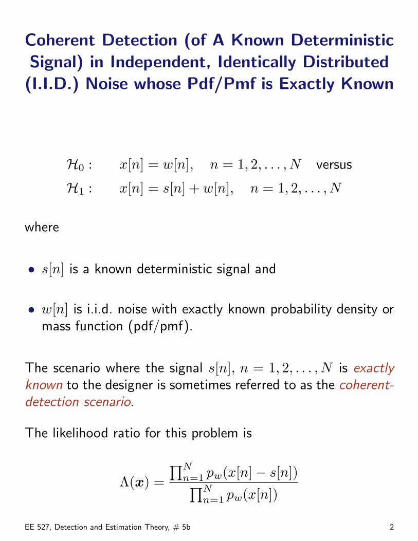
Coherent Detection (of A Known DeterministicSignal) in Independent, Identically Distributed(I.I.D.) Noise whose Pdf/Pmf is Exactly Known

H0 : x[n] = w[n], n = 1, 2, . . . , N versus

H1 : x[n] = s[n] + w[n], n = 1, 2, . . . , N

where

• s[n] is a known deterministic signal and

• w[n] is i.i.d. noise with exactly known probability density ormass function (pdf/pmf).

The scenario where the signal s[n], n = 1, 2, . . . , N is exactlyknown to the designer is sometimes referred to as the coherent-detection scenario.

The likelihood ratio for this problem is

Λ(x) =∏N

n=1 pw(x[n]− s[n])∏Nn=1 pw(x[n])


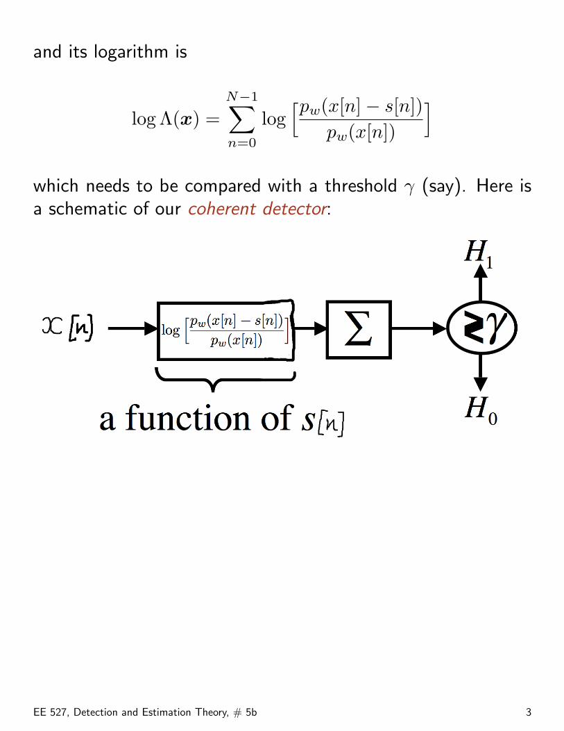
and its logarithm is

log Λ(x) =N−1∑n=0

log[pw(x[n]− s[n])

pw(x[n])

]which needs to be compared with a threshold γ (say). Here isa schematic of our coherent detector:


Example: Coherent Detection in AWGN(Ch. 4 in Kay-II)

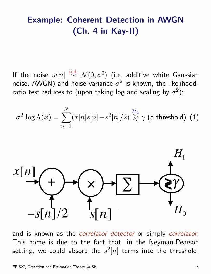
If the noise w[n] i.i.d.∼ N (0, σ2) (i.e. additive white Gaussiannoise, AWGN) and noise variance σ2 is known, the likelihood-ratio test reduces to (upon taking log and scaling by σ2):

σ2 log Λ(x) =N∑

n=1

(x[n]s[n]−s2[n]/2)H1

≷ γ (a threshold) (1)

and is known as the correlator detector or simply correlator.This name is due to the fact that, in the Neyman-Pearsonsetting, we could absorb the s2[n] terms into the threshold,


leading to the test statistic proportional to the samplecorrelation between x[n] and s[n]:

T (x) =N∑

n=1

x[n] s[n]. (2)

We decide H1 if T (x) > γ (the “new” threshold, afterabsorbing the s2[n] terms).

This structure is also known as the matched-filter receiver, dueto the fact that it operates by comparing the output of a linear,time-invariant (LTI) system (filter) to a threshold. Indeed, wecan write (2) as

T (x) =N∑

n=1

x[n] s[n] =∞∑

n=−∞x[n]h[N − n] = {x ? h}[N ]

where {x ? h}[n] denotes convolution of sequences {x[n]} and{h[n]} and, in this case,

h[n] ={

s[N − n], 0 ≤ n ≤ N − 10, otherwise

.

Therefore, this system

• inputs the observation sequence x[1], x[2], . . . , x[N ] to adigital finite impulse response LTI filterand then


• samples the output

y[n] = {x ? h}[n]

at time n = N for comparison with a threshold.

We can express the filter output y[n] in the Fourier domain asfollows:

y[n] =∫ 1/2

−1/2

H(f) X(f) exp(j 2πfn) df

=∫ 1/2

−1/2

[S(f)]∗X(f) exp[j 2πf(n−N)] df

where

H(f) = Fourier transform{s[N − n]}

=N−1∑n=0

s[N − n] exp(−j2πfn)

k=N−n=N∑

k=1

s[k] exp[−j2πf(N − k)]

= exp(−j2πfN) · [S(f)]∗, f ∈ [−12,

12].


Finally, sampling the filter output at n = N yields

T (x) = y[N ] =∫ 1/2

−1/2

[S(f)]∗X(f) df

which is not surprising (recall the Parseval’s theorem).


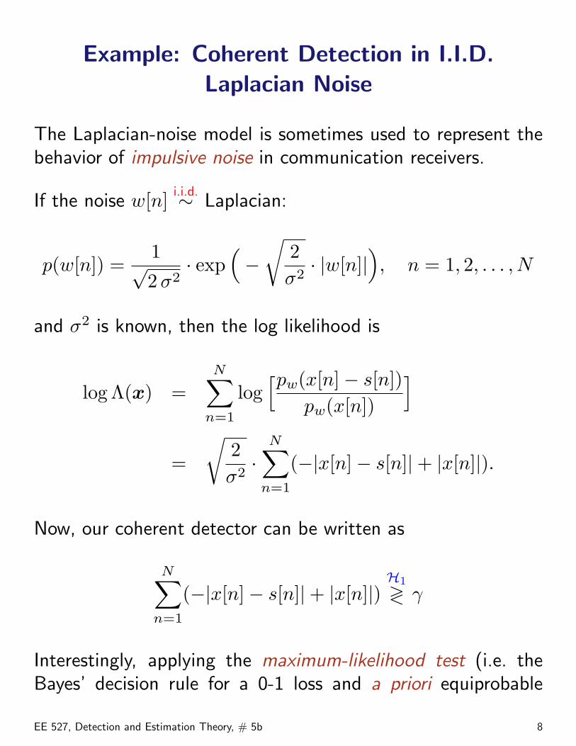
Example: Coherent Detection in I.I.D.Laplacian Noise

The Laplacian-noise model is sometimes used to represent thebehavior of impulsive noise in communication receivers.

If the noise w[n] i.i.d.∼ Laplacian:

p(w[n]) =1√2 σ2

· exp(−√

2σ2· |w[n]|

), n = 1, 2, . . . , N

and σ2 is known, then the log likelihood is

log Λ(x) =N∑

n=1

log[pw(x[n]− s[n])

pw(x[n])

]

=

√2σ2·

N∑n=1

(−|x[n]− s[n]|+ |x[n]|).

Now, our coherent detector can be written as

N∑n=1

(−|x[n]− s[n]|+ |x[n]|)H1

≷ γ

Interestingly, applying the maximum-likelihood test (i.e. theBayes’ decision rule for a 0-1 loss and a priori equiprobable


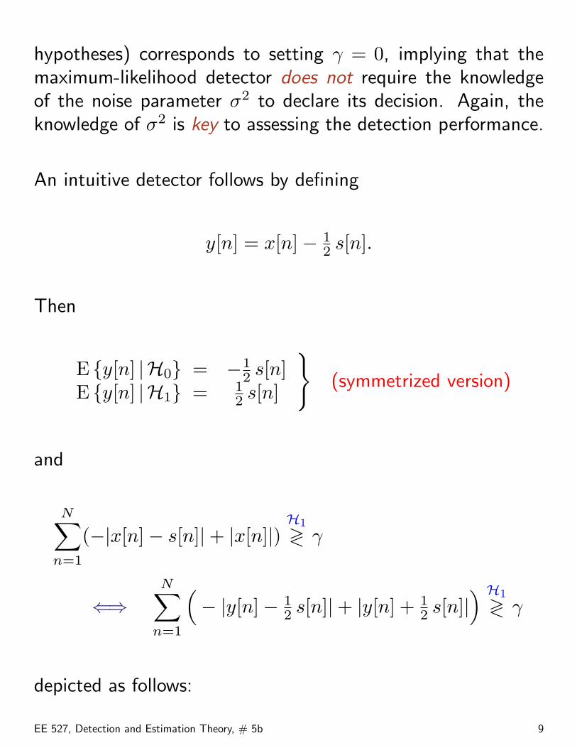
hypotheses) corresponds to setting γ = 0, implying that themaximum-likelihood detector does not require the knowledgeof the noise parameter σ2 to declare its decision. Again, theknowledge of σ2 is key to assessing the detection performance.

An intuitive detector follows by defining

y[n] = x[n]− 12 s[n].

Then

E {y[n] |H0} = −12 s[n]

E {y[n] |H1} = 12 s[n]

}(symmetrized version)

and

N∑n=1

(−|x[n]− s[n]|+ |x[n]|)H1

≷ γ

⇐⇒N∑

n=1

(− |y[n]− 1

2 s[n]|+ |y[n] + 12 s[n]|

) H1

≷ γ

depicted as follows:


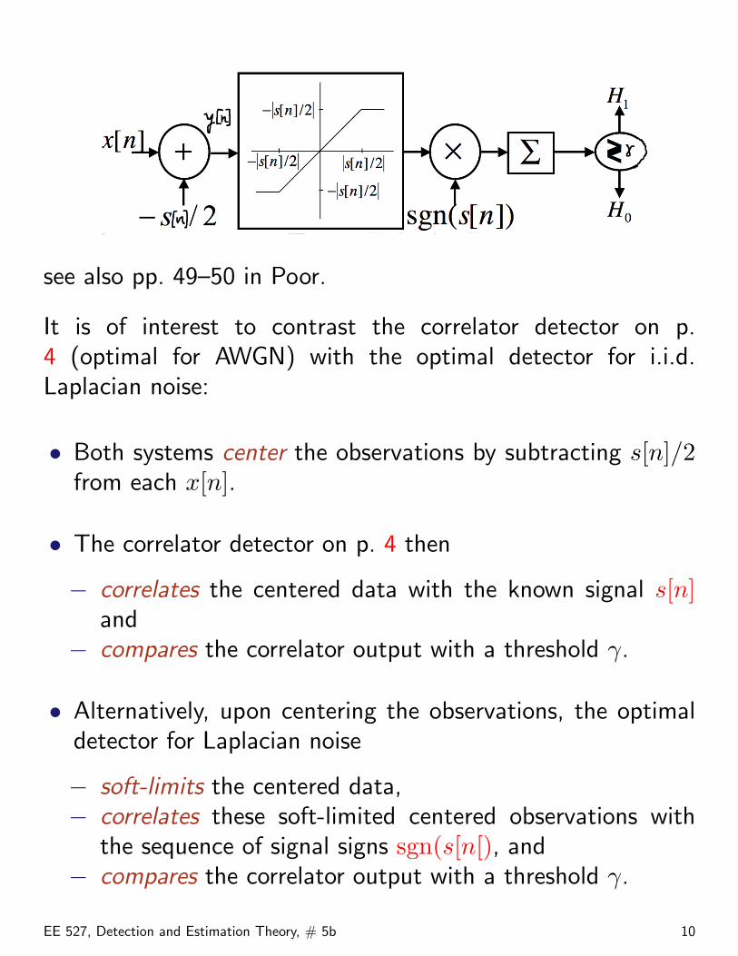
see also pp. 49–50 in Poor.

It is of interest to contrast the correlator detector on p.4 (optimal for AWGN) with the optimal detector for i.i.d.Laplacian noise:

• Both systems center the observations by subtracting s[n]/2from each x[n].

• The correlator detector on p. 4 then

− correlates the centered data with the known signal s[n]and

− compares the correlator output with a threshold γ.

• Alternatively, upon centering the observations, the optimaldetector for Laplacian noise

− soft-limits the centered data,− correlates these soft-limited centered observations with

the sequence of signal signs sgn(s[n[), and− compares the correlator output with a threshold γ.


Soft-limiting in the optimal detector for Laplacian noise reducesthe effect of large observations on the correlator sum and,therefore, makes the system robust to large noise values (whichwill occur frequently due to the heavy tails of the Laplacianpdf).


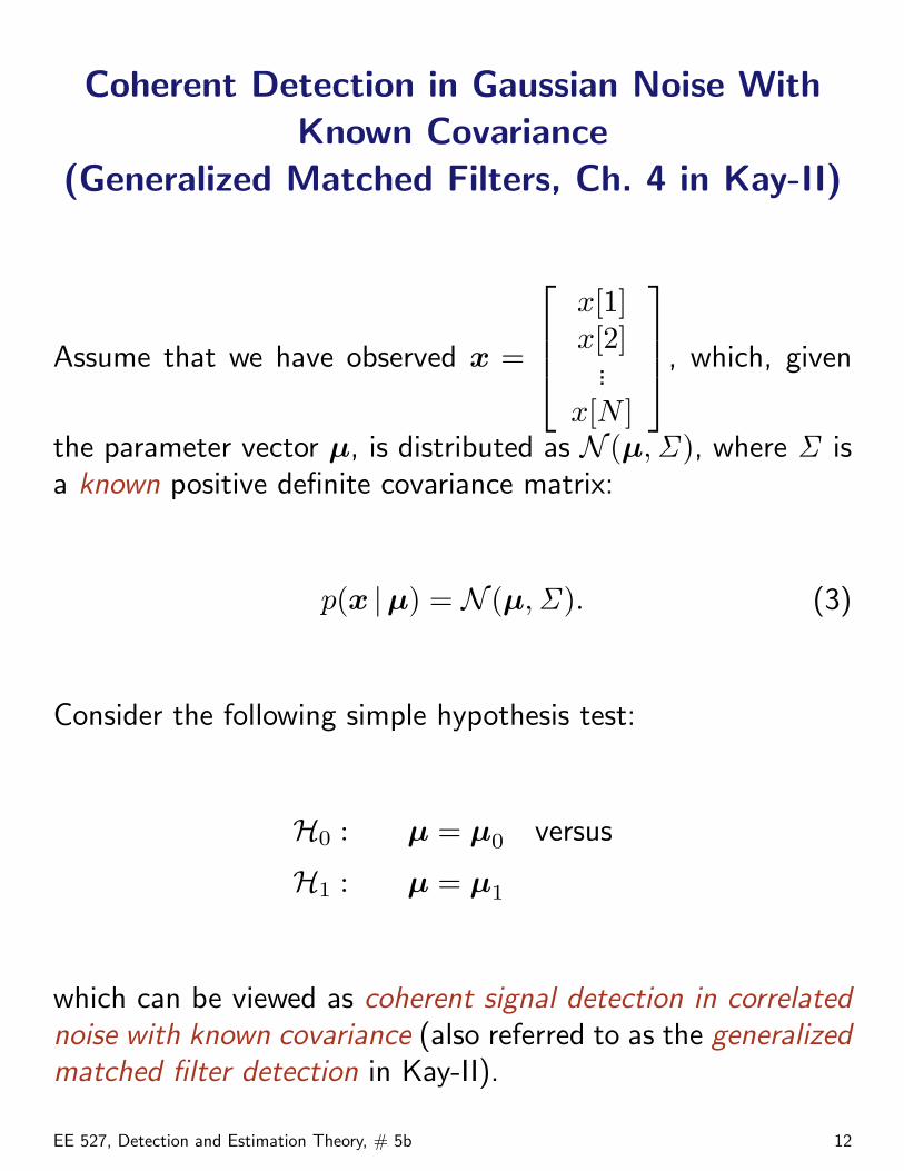
Coherent Detection in Gaussian Noise WithKnown Covariance

(Generalized Matched Filters, Ch. 4 in Kay-II)

Assume that we have observed x =

x[1]x[2]

...x[N ]

, which, given

the parameter vector µ, is distributed as N (µ,Σ ), where Σ isa known positive definite covariance matrix:

p(x |µ) = N (µ,Σ ). (3)

Consider the following simple hypothesis test:

H0 : µ = µ0 versus

H1 : µ = µ1

which can be viewed as coherent signal detection in correlatednoise with known covariance (also referred to as the generalizedmatched filter detection in Kay-II).


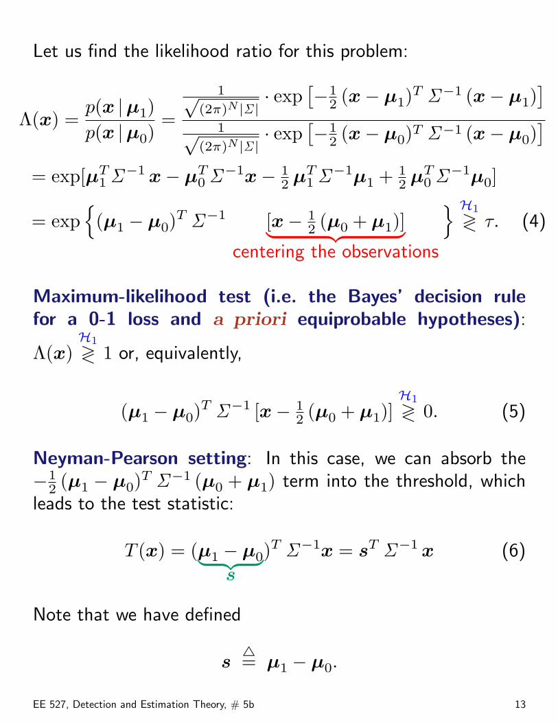
Let us find the likelihood ratio for this problem:

Λ(x) =p(x |µ1)p(x |µ0)

=

1√(2π)N |Σ |

· exp[−1

2 (x− µ1)T Σ−1 (x− µ1)]

1√(2π)N |Σ |

· exp[−1

2 (x− µ0)T Σ−1 (x− µ0)]

= exp[µT1 Σ−1 x− µT

0 Σ−1x− 12 µT

1 Σ−1µ1 + 12 µT

0 Σ−1µ0]

= exp{

(µ1 − µ0)T Σ−1 [x− 1

2 (µ0 + µ1)]︸︷︷︸centering the observations

} H1

≷ τ. (4)

Maximum-likelihood test (i.e. the Bayes’ decision rulefor a 0-1 loss and a priori equiprobable hypotheses):

Λ(x)H1

≷ 1 or, equivalently,

(µ1 − µ0)T Σ−1 [x− 1

2 (µ0 + µ1)]H1

≷ 0. (5)

Neyman-Pearson setting: In this case, we can absorb the−1

2 (µ1 − µ0)T Σ−1 (µ0 + µ1) term into the threshold, whichleads to the test statistic:

T (x) = (µ1 − µ0︸︷︷︸s

)T Σ−1x = sT Σ−1 x (6)

Note that we have defined

s4= µ1 − µ0.


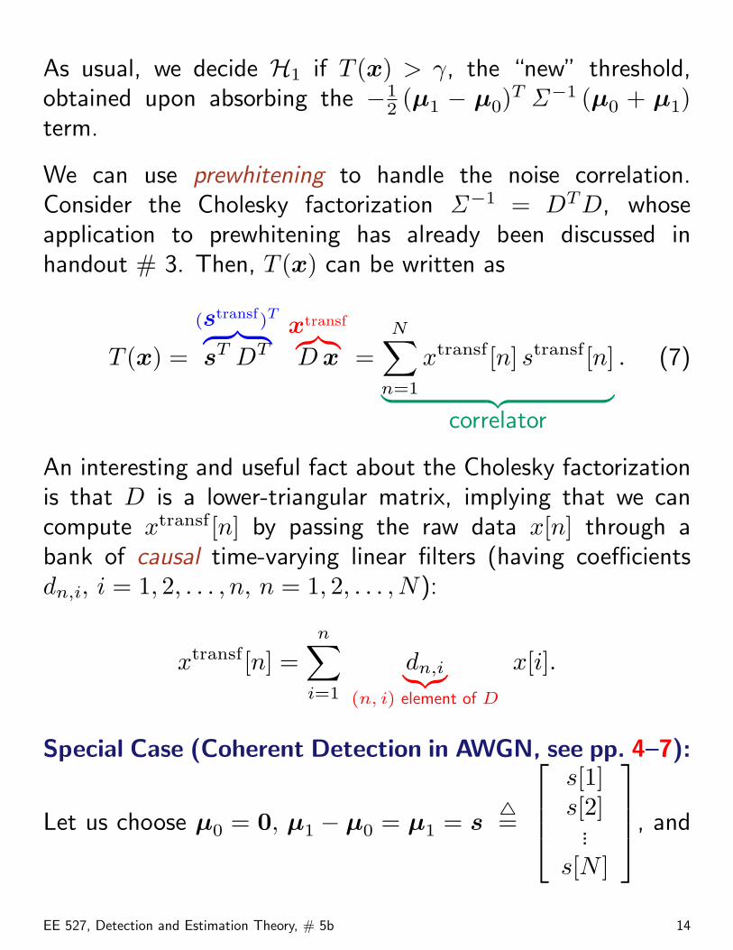
As usual, we decide H1 if T (x) > γ, the “new” threshold,obtained upon absorbing the −1

2 (µ1 − µ0)T Σ−1 (µ0 + µ1)term.

We can use prewhitening to handle the noise correlation.Consider the Cholesky factorization Σ−1 = DTD, whoseapplication to prewhitening has already been discussed inhandout # 3. Then, T (x) can be written as

T (x) =

(stransf)T︷︸︸︷sT DT

xtransf︷︸︸︷D x =

N∑n=1

xtransf[n] stransf[n]︸︷︷︸correlator

. (7)

An interesting and useful fact about the Cholesky factorizationis that D is a lower-triangular matrix, implying that we cancompute xtransf[n] by passing the raw data x[n] through abank of causal time-varying linear filters (having coefficientsdn,i, i = 1, 2, . . . , n, n = 1, 2, . . . , N):

xtransf[n] =n∑

i=1

dn,i︸︷︷︸(n, i) element of D

x[i].

Special Case (Coherent Detection in AWGN, see pp. 4–7):

Let us choose µ0 = 0, µ1 − µ0 = µ1 = s4=

s[1]s[2]...

s[N ]

, and


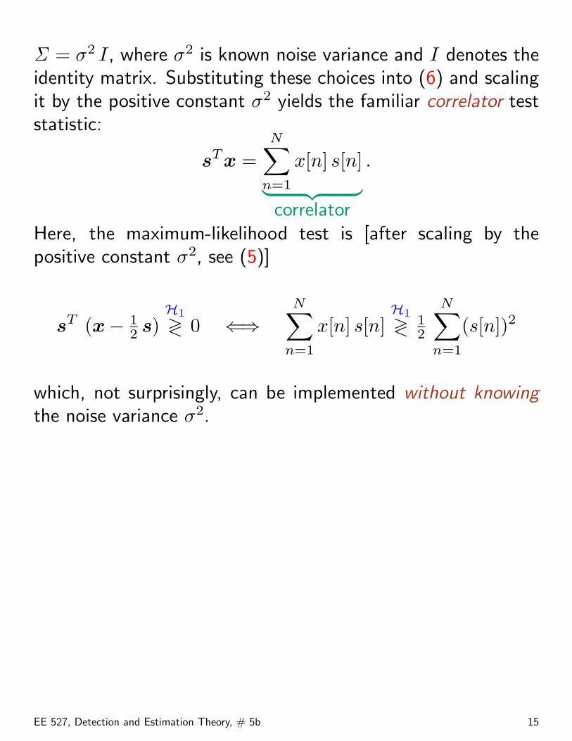
Σ = σ2 I, where σ2 is known noise variance and I denotes theidentity matrix. Substituting these choices into (6) and scalingit by the positive constant σ2 yields the familiar correlator teststatistic:

sTx =N∑

n=1

x[n] s[n]︸︷︷︸correlator

.

Here, the maximum-likelihood test is [after scaling by thepositive constant σ2, see (5)]

sT (x− 12 s)

H1

≷ 0 ⇐⇒N∑

n=1

x[n] s[n]H1

≷ 12

N∑n=1

(s[n])2

which, not surprisingly, can be implemented without knowingthe noise variance σ2.


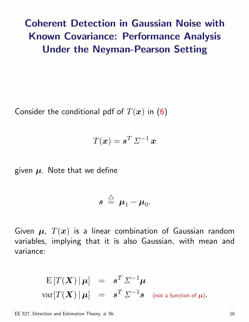
Coherent Detection in Gaussian Noise withKnown Covariance: Performance Analysis

Under the Neyman-Pearson Setting

Consider the conditional pdf of T (x) in (6)

T (x) = sT Σ−1 x

given µ. Note that we define

s4= µ1 − µ0.

Given µ, T (x) is a linear combination of Gaussian randomvariables, implying that it is also Gaussian, with mean andvariance:

E [T (X) |µ] = sT Σ−1µ

var[T (X) |µ] = sT Σ−1s (not a function of µ).


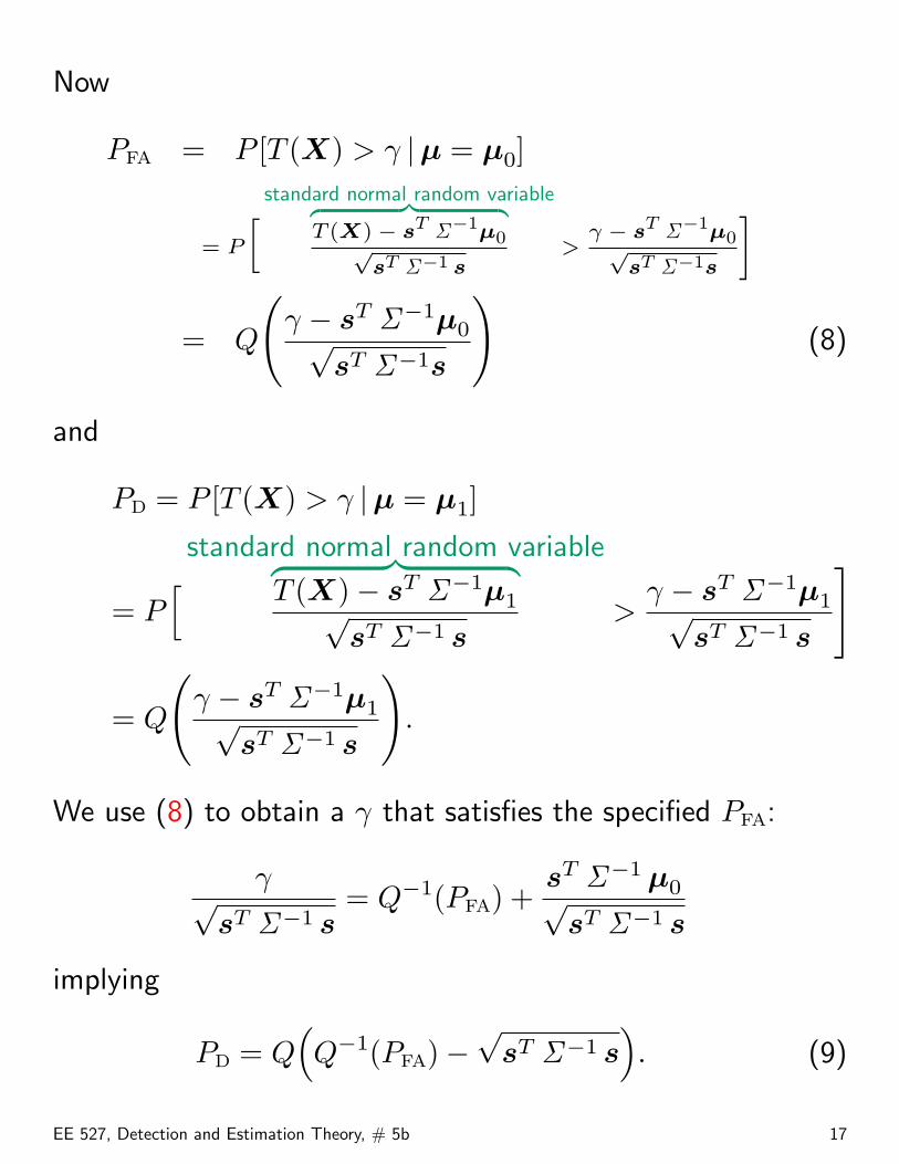
Now

PFA = P [T (X) > γ |µ = µ0]

= P

[ standard normal random variablez }| {T (X)− sT Σ−1µ0√

sT Σ−1 s>

γ − sT Σ−1µ0√sT Σ−1s

#

= Q

(γ − sT Σ−1µ0√

sT Σ−1s

)(8)

and

PD = P [T (X) > γ |µ = µ1]

= P[ standard normal random variable︷︸︸︷

T (X)− sT Σ−1µ1√sT Σ−1 s

>γ − sT Σ−1µ1√

sT Σ−1 s

]

= Q

(γ − sT Σ−1µ1√

sT Σ−1 s

).

We use (8) to obtain a γ that satisfies the specified PFA:

γ√sT Σ−1 s

= Q−1(PFA) +sT Σ−1 µ0√

sT Σ−1 s

implying

PD = Q(Q−1(PFA)−

√sT Σ−1 s

). (9)


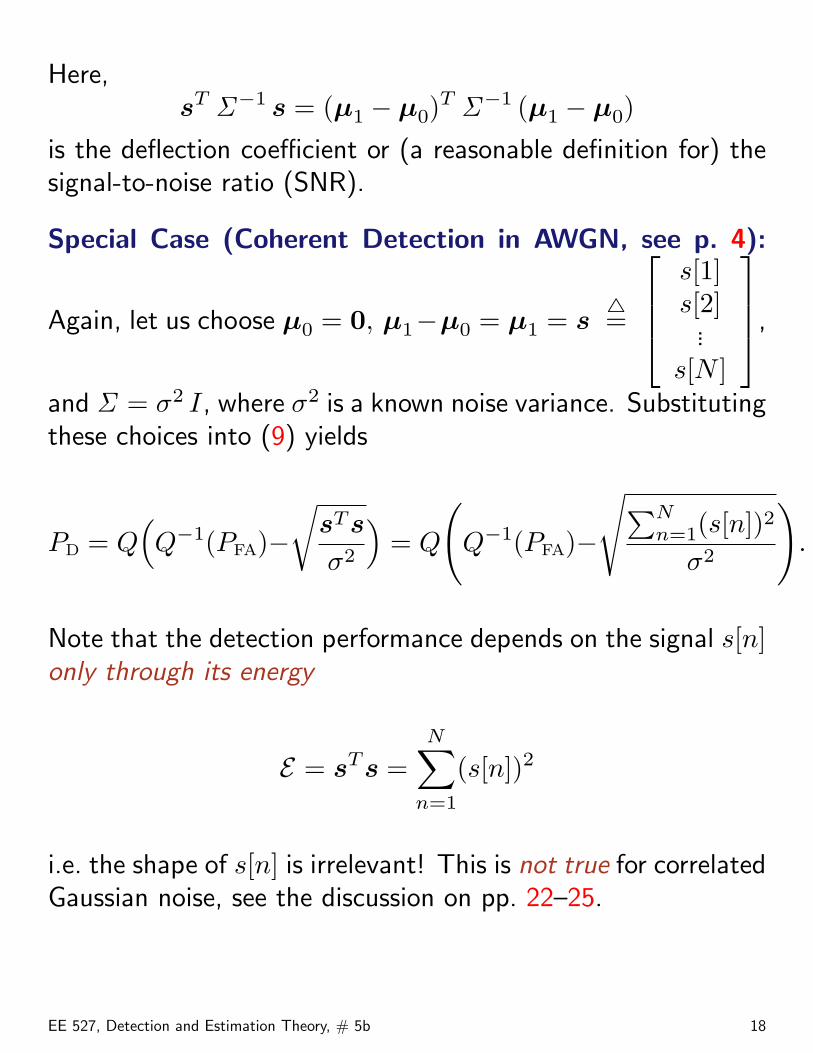
Here,sT Σ−1 s = (µ1 − µ0)

T Σ−1 (µ1 − µ0)

is the deflection coefficient or (a reasonable definition for) thesignal-to-noise ratio (SNR).

Special Case (Coherent Detection in AWGN, see p. 4):

Again, let us choose µ0 = 0, µ1−µ0 = µ1 = s4=

s[1]s[2]...

s[N ]

,

and Σ = σ2 I, where σ2 is a known noise variance. Substitutingthese choices into (9) yields


√sTs

σ2

)= Q

(Q−1(PFA)−

√∑Nn=1(s[n])2

σ2

).

Note that the detection performance depends on the signal s[n]only through its energy

E = sTs =N∑

n=1

(s[n])2

i.e. the shape of s[n] is irrelevant! This is not true for correlatedGaussian noise, see the discussion on pp. 22–25.


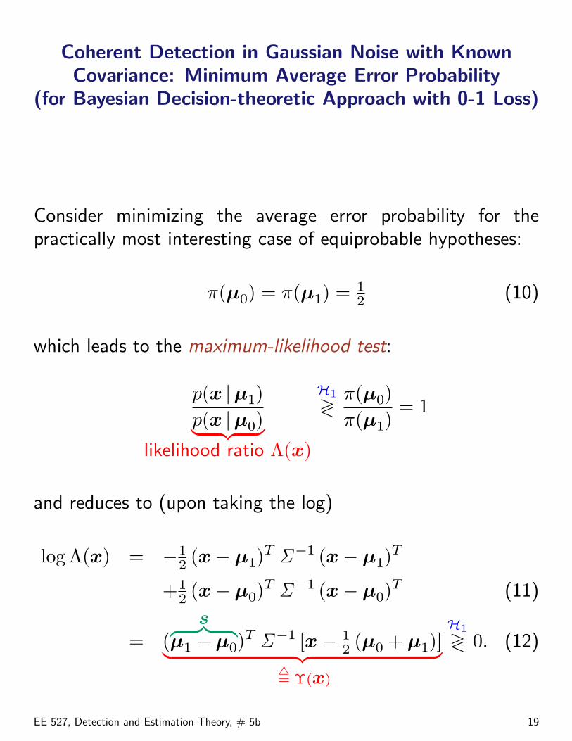
Coherent Detection in Gaussian Noise with KnownCovariance: Minimum Average Error Probability

(for Bayesian Decision-theoretic Approach with 0-1 Loss)

Consider minimizing the average error probability for thepractically most interesting case of equiprobable hypotheses:

π(µ0) = π(µ1) = 12 (10)

which leads to the maximum-likelihood test:

p(x |µ1)p(x |µ0)︸︷︷︸

likelihood ratio Λ(x)

H1

≷π(µ0)π(µ1)

= 1

and reduces to (upon taking the log)

log Λ(x) = −12 (x− µ1)

T Σ−1 (x− µ1)T

+12 (x− µ0)

T Σ−1 (x− µ0)T (11)

= (s︷︸︸︷

µ1 − µ0)T Σ−1 [x− 1

2 (µ0 + µ1)]︸︷︷︸4= Υ(x)

H1

≷ 0. (12)


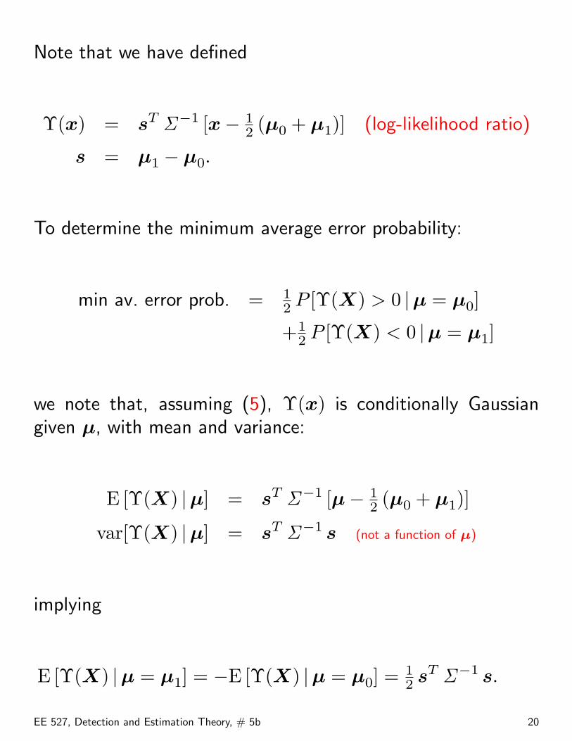
Note that we have defined

Υ(x) = sT Σ−1 [x− 12 (µ0 + µ1)] (log-likelihood ratio)

s = µ1 − µ0.

To determine the minimum average error probability:

min av. error prob. = 12 P [Υ(X) > 0 |µ = µ0]

+12 P [Υ(X) < 0 |µ = µ1]

we note that, assuming (5), Υ(x) is conditionally Gaussiangiven µ, with mean and variance:

E [Υ(X) |µ] = sT Σ−1 [µ− 12 (µ0 + µ1)]

var[Υ(X) |µ] = sT Σ−1 s (not a function of µ)

implying

E [Υ(X) |µ = µ1] = −E [Υ(X) |µ = µ0] = 12 sT Σ−1 s.


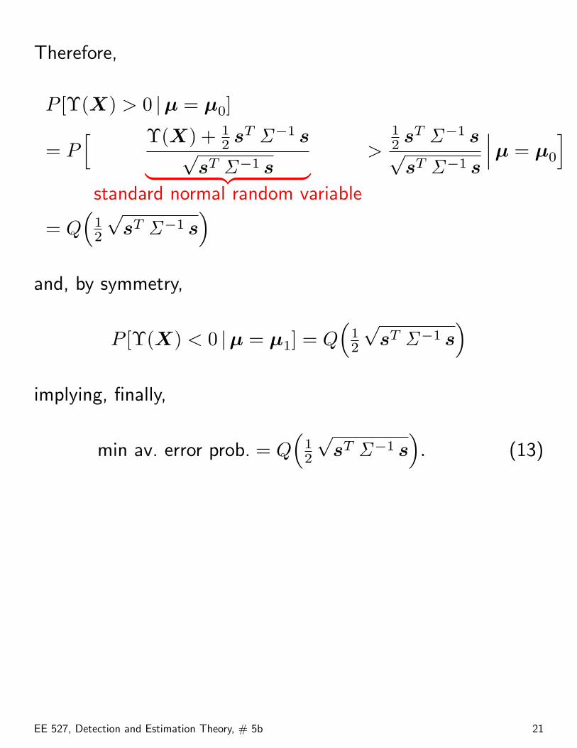
Therefore,

P [Υ(X) > 0 |µ = µ0]

= P[ Υ(X) + 1

2 sT Σ−1 s√

sT Σ−1 s︸︷︷︸standard normal random variable

>12 sT Σ−1 s√

sT Σ−1 s

∣∣∣µ = µ0

]

= Q(

12

√sT Σ−1 s

)and, by symmetry,

P [Υ(X) < 0 |µ = µ1] = Q(

12

√sT Σ−1 s

)implying, finally,

min av. error prob. = Q(

12

√sT Σ−1 s

). (13)


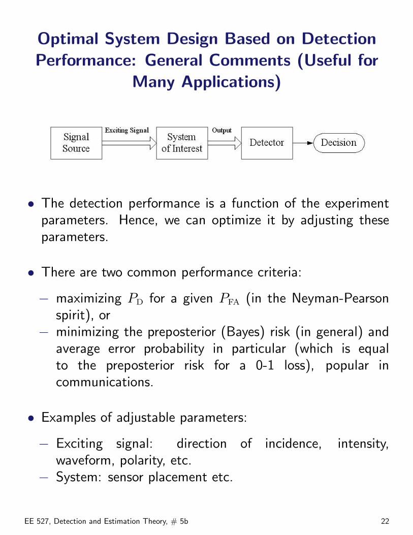
Optimal System Design Based on DetectionPerformance: General Comments (Useful for

Many Applications)

• The detection performance is a function of the experimentparameters. Hence, we can optimize it by adjusting theseparameters.

• There are two common performance criteria:

− maximizing PD for a given PFA (in the Neyman-Pearsonspirit), or

− minimizing the preposterior (Bayes) risk (in general) andaverage error probability in particular (which is equalto the preposterior risk for a 0-1 loss), popular incommunications.

• Examples of adjustable parameters:

− Exciting signal: direction of incidence, intensity,waveform, polarity, etc.

− System: sensor placement etc.


Example: Optimal Signal-waveform Design forCoherent Detection in Correlated Gaussian

Noise with Known Covariance

Consider a coherent radar/sonar/NDE scenario with µ0 = 0,µ1 = s, and correlated Gaussian noise with known covariance.In the Neyman-Pearson spirit, let us maximize PD for a givenPFA. First, recall the expression (9) for the detection probability:


√sT Σ−1 s

).

Note that PD increases monotonically as the deflectioncoefficient sT Σ−1 s grows. Since here larger signal energyclearly improves the detection performance and our focus ison optimizing the signal shape, we now impose the energyconstraint:

sTs = E (E is specified).

Hence, we have the following optimization problem:

maxs

sT Σ−1 s subject to sT s = E

or, (almost) equivalently,

maxs

sT Σ−1 s

sT s=

1mini λi(Σ )


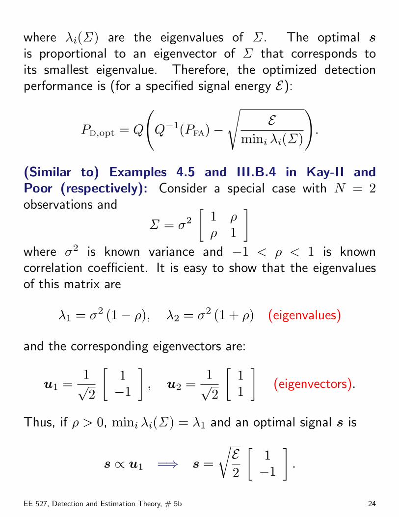
where λi(Σ ) are the eigenvalues of Σ . The optimal sis proportional to an eigenvector of Σ that corresponds toits smallest eigenvalue. Therefore, the optimized detectionperformance is (for a specified signal energy E):

PD,opt = Q

(Q−1(PFA)−

√E

mini λi(Σ )

).

(Similar to) Examples 4.5 and III.B.4 in Kay-II andPoor (respectively): Consider a special case with N = 2observations and

Σ = σ2

[1 ρρ 1

]where σ2 is known variance and −1 < ρ < 1 is knowncorrelation coefficient. It is easy to show that the eigenvaluesof this matrix are

λ1 = σ2 (1− ρ), λ2 = σ2 (1 + ρ) (eigenvalues)

and the corresponding eigenvectors are:

u1 =1√2

[1−1

], u2 =

1√2

[11

](eigenvectors).

Thus, if ρ > 0, mini λi(Σ ) = λ1 and an optimal signal s is

s ∝ u1 =⇒ s =

√E2

[1−1

].


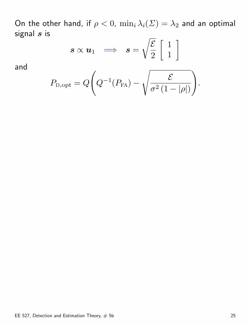
On the other hand, if ρ < 0, mini λi(Σ ) = λ2 and an optimalsignal s is

s ∝ u1 =⇒ s =

√E2

[11

]and

PD,opt = Q

(Q−1(PFA)−

√E

σ2 (1− |ρ|)

).


Two Known Signals in AWGN:Minimum Average-Error ProbabilityApproach to Coherent Detection

(Bayesian Decision Theory for 0-1 Loss)

We first consider the binary case:

H0 : x[n] = s0[n] + w[n], n = 1, 2, . . . , N versus

H1 : x[n] = s1[n] + w[n], n = 1, 2, . . . , N

and the standard AWGN model for w[n]:

w[n] i.i.d.∼ N (0, σ2)

with known variance σ2. This problem fits into our coherentdetection formulation for Gaussian noise:

H0 : µ = µ0 versus

H1 : µ = µ1

with

Σ = σ2 I, µ0 =

s0[1]s0[2]

...s0[N ]

, µ1 =

s1[1]s1[2]

...s1[N ]

. (14)


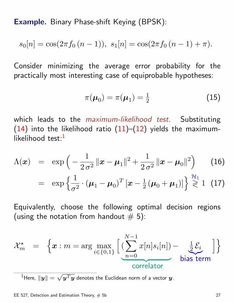
Example. Binary Phase-shift Keying (BPSK):

s0[n] = cos(2πf0 (n− 1)), s1[n] = cos(2πf0 (n− 1) + π).

Consider minimizing the average error probability for thepractically most interesting case of equiprobable hypotheses:

π(µ0) = π(µ1) = 12 (15)

which leads to the maximum-likelihood test. Substituting(14) into the likelihood ratio (11)–(12) yields the maximum-likelihood test:1

Λ(x) = exp(− 1

2 σ2‖x− µ1‖2 +

12 σ2

‖x− µ0‖2)

(16)

= exp{ 1

σ2· (µ1 − µ0)

T [x− 12 (µ0 + µ1)]

} H1

≷ 1 (17)

Equivalently, choose the following optimal decision regions(using the notation from handout # 5):

X ?m =

{x : m = arg max

i∈{0,1}

[(N−1∑n=0

x[n]si[n])︸︷︷︸correlator

− 12 Ei︸︷︷︸

bias term

]}

1Here, ‖y‖ =p

yT y denotes the Euclidean norm of a vector y.


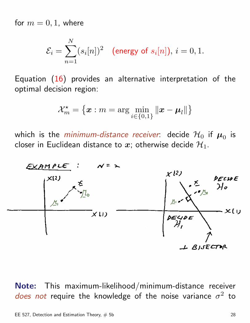
for m = 0, 1, where

Ei =N∑

n=1

(si[n])2 (energy of si[n]), i = 0, 1.

Equation (16) provides an alternative interpretation of theoptimal decision region:

X ?m =

{x : m = arg min

i∈{0,1}‖x− µl‖

}which is the minimum-distance receiver: decide H0 if µ0 iscloser in Euclidean distance to x; otherwise decide H1.

Note: This maximum-likelihood/minimum-distance receiverdoes not require the knowledge of the noise variance σ2 to


make the decision. However, the knowledge of σ2 is key toassessing the error-probability performance of this (and anyother) receiver in AWGN.


If E0 = E1, simply select the hypothesis yielding the largercorrelation:

X ?m =

{x : m = arg max

i∈{0,1}

(N−1∑n=0

x[n]si[n]︸︷︷︸correlator

)}.

Performance Analysis. Substituting (14) into (13) yields

min av. error prob. = Q(

12

‖µ1 − µ0‖σ

)(18)

which has been derived for equiprobable hypotheses (10), seealso the derivation on pp. 19–21. As expected, this minimumaverage error probability decreases as the separation betweenµ1 and µ0 (quantified by ‖µ1 − µ0‖) increases.

Recall that we are focusing on the communication scenario here.Due to the FCC regulations or the physics of the transmittingdevice, we must impose an energy constraint. Let us constrainthe average signal energy [assuming equiprobable hypotheses(10)]:

E = 12 (E0 + E1) (E is specified).

Now

‖µ1 − µ0‖2 = µT1 µ1 − 2µT

1 µ0 + µT0 µ0 = 2 E − 2 µT

1 µ0

= 2 E(1− µT

1 µ0

E

)EE 527, Detection and Estimation Theory, # 5b 30

which suggests the following definition of the signal correlation:

ρs4=

µT1 µ0

E.

Then

‖µ1 − µ0‖2 = 2 E (1− ρs)

and, upon substituting into (18), we obtain

min av. error prob. = Q(√E (1− ρs)

2 σ2

)which is minimized (for a given E) when ρs = −1, i.e. µ1 =−µ0.

Example. BPSK:

s0[n] = cos(2πf0(n− 1)), s1[n] = cos(2πf0(n− 1) + π)

for n = 1, 2, . . . , N . In this case,

µ1 = −µ0 (antipodal signaling)

yielding

ρs = −1


which is the optimal signaling choice that minimizes the averageerror probability, and

min av. error probability = Q(√ E

σ2

).

where

E = E0 = E1 ≈NA2

2.

Therefore, BPSK is the optimal signaling scheme for coherentbinary detection in AWGN with equiprobable hypotheses.

Example. Frequency-shift keying (FSK):

s0[n] = A cos(2πf0(n− 1)

)s1[n] = A cos

(2πf1(n− 1)

), n = 1, 2, . . . , N.

For |f1 − f0| � 1/N , we have

N−1∑n=0

s0[n]s1[n] ≈ 0 i.e. ρs ≈ 0

and

min av. error probability = Q(√ E

2 σ2

)EE 527, Detection and Estimation Theory, # 5b 32

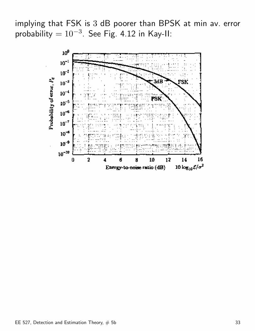
implying that FSK is 3 dB poorer than BPSK at min av. errorprobability = 10−3. See Fig. 4.12 in Kay-II:


Multiple Known Signals in AWGN: MinimumAverage-Error Probability Approach to Coherent

Detection (Bayesian Decision Theory for 0-1 Loss)(Ch. 4.5.3 in Kay-II)

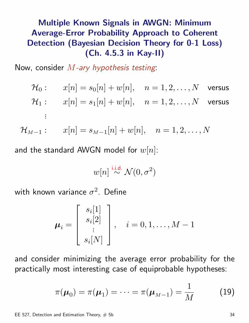
Now, consider M -ary hypothesis testing:



...

HM−1 : x[n] = sM−1[n] + w[n], n = 1, 2, . . . , N

and the standard AWGN model for w[n]:

w[n] i.i.d.∼ N (0, σ2)

with known variance σ2. Define

µi =

si[1]si[2]

...si[N ]

, i = 0, 1, . . . ,M − 1

and consider minimizing the average error probability for thepractically most interesting case of equiprobable hypotheses:

π(µ0) = π(µ1) = · · · = π(µM−1) =1M

(19)


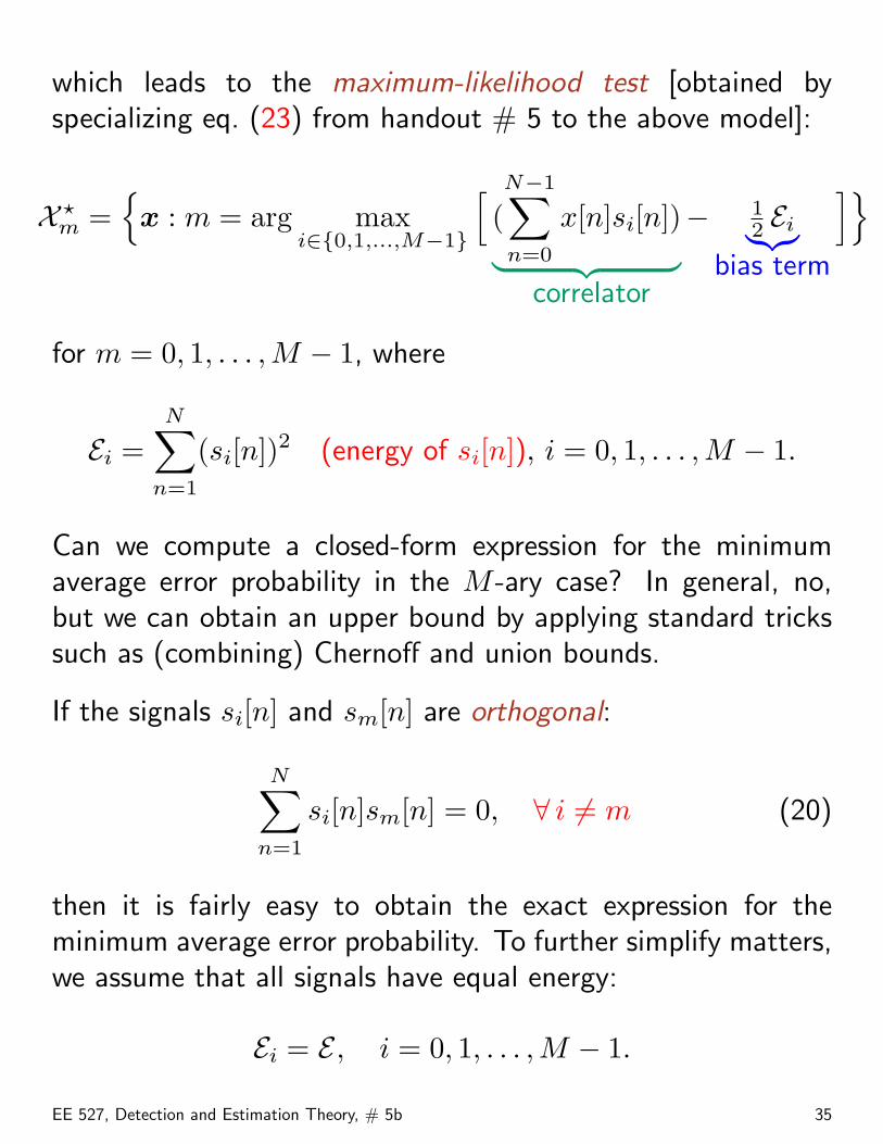
which leads to the maximum-likelihood test [obtained byspecializing eq. (23) from handout # 5 to the above model]:

X ?m =

{x : m = arg max

i∈{0,1,...,M−1}

[(N−1∑n=0

x[n]si[n])︸︷︷︸correlator

− 12 Ei︸︷︷︸

bias term

]}

for m = 0, 1, . . . ,M − 1, where

Ei =N∑

n=1

(si[n])2 (energy of si[n]), i = 0, 1, . . . ,M − 1.

Can we compute a closed-form expression for the minimumaverage error probability in the M -ary case? In general, no,but we can obtain an upper bound by applying standard trickssuch as (combining) Chernoff and union bounds.

If the signals si[n] and sm[n] are orthogonal:

N∑n=1

si[n]sm[n] = 0, ∀ i 6= m (20)

then it is fairly easy to obtain the exact expression for theminimum average error probability. To further simplify matters,we assume that all signals have equal energy:

Ei = E , i = 0, 1, . . . ,M − 1.


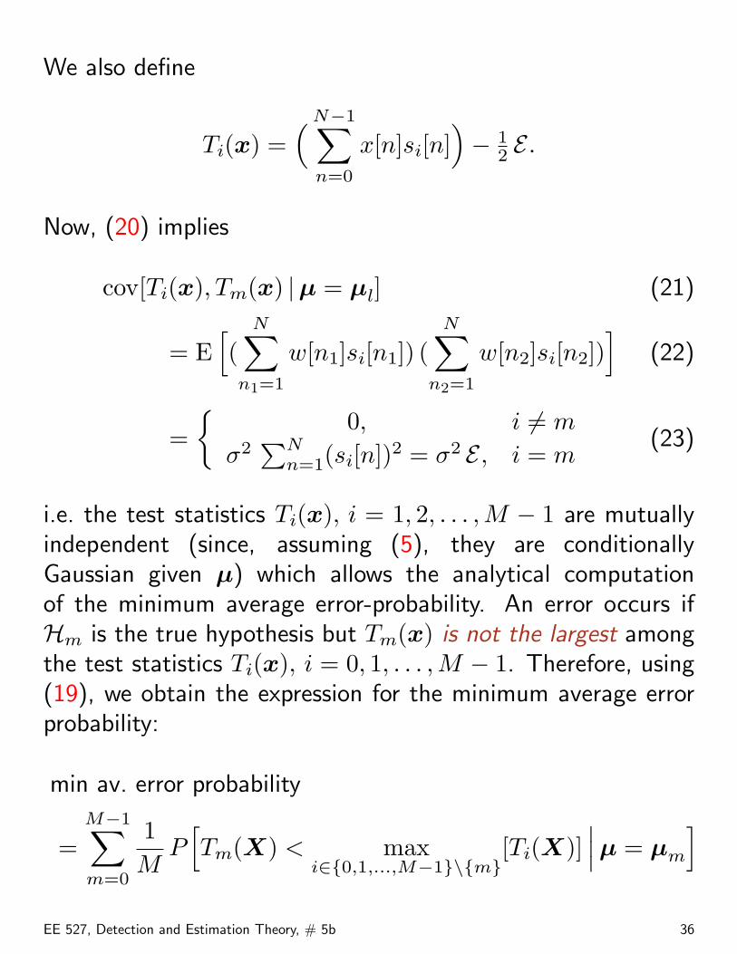
We also define

Ti(x) =(N−1∑

n=0

x[n]si[n])− 1

2 E .

Now, (20) implies

cov[Ti(x), Tm(x) |µ = µl] (21)

= E[(

N∑n1=1

w[n1]si[n1]) (N∑

n2=1

w[n2]si[n2])]

(22)

={

0, i 6= m

σ2∑N

n=1(si[n])2 = σ2 E , i = m(23)

i.e. the test statistics Ti(x), i = 1, 2, . . . ,M − 1 are mutuallyindependent (since, assuming (5), they are conditionallyGaussian given µ) which allows the analytical computationof the minimum average error-probability. An error occurs ifHm is the true hypothesis but Tm(x) is not the largest amongthe test statistics Ti(x), i = 0, 1, . . . ,M − 1. Therefore, using(19), we obtain the expression for the minimum average errorprobability:

min av. error probability

=M−1∑m=0

1M

P[Tm(X) < max

i∈{0,1,...,M−1}\{m}[Ti(X)]

∣∣∣µ = µm

]EE 527, Detection and Estimation Theory, # 5b 36

which simplifies, by symmetry, to a single conditionalprobability:

min av. error prob. = P[T0(X) < max

i∈{1,2,...,M−1}[Ti(X)]

∣∣∣µ = µ0

].

Since Ti(X) are affine functions of Gaussian random variables,they are also Gaussian under H0:

p(Ti(x) |µ = µ0) ={N (1

2 E , σ2 E), i = 0N (0, σ2 E), i 6= 0

and thus [using independence in (23), which is critical fortractability]


= 1− P[T0(X) > max

i∈{1,2,...,M−1}[Ti(X)]

∣∣∣µ = µ0

]= 1− P

[T0(X) > T1(X), T0(X) > T2(X),

. . . , T0(X) > TM(X)∣∣∣µ = µ0

]total. prob.

= 1

−Z

P[t0 > T1(X), t0 > T2(X), . . . , t0 > TM(X)

˛̨̨T0(x) = t0, µ = µ0

ipT0

(t0) dt0

independence= 1−

∫ ∞

−∞

{M−1∏i=1

P [Ti(X) < t0 |µ = µ0]}

pT0(t0) dt0


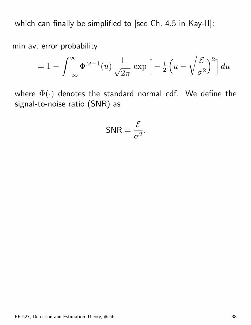
which can finally be simplified to [see Ch. 4.5 in Kay-II]:


= 1−∫ ∞

−∞ΦM−1(u)

1√2π

exp[− 1

2

(u−

√Eσ2

)2]du

where Φ(·) denotes the standard normal cdf. We define thesignal-to-noise ratio (SNR) as

SNR =Eσ2

.


Coherent Detection - Electrical and Computer …namrata/EE527_Spring08/l5b.pdfknown to the designer...

Documents

Transcript of Coherent Detection - Electrical and Computer …namrata/EE527_Spring08/l5b.pdfknown to the designer...