PCMI 2017 - Introduction to Random Matrix TheoryHandout #2 – 06.27.2017

REVIEW OF PROBABILITY THEORY

Chapter 1 - Events and Their Probabilities

1.1. Events as Sets

Definition (σ-field). A collection F of subsets of Ω is called a σ-field if it satisfies thefollowing conditions:

a) ∅ ∈ F ;

b) If A1, A2, . . . ∈ F then⋃∞i=1 Ai ∈ F ;

c) If A ∈ F then AC ∈ F .

Examples. A few examples of σ-fields associated with Ω:

a) F1 = ∅,Ωb) F2 = ∅, A,AC,Ω, where A is any subset of Ω

c) F3 = 0, 1Ω = A,A ⊂ Ω

With any experiment we may associate a pair (Ω,F), where Ω is the sample space(i.e., the set of all the possible outcomes or elementary events) and F is a σ-field ofsubsets of Ω which contains all the events in whose occurrences we may be interested.

Therefore, to call a set A an event is equivalent to asserting that A belongs to theσ-field in question. We usually translate statements about combinations of events intoset-theoretic jargon.

1.2. Probability

Definition (Probability Measure). A probability measure P on the σ-field (Ω,F) isa function P : F → [0, 1] satisfying

a) P(∅) = 0, P(Ω) = 1;

b) If A1, A2, A3, . . . are disjoint members of F (i.e. Ai ∩ Aj = ∅ for all pairs (i, j),satisfying i 6= j) then

P

(∞⋃i=1

Ai

)=∞∑i=1

P(Ai)

1

Remark. The probability measure P is a function which associates to any event a realnumber between 0 and 1.

Definition (Probability Space). A triple (Ω,F ,P), consisting of a set Ω, a σ-field Fof subsets of Ω, and a probability measure P on (Ω,F), is called a probability space.

Proposition (De Morgan’s Laws). Let Aii∈I be a collection of sets (all subsets ofa set Ω). Then: (⋃

i∈I

Ai

)C

=⋂i∈I

ACi

(⋂i∈I

Ai

)C

=⋃i∈I

ACi

(the complements are taken with respect to the set Ω)

Proposition (Basic Properties of Probability Spaces). Consider the probabilityspace (Ω,F ,P) and let A,B ∈ F . Then

a) P(AC) = 1− P(A)

b) If A ⊆ B then P(B) = P(A) + P(B \ A). Also P(B) ≥ P(A).

c) P(A ∪B) = P(A) + P(B)− P(A ∩B)

d) More generally, if A1, A2, . . . , An are members of F , then

P

(n⋃i=1

Ai

)=

n∑i=1

P(Ai)−∑

1≤i,j≤n, i<j

P(Ai ∩ Aj) +∑

1≤i,j,k≤n, i<j<k

P(Ai ∩ Aj ∩ Ak)− · · ·

+ (−1)n+1P(A1 ∩ A2 ∩ · · · ∩ An)

where, for example,∑

1≤i,j≤n, i<j

P(Ai ∩Aj) sums over all unordered pairs (i, j) with i 6= j.

Proposition (Properties of Increasing/Decreasing Sequences of Events). Con-sider the probability space (Ω,F ,P).

a) If A1 ⊆ A2 ⊆ A3 ⊆ · · · is an increasing sequence of events and A =⋃∞i=1Ai, then

P(A) = limi→∞ P(Ai).

b) If B1 ⊇ B2 ⊇ B3 ⊇ · · · is a decreasing sequence of events and B =⋂∞i=1Bi, then

P(B) = limi→∞ P(Bi).

Definition (Null Event). Consider the probability space (Ω,F ,P). The event A ∈ Fis called null if P(A) = 0.

2

Remarks. The event ∅ is called the impossible event and is a null event (since P(∅) = 0).However, there exist null events that are not the impossible event.

Definition (Almost Sure Event). Consider the probability space (Ω,F ,P). The eventA ∈ F is called almost sure if P(A) = 1.

Remarks. The event Ω is called the certain event and is an almost sure event (sinceP(Ω) = 1). However, there exist almost sure events that are not the certain event.

1.3. Conditional Probability

Definition (Conditional Probability). Consider the probability space (Ω,F ,P) andlet A,B ∈ F . If P(B) > 0 then the probability that the event A occurs given that Boccurs is defined to be

P(A |B) =P(A ∩B)

P(B)

Definition (Partition of a set Ω). Consider the probability space (Ω,F ,P). A familyB1, B2, . . . , Bn of events is called a partition of the set Ω if

a) Bi ∩Bj = ∅ for all pairs (i, j), satisfying i 6= j

b)⋃ni=1 Bi = Ω

Remark. Each elementary event ω ∈ Ω belongs to exactly one set in a partition of Ω.

Proposition (Conditional Probabilities Using Partitions). In the probabilityspace (Ω,F ,P) consider the events A,B ∈ F with 0 < P(B) < 1. Then

P(A) = P(A |B)P(B) + P(A |BC)P(BC)

More generally, if the events B1, B2, . . . , Bn form a partition of Ω such that P(Bi) > 0for all i, we have

P(A) =n∑i=1

P(A |Bi)P(Bi)

Example:

With any random experiment we may associate a probability space, which is a triple(Ω,F ,P), where:• Ω is the sample space (all the possible outcomes)

3

• F is a σ-field of subsets of Ω (all the possible events considered)• P is the probability measure, which is a function P : F → [0, 1]. It associates to any

event A ∈ F its probability, which is a real number between 0 and 1.

Important Special Case: We often consider experiments with finitely many possible out-comes and we assume that all the outcomes are equally likely. In this case, we considerthe probability space (Ω,F ,P), where• Ω = the set of all possible outcomes• F = the collection of all the subsets of Ω

• P : F → [0, 1], P(A) =|A||Ω|

for any A ∈ F (therefore, for any A ⊆ Ω)

(|S| denotes the number of elements of a set S)

Remark: In this Special Case, Ω and F are finite sets and |F| = 2|Ω|.

Special Case - Concrete Example: Consider rolling a fair die. Then we consider theprobability space (Ω,F ,P), where• Ω = 1, 2, 3, 4, 5, 6. Note that |Ω| = 6.

• F =∅,

1, 2, 3, 4 , 5, 6,1, 2, 1, 3, 1, 4, 1, 5, 1, 6, 2, 3, 2, 4, 2, 5, 2, 6, 3, 4, 3, 5,

3, 6, 4, 5, 4, 6, 5, 6,1, 2, 3, 1, 2, 4, 1, 2, 5, 1, 2, 6, 1, 3, 4, 1, 3, 5, 1, 3, 6, 1, 4, 5, 1, 4, 6,

1, 5, 6, 2, 3, 4, 2, 3, 5, 2, 3, 6, 2, 4, 5, 2, 4, 6, 2, 5, 6, 3, 4, 5, 3, 4, 6, 3, 5, 6,4, 5, 6

1, 2, 3, 4, 1, 2, 3, 5, 1, 2, 3, 6, 1, 2, 4, 5, 1, 2, 4, 6, 1, 2, 5, 6, 1, 3, 4, 5,1, 3, 4, 6, 1, 3, 5, 6, 1, 4, 5, 6, 2, 3, 4, 5, 2, 3, 4, 6, 2, 3, 5, 6, , 2, 4, 5, 6, 3, 4, 5, 6

1, 2, 3, 4, 5, 1, 2, 3, 4, 6, 1, 2, 3, 5, 6, 1, 2, 4, 5, 6, 1, 3, 4, 5, 6, 2, 3, 4, 5, 61, 2, 3, 4, 5, 6

• P : F → [0, 1], P(A) =

|A||Ω|

=|A|6

for any A ∈ F

In particular, if A = 2, 4, 6 (the event “the number rolled is even”), then

P(A) =|2, 4, 6|

6=

3

6=

1

2

Useful Results from Combinatorics

1. [Simple Permutations] The number of possible orderings (permutations) of n distinctobjects is n! = 1 · 2 · 3 · · · (n− 1) · n

4

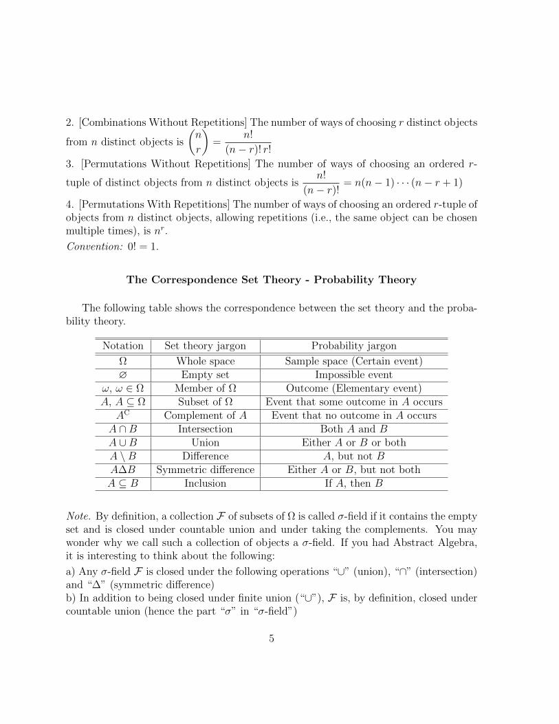
2. [Combinations Without Repetitions] The number of ways of choosing r distinct objects

from n distinct objects is

(n

r

)=

n!

(n− r)! r!3. [Permutations Without Repetitions] The number of ways of choosing an ordered r-

tuple of distinct objects from n distinct objects isn!

(n− r)!= n(n− 1) · · · (n− r + 1)

4. [Permutations With Repetitions] The number of ways of choosing an ordered r-tuple ofobjects from n distinct objects, allowing repetitions (i.e., the same object can be chosenmultiple times), is nr.

Convention: 0! = 1.

The Correspondence Set Theory - Probability Theory

The following table shows the correspondence between the set theory and the proba-bility theory.

Notation Set theory jargon Probability jargon

Ω Whole space Sample space (Certain event)∅ Empty set Impossible event

ω, ω ∈ Ω Member of Ω Outcome (Elementary event)A, A ⊆ Ω Subset of Ω Event that some outcome in A occurs

AC Complement of A Event that no outcome in A occursA ∩B Intersection Both A and BA ∪B Union Either A or B or bothA \B Difference A, but not BA∆B Symmetric difference Either A or B, but not bothA ⊆ B Inclusion If A, then B

Note. By definition, a collection F of subsets of Ω is called σ-field if it contains the emptyset and is closed under countable union and under taking the complements. You maywonder why we call such a collection of objects a σ-field. If you had Abstract Algebra,it is interesting to think about the following:

a) Any σ-field F is closed under the following operations “∪” (union), “∩” (intersection)and “∆” (symmetric difference)b) In addition to being closed under finite union (“∪”), F is, by definition, closed undercountable union (hence the part “σ” in “σ-field”)

5

c) ∅ is identity for the operation “∪” (union); Ω is identity for the operation “∩” (inter-section); ∅ is identity for the operation “∆” (symmetric difference).d) (F ,∆) is an Abelian group (“∆” is the group operation).e) (F ,∆,∩) is a commutative ring (“∆” is the first operation, “∩” is the second opera-tion).

Chapter 2 - Random Variables

2.1. Definitions and Basic Properties

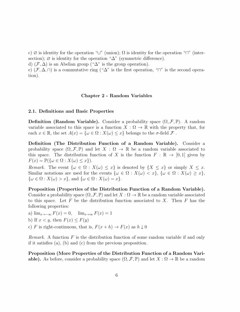
Definition (Random Variable). Consider a probability space (Ω,F ,P). A randomvariable associated to this space is a function X : Ω → R with the property that, foreach x ∈ R, the set A(x) = ω ∈ Ω : X(ω) ≤ x belongs to the σ-field F .

Definition (The Distribution Function of a Random Variable). Consider aprobability space (Ω,F ,P) and let X : Ω → R be a random variable associated tothis space. The distribution function of X is the function F : R → [0, 1] given byF (x) = P(ω ∈ Ω : X(ω) ≤ x).Remark. The event ω ∈ Ω : X(ω) ≤ x is denoted by X ≤ x or simply X ≤ x.Similar notations are used for the events ω ∈ Ω : X(ω) < x, ω ∈ Ω : X(ω) ≥ x,ω ∈ Ω : X(ω) > x, and ω ∈ Ω : X(ω) = x.

Proposition (Properties of the Distribution Function of a Random Variable).Consider a probability space (Ω,F ,P) and let X : Ω→ R be a random variable associatedto this space. Let F be the distribution function associated to X. Then F has thefollowing properties:

a) limx→−∞ F (x) = 0, limx→∞ F (x) = 1

b) If x < y, then F (x) ≤ F (y)

c) F is right-continuous, that is, F (x+ h)→ F (x) as h ↓ 0

Remark. A function F is the distribution function of some random variable if and onlyif it satisfies (a), (b) and (c) from the previous proposition.

Proposition (More Properties of the Distribution Function of a Random Vari-able). As before, consider a probability space (Ω,F ,P) and let X : Ω→ R be a random

6

variable associated to this space. Let F be the distribution function associated to X.Then F has the following properties:

a) P(X > x) = 1− F (x)

b) P(x < X ≤ y) = F (y)− F (x)

c) P(X = x) = F (x)− limy↑x F (y)

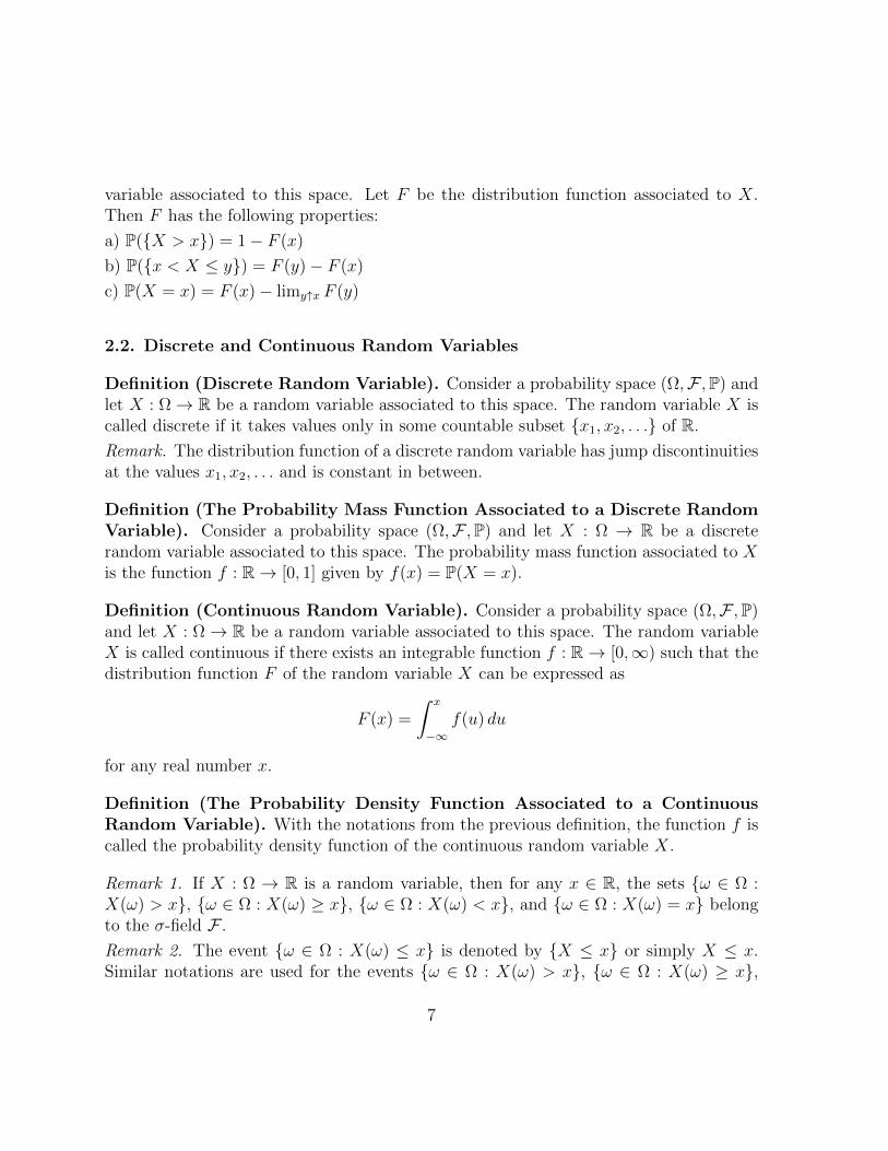
2.2. Discrete and Continuous Random Variables

Definition (Discrete Random Variable). Consider a probability space (Ω,F ,P) andlet X : Ω→ R be a random variable associated to this space. The random variable X iscalled discrete if it takes values only in some countable subset x1, x2, . . . of R.

Remark. The distribution function of a discrete random variable has jump discontinuitiesat the values x1, x2, . . . and is constant in between.

Definition (The Probability Mass Function Associated to a Discrete RandomVariable). Consider a probability space (Ω,F ,P) and let X : Ω → R be a discreterandom variable associated to this space. The probability mass function associated to Xis the function f : R→ [0, 1] given by f(x) = P(X = x).

Definition (Continuous Random Variable). Consider a probability space (Ω,F ,P)and let X : Ω→ R be a random variable associated to this space. The random variableX is called continuous if there exists an integrable function f : R→ [0,∞) such that thedistribution function F of the random variable X can be expressed as

F (x) =

∫ x

−∞f(u) du

for any real number x.

Definition (The Probability Density Function Associated to a ContinuousRandom Variable). With the notations from the previous definition, the function f iscalled the probability density function of the continuous random variable X.

Remark 1. If X : Ω → R is a random variable, then for any x ∈ R, the sets ω ∈ Ω :X(ω) > x, ω ∈ Ω : X(ω) ≥ x, ω ∈ Ω : X(ω) < x, and ω ∈ Ω : X(ω) = x belongto the σ-field F .

Remark 2. The event ω ∈ Ω : X(ω) ≤ x is denoted by X ≤ x or simply X ≤ x.Similar notations are used for the events ω ∈ Ω : X(ω) > x, ω ∈ Ω : X(ω) ≥ x,

7

ω ∈ Ω : X(ω) < x, and ω ∈ Ω : X(ω) = x: X > x, X ≥ x, X < x, andX = x.

Examples of Random Variables and Their Distribution Functions.

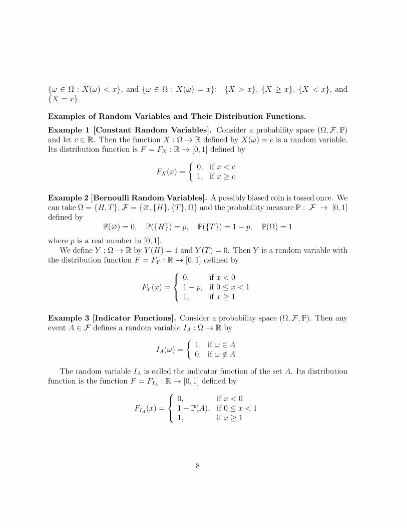
Example 1 [Constant Random Variables]. Consider a probability space (Ω,F ,P)and let c ∈ R. Then the function X : Ω→ R defined by X(ω) = c is a random variable.Its distribution function is F = FX : R→ [0, 1] defined by

FX(x) =

0, if x < c1, if x ≥ c

Example 2 [Bernoulli Random Variables]. A possibly biased coin is tossed once. Wecan take Ω = H,T, F = ∅, H, T,Ω and the probability measure P : F → [0, 1]defined by

P(∅) = 0, P(H) = p, P(T) = 1− p, P(Ω) = 1

where p is a real number in [0, 1].We define Y : Ω→ R by Y (H) = 1 and Y (T ) = 0. Then Y is a random variable with

the distribution function F = FY : R→ [0, 1] defined by

FY (x) =

0, if x < 01− p, if 0 ≤ x < 11, if x ≥ 1

Example 3 [Indicator Functions]. Consider a probability space (Ω,F ,P). Then anyevent A ∈ F defines a random variable IA : Ω→ R by

IA(ω) =

1, if ω ∈ A0, if ω /∈ A

The random variable IA is called the indicator function of the set A. Its distributionfunction is the function F = FIA : R→ [0, 1] defined by

FIA(x) =

0, if x < 01− P(A), if 0 ≤ x < 11, if x ≥ 1

8

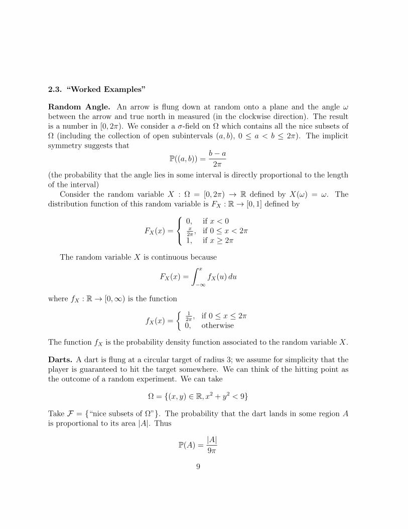
2.3. “Worked Examples”

Random Angle. An arrow is flung down at random onto a plane and the angle ωbetween the arrow and true north in measured (in the clockwise direction). The resultis a number in [0, 2π). We consider a σ-field on Ω which contains all the nice subsets ofΩ (including the collection of open subintervals (a, b), 0 ≤ a < b ≤ 2π). The implicitsymmetry suggests that

P((a, b)) =b− a2π

(the probability that the angle lies in some interval is directly proportional to the lengthof the interval)

Consider the random variable X : Ω = [0, 2π) → R defined by X(ω) = ω. Thedistribution function of this random variable is FX : R→ [0, 1] defined by

FX(x) =

0, if x < 0x2π, if 0 ≤ x < 2π

1, if x ≥ 2π

The random variable X is continuous because

FX(x) =

∫ x

−∞fX(u) du

where fX : R→ [0,∞) is the function

fX(x) =

1

2π, if 0 ≤ x ≤ 2π

0, otherwise

The function fX is the probability density function associated to the random variable X.

Darts. A dart is flung at a circular target of radius 3; we assume for simplicity that theplayer is guaranteed to hit the target somewhere. We can think of the hitting point asthe outcome of a random experiment. We can take

Ω = (x, y) ∈ R, x2 + y2 < 9

Take F = “nice subsets of Ω”. The probability that the dart lands in some region Ais proportional to its area |A|. Thus

P(A) =|A|9π

9

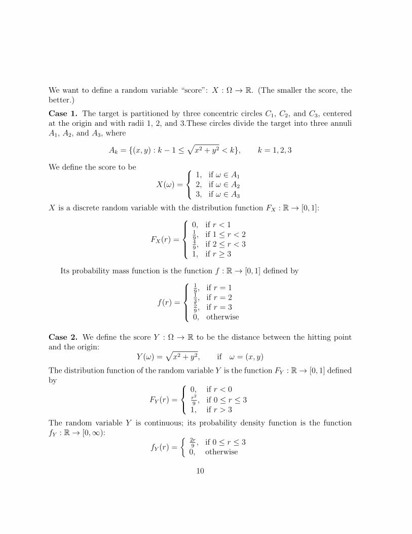
We want to define a random variable “score”: X : Ω → R. (The smaller the score, thebetter.)

Case 1. The target is partitioned by three concentric circles C1, C2, and C3, centeredat the origin and with radii 1, 2, and 3.These circles divide the target into three annuliA1, A2, and A3, where

Ak = (x, y) : k − 1 ≤√x2 + y2 < k, k = 1, 2, 3

We define the score to be

X(ω) =

1, if ω ∈ A1

2, if ω ∈ A2

3, if ω ∈ A3

X is a discrete random variable with the distribution function FX : R→ [0, 1]:

FX(r) =

0, if r < 119, if 1 ≤ r < 2

49, if 2 ≤ r < 3

1, if r ≥ 3

Its probability mass function is the function f : R→ [0, 1] defined by

f(r) =

19, if r = 1

13, if r = 2

59, if r = 3

0, otherwise

Case 2. We define the score Y : Ω → R to be the distance between the hitting pointand the origin:

Y (ω) =√x2 + y2, if ω = (x, y)

The distribution function of the random variable Y is the function FY : R→ [0, 1] definedby

FY (r) =

0, if r < 0r2

9, if 0 ≤ r ≤ 3

1, if r > 3

The random variable Y is continuous; its probability density function is the functionfY : R→ [0,∞):

fY (r) =

2r9, if 0 ≤ r ≤ 3

0, otherwise

10

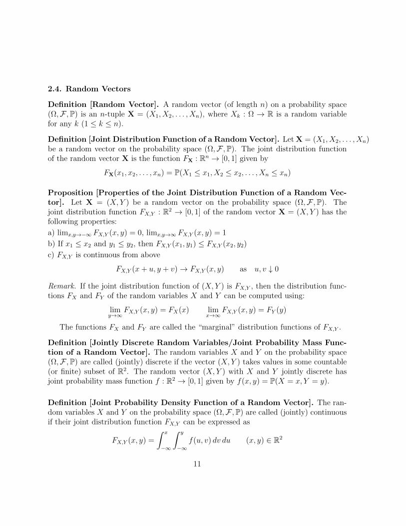
2.4. Random Vectors

Definition [Random Vector]. A random vector (of length n) on a probability space(Ω,F ,P) is an n-tuple X = (X1, X2, . . . , Xn), where Xk : Ω → R is a random variablefor any k (1 ≤ k ≤ n).

Definition [Joint Distribution Function of a Random Vector]. Let X = (X1, X2, . . . , Xn)be a random vector on the probability space (Ω,F ,P). The joint distribution functionof the random vector X is the function FX : Rn → [0, 1] given by

FX(x1, x2, . . . , xn) = P(X1 ≤ x1, X2 ≤ x2, . . . , Xn ≤ xn)

Proposition [Properties of the Joint Distribution Function of a Random Vec-tor]. Let X = (X, Y ) be a random vector on the probability space (Ω,F ,P). Thejoint distribution function FX,Y : R2 → [0, 1] of the random vector X = (X, Y ) has thefollowing properties:

a) limx,y→−∞ FX,Y (x, y) = 0, limx,y→∞ FX,Y (x, y) = 1

b) If x1 ≤ x2 and y1 ≤ y2, then FX,Y (x1, y1) ≤ FX,Y (x2, y2)

c) FX,Y is continuous from above

FX,Y (x+ u, y + v)→ FX,Y (x, y) as u, v ↓ 0

Remark. If the joint distribution function of (X, Y ) is FX,Y , then the distribution func-tions FX and FY of the random variables X and Y can be computed using:

limy→∞

FX,Y (x, y) = FX(x) limx→∞

FX,Y (x, y) = FY (y)

The functions FX and FY are called the “marginal” distribution functions of FX,Y .

Definition [Jointly Discrete Random Variables/Joint Probability Mass Func-tion of a Random Vector]. The random variables X and Y on the probability space(Ω,F ,P) are called (jointly) discrete if the vector (X, Y ) takes values in some countable(or finite) subset of R2. The random vector (X, Y ) with X and Y jointly discrete hasjoint probability mass function f : R2 → [0, 1] given by f(x, y) = P(X = x, Y = y).

Definition [Joint Probability Density Function of a Random Vector]. The ran-dom variables X and Y on the probability space (Ω,F ,P) are called (jointly) continuousif their joint distribution function FX,Y can be expressed as

FX,Y (x, y) =

∫ x

−∞

∫ y

−∞f(u, v) dv du (x, y) ∈ R2

11

for some integrable function f : R2 → [0,∞) called the joint probability density functionof the random vector (X, Y ).

Remark 1. If it exists, the joint probability density function can be computed using

f(x, y) =∂2FX,Y∂x∂y

(x, y)

Remark 2. If it exists, the joint probability density function f(x, y) satisfies:∫ ∞−∞

∫ ∞−∞

f(u, v) dv du = 1

Problem 1. A fair coin is tossed twice. Let X be the number of heads and let Y be theindicator function of the event X = 1. Find P(X = x, Y = y) for all appropriate valuesof x and y.

Problem 2. Let X and Y be two random variables with the joint distribution functionF = F (x, y). Show that

P(1 < X ≤ 2, 3 < Y ≤ 4) = F (2, 4)− F (1, 4)− F (2, 3) + F (1, 3)

Problem 3. Consider the random variables X and Y with joint density function

f(x, y) =

6e−2x−3y, if x, y > 00, otherwise

a) Compute P(X ≤ x, Y ≤ y).

b) Find the marginal distribution functions FX(x) and FY (y).

Chapter 3 - Discrete Random Variables

3.1. Probability Mass Functions

Definition (The Probability Mass Function Associated to a Discrete RandomVariable). Consider a probability space (Ω,F ,P) and let X : Ω → R be a discrete

12

random variable associated to this space. The probability mass function associated to Xis the function f : R→ [0, 1] given by f(x) = P(X = x).

Proposition (Defining Properties of the Probability Mass Function). Considera probability space (Ω,F ,P) and let X : Ω→ R be a discrete random variable associatedto this space. The probability mass function f : R→ [0, 1] associated to X satisfies:

a) The set of x such that f(x) 6= 0 is countable (or finite).

b)∑i

f(xi) = 1, where x1, x2, . . . are the values of x such that f(x) 6= 0.

Examples of Discrete Random Variables.

1. The Binomial Distribution. A discrete random variable X : Ω → R is said tohave the binomial distribution with parameters n and p (and is denoted bin(n, p)) if:

- X takes values in 0, 1, 2, . . . , n- the probability mass function f : R→ [0, 1] of X is the function

f(k) =

(nk

)pk(1− p)n−k if k is an integer and 0 ≤ k ≤ n

0 otherwise.

Note that X = Y1 +Y2 + · · ·+Yn where each Yk is a Bernoulli random variable takingthe value 0 with probability (1− p) and the value 1 with probability p.

2. The Poisson Distribution. A discrete random variable X : Ω→ R is said to havethe Poisson distribution with parameter λ > 0 (and is denoted Poisson(λ)) if:

- X takes values in 0, 1, 2, . . .- the probability mass function f : R→ [0, 1] of X is the function

f(k) =

λk

k!e−λ if k is a nonnegative integer

0 otherwise.

Problem 1. For what values of the constant C do the following define mass functionson the positive integers 1, 2, . . .?

a) f(x) = C3−x

b) f(x) = C 3−x

x

c) f(x) = Cx3−x

13

Problem 2. For a random variable X having each of the probability mass functions inProblem 1, find:

a) P(X > 2),

b) The most probable value of X,

c) The probability that X is even.

3.2. Independence

Definition (Two Independent Discrete Random Variables). The discrete randomvariables X : Ω → R and Y : Ω → R are independent if for any x, y ∈ R the eventsω ∈ Ω : X(ω) = x and ω ∈ Ω : Y (ω) = y are independent.

Remark. As usual, the event ω ∈ Ω : X(ω) = x is denoted by X = x and the eventω ∈ Ω : Y (ω) = y is denoted by Y = y.

The discrete random variables X : Ω → R and Y : Ω → R are independent if andonly if for any x, y ∈ R, P(X = x, Y = y) = P(X = x)P(Y = y).

Theorem (Functions of Two Independent Discrete Random Variables). Sup-pose that the discrete random variables X : Ω → R and Y : Ω → R are independentand g, h : R → R. Then the random variables g(X) and h(Y ) are jointly discrete andindependent.

Definition (General Families of Discrete Random Variables). A family of randomvariables Xi : Ω → Ri∈I is called independent if, for any collection of real numbersxii∈I , the events Xi = xii∈I are independent.

Equivalently, this means that the family of random variables Xi : Ω → Ri∈I isindependent if and only if

P(Xi = xi for all i ∈ J) =∏i∈J

P(Xi = xi)

for all sets xii∈I and for all the finite subsets J of I.

3.3. Expectation and Moments for Discrete Random Variables

Definition (The Expected Value of a Discrete Random Variable). Let X : Ω→R be a discrete random variable with values in the set S = x1, x2, . . .. Suppose that

14

f : R→ [0, 1] is the probability mass function of X. The mean value (or expectation, orexpected value) of X is the number

E(X) =∑x∈S

xf(x)

whenever the sum is absolutely convergent.

Note: A series∞∑n=1

xn is said to be absolutely convergent if the series∞∑n=1

|xn| converges.

Proposition (The Expected Value of a Function of a Discrete Random Vari-able). Let X : Ω → R be a discrete random variable with values in the set S =x1, x2, . . . and suppose that f : R → [0, 1] is the probability mass function of X. Letg : R→ R be another function. Then g(X) is a discrete random variable and

E(g(X)) =∑x∈S

g(x)f(x)

whenever the sum is absolutely convergent.

Definition (The k-th Moment of a Discrete Random Variable). Let X : Ω→ Rbe a discrete random variable and let k a positive integer. The k-th moment mk of X isdefined to be mk = E(Xk).

Proposition (Formula for Computing the k-th Moment of a Discrete RandomVariable). Let X : Ω → R be a discrete random variable with values in the set S =x1, x2, . . . and suppose that f : R→ [0, 1] is the probability mass function of X. Thenthe k-th moment mk of X can be computed using the formula

mk =∑x∈S

xkf(x)

Definition (The k-th Central Moment of a Discrete Random Variable). LetX : Ω → R be a discrete random variable and let k be a positive integer. The k-thcentral moment σk of X is defined to be σk = E((X − E(X))k) = E((X −m1)k).

Note: σ2 is called the variance of X (denoted var(X)).σ =√σ2 is called the standard deviation of X.

σ3 measures the skewness of X.

15

σ4 is used to find the kurtosis of X.

Proposition (Formula for Computing the k-th Central Moment of a DiscreteRandom Variable). Let X : Ω → R be a discrete random variable with values in theset S = x1, x2, . . . and suppose that f : R → [0, 1] is the probability mass function ofX. Then the k-th central moment σk of X can be computed using the formula

σk =∑x∈S

(x−m1)kf(x)

where m1 is the first moment of X.

Proposition (Formula for Computing Variances). Let X : Ω → R be a discreterandom variable. Then

var(X) = E(X2)− (E(X))2

Theorem (Properties of the Expectation). Let X : Ω→ R and Y : Ω→ R be twodiscrete random variables. Then:

a) If X ≥ 0 (which means that X(ω) ≥ 0 for all ω ∈ Ω), then E(X) ≥ 0

b) If a, b ∈ R, then E(aX + bY ) = aE(X) + bE(Y )

c) If X = 1 (which means that X(ω) = 1 for all ω ∈ Ω), then E(X) = 1.

Theorem (The Expectation of the Product of Two Independent Discrete Ran-dom Variables). Let X : Ω→ R and Y : Ω→ R be two independent discrete randomvariables. Then E(XY ) = E(X)E(Y ).

Definition (Uncorrelated Random Variables). Let X : Ω → R and Y : Ω → Rbe two discrete random variables. Then X and Y are called uncorrelated if E(XY ) =E(X)E(Y ).

Note. Two independent random variables are uncorrelated. The converse is not true.

Theorem (Properties of the Variance). Let X : Ω → R and Y : Ω → R be twodiscrete random variables. Then:

a) var(aX) = a2var(X) for any a ∈ Rb) If X and Y are uncorrelated, then var(X + Y ) = var(X) + var(Y )

Problem 1. Let X be a Bernoulli random variable, taking the value 1 with probabilityp and 0 with probability 1− p. Find E(X), E(X2), and var(X).

16

Problem 2. Let X be bin(n, p). Show that E(X) = np and var(X) = np(1− p).

Problem 3. Suppose that the discrete random variables X : Ω→ R and Y : Ω→ R areindependent. Prove that:

a) X2 and Y are independent.

b) X2 and Y 2 are independent.

Problem 4. An urn contains 3 balls numbered 1, 2, 3. We remove two balls at random(without replacement) and add up their numbers. Find the mean and the variance ofthe total.

3.4. Indicators and Matching

Recall the definition of the indicator function:

Definition [Indicator Function]. Consider a probability space (Ω,F ,P). Then anyevent A ∈ F defines a random variable IA : Ω→ R by

IA(ω) =

1, if ω ∈ A0, if ω /∈ A

IA is called the indicator function of A.

Note: If P(A) = p, then E(IA) = p and var(IA) = p(1− p).

3.5. Dependence

Recall the following definition:

Definition (Joint Distribution Function/Joint Probability Mass Function). LetX : Ω→ R and Y : Ω→ R be two discrete random variables.

The joint distribution function of X and Y is the function F = FX,Y : R2 → [0, 1]defined by FX,Y (x, y) = P(X ≤ x, Y ≤ y).

The joint probability mass function of X and Y is the function f = fX,Y : R2 → [0, 1]defined by fX,Y (x, y) = P(X = x, Y = y).

Proposition (Formula for Computing the Marginal Mass Functions). Let X :Ω→ R and Y : Ω→ R be two discrete random variables and let fX,Y be their joint mass

17

function. The probability mass functions fX and fY of X and Y are called the marginalmass functions of the pair (X, Y ). They can be computed using the following formulas:

fX(x) =∑y

fX,Y (x, y)

fY (y) =∑x

fX,Y (x, y)

Proposition (The Joint Probability Mass Function of Two Independent Ran-dom Variables). The discrete random variables X and Y are independent if and onlyif

fX,Y (x, y) = fX(x)fY (y) for all x, y ∈ R

More generally, X and Y are independent if and only if fX,Y (x, y) can be factorized asthe product g(x)h(y) of a function of x alone and a function of y alone.

Proposition (Formula for the Expectation of a Function of Two Discrete Ran-dom Variables). Let X : Ω→ R and Y : Ω→ R be two discrete random variables andlet fX,Y be their joint probability mass function. Let g : R2 → R be another function.Then

E(g(X, Y )) =∑x,y

g(x, y)fX,Y (x, y)

Example: Let Z = X2 + Y 2. We have Z = g(X, Y ), where g(x, y) = x2 + y2. Therefore

E(Z) = E(X2 + Y 2) =∑x,y

(x2 + y2)fX,Y (x, y).

Definition (Covariance of Two Random Variables X and Y ). The covariance oftwo discrete random variables X and Y is defined to be

cov(X, Y ) = E[(X − E(X)

)(Y − E(Y )

)]Remarks: 1. A simple computation shows that cov(X, Y ) = E(XY )−E(X)E(Y ). There-fore, the random variables X and Y are uncorrelated if and only if cov(X, Y ) = 0.

2. For any random variable X, we have cov(X,X) = var(X).3. If any of E(X), E(Y ), or E(XY ) does not exist or is infinite, then cov(X, Y ) does

not exist.

18

Definition (Correlation Coefficient). The correlation (or correlation coefficient) oftwo discrete random variables X and Y with nonzero variances is defined to be

ρ(X, Y ) =cov(X, Y )√

var(X) · var(Y )

Proposition (The Cauchy-Schwartz Inequality for Random Variables). For anytwo discrete random variables X and Y , we have(

E(XY ))2 ≤ E(X2)E(Y 2)

with equality if and only if there exist two real numbers a and b (at least one of which isnonzero) such that P(aX = bY ) = 1.

Remark: The equality in the Cauchy-Schwartz Inequality is attained if and only if Xand Y are proportional, which means that there exists a constant c ∈ R such thatP(X

Y= c) = 1 or P( Y

X= c) = 1.

Proposition (Possible Values for the Correlation Coefficient). Let X and Y betwo discrete random variables and let ρ(X, Y ) be their correlation coefficient. Then

|ρ(X, Y )| ≤ 1

The equality is attained in the previous inequality if and only if there exist a, b, c ∈ Rsuch that P(aX + bY = c) = 1.

Remark: The condition P(aX+ bY = c) = 1 means that there exists a linear dependenceof X and Y . More precisely, if ρ = 1, then Y increases linearly with X and if ρ = −1,then Y decreases linearly with X.

3.6. Conditional Distribution and Conditional Expectation.

We consider a probability space (Ω,F ,P) and two discrete random variables X : Ω→R and Y : Ω→ R. Let S = x ∈ R, P(X = x) > 0. Note that S is the set of values ofthe random variable X and is a finite or countable set.

Definition (Conditional Distribution Function). For any x ∈ S we define theconditional distribution function of Y given X = x, to be the function FY |X(·|x) : R →[0, 1] defined by

FY |X(y|x) = P(Y ≤ y|X = x)

19

Definition (Conditional Probability Mass Function). For any x ∈ S we define theconditional probability mass function of Y given X = x, to be the function fY |X(·|x) :R→ [0, 1] defined by

fY |X(y|x) = P(Y = y|X = x)

Remark. If X, Y : Ω→ R are two discrete random variables with joint probability massfunction fX,Y and with marginal probability mass functions fX and fY , then

fY |X(y|x) = P(Y = y|X = x) =P(Y = y,X = x)

P(X = x)=fX,Y (x, y)

fX(x)

Definition (The Random Variable Y∣∣X=x and its Expectation). Suppose that

x ∈ S and the discrete random variable Y takes values in the set T = y1, y2, . . .. Bydefinition, the random variable Y

∣∣X=x also takes values in the set T and for any y ∈ T

we haveP(Y

∣∣X=x = y) = P(Y = y | X = x) = fY |X(y|x)

We have

E(Y∣∣X=x) =

∑y∈T

y P(Y∣∣X=x = y) =

∑y∈T

y fY |X(y|x) =∑y∈T

y fX,Y (x, y)

fX(x)

Definition (Conditional Expectation). The function ψ : S → R is defined by

ψ(x) = E(Y∣∣X=x)

The random variable ψ(X) is called the conditional expectation of Y given X and isdenoted by E(Y |X).

Theorem (The Law of Iterated Expectation). The conditional expectation E(Y |X)satisfies

E(E(Y |X)) = E(Y )

3.7. Sums of Random Variables.

Theorem (The Probability Mass Function of the Sum of Two Discrete Ran-dom Variables). Suppose that X : Ω → R and Y : Ω → R are two discrete random

20

variables with joint probability mass function fX,Y . Then Z = X+Y is a discrete randomvariable and its probability mass function fZ which can be computed by

fZ(z) = P(Z = z) = P(X + Y = z) =∑x

fX,Y (x, z − x)

Remark. fZ(z) =∑

x fX,Y (x, z − x) =∑

x fX,Y (z − x, x).

Definition (Convolution of Two Functions). Suppose that f, g : R → R are twofunctions such that the sets S = x ∈ R, f(x) 6= 0 and T = x ∈ R, g(x) 6= 0 are finiteor countable. Then the convolution of f and g is the function h = f ∗ g : R→ R definedby

h(z) = (f ∗ g) (z) =∑x

f(z − x)g(x)

(assuming that all the sums converge)

Remark. f ∗ g = g ∗ f .

Theorem (The Probability Mass Function of the Sum of Two IndependentDiscrete Random Variables). Suppose that X, Y : Ω → R are two discrete randomvariables with joint probability mass function fX,Y and with marginal probability massfunctions fX and fY . Then we have fX+Y = fX ∗ fY .

Chapter 4 - Continuous Random Variables

Recall from Chapter 2:

Definition (Continuous Random Variables). Let (Ω,F ,P) be a probability space.Let X : Ω → R be a random variable with the distribution function FX : R → [0, 1](Recall that FX(x) = P(X ≤ x).) X is said to be a continuous random variable if thereexists an integrable function f = fX : R→ [0,∞) such that

FX(x) =

∫ x

−∞f(u) du

The function fX is called the density of the continuous random variable X.

21

Remark. The density function fX is not unique (since two functions which are equaleverywhere except at a point have the same integrals). However, if the distributionfunction is differentiable at a point x, we normally set fX(x) = F ′X(x).

We can think of f(x) dx as the element of probability

P(x < X ≤ x+ dx) = F (x+ dx)− F (x) ≈ f(x) dx

Definition (The Borel σ-Field, Borel Sets, Borel Measurable Functions). Thesmallest σ-algebra of R which contains all the open intervals is called the Borel σ-algebraand is denoted by B. Note that B contains all the “nice” subsets of R (intervals, countableunions of intervals, Cantor sets, etc).

The sets in B are called Borel sets. A function g : R→ R is called Borel measurableif for any B ∈ B, we have g−1(B) ∈ B. This means that under a Borel measurable set,the inverse image of a “nice” set is a “nice” set.

Remark: All “nice” functions are Borel measurable. More precisely: any continuous,monotonic, piecewise continuous or piecewise monotonic function is Borel measurable.

Proposition (Properties of Continuous Random Variables). If X is a continuousrandom variable with density f , then:

a)

∫ ∞−∞

f(x) dx = 1

b) P(X = x) = 0 for all x ∈ R,

c) P(a ≤ X ≤ b) =

∫ b

a

f(x) dx for any a < b.

d) In general, if B is a “nice” subset of R (interval, countable union of intervals and soon), we have

P(X ∈ B) =

∫B

f(x) dx

Definition (Independent Random Variables). Two random variables X : Ω → Rand Y : Ω→ R are independent if the events X ≤ x and Y ≤ y are independent forall x, y ∈ R.

Proposition (Functions of Independent Random Variables). Let X : Ω→ R andY : Ω → R be two independent random variables and let g, h : R → R be Borel mea-surable functions (for example, continuous functions or characteristic functions). Theng(X) and h(Y ) are independent random variables.

22

Definition (The Expectation of a Continuous Random Variable). Let X be acontinuous random variable with the density function f . The expectation of X is

E(X) =

∫ ∞−∞

xf(x) dx

whenever this integral exists.

Proposition (The Expectation of a Function of a Random Variable). Let X bea continuous random variable with the density function fX . Let g : R → R such thatg(X) is a continuous random variable. Then

E(g(X)) =

∫ ∞−∞

g(x)fX(x) dx

Note: The previous proposition allows us to define the moments m1,m2,m3, . . . and thecentral moments σ1, σ2, σ3, . . . of a continuous random variable X with density fX :

mk = E(Xk) =

∫ ∞−∞

xkfX(x) dx

σk = E((X −m1)k) dx =

∫ ∞−∞

(x−m1)kfX(x) dx

for all k = 0, 1, 2, . . . Some (or all) of these moments may not exist. As in the case of thediscrete random variables, σ2 is called the variance and σ =

√σ2 is called the standard

deviation of X.

Recall the following:

Proposition (The Expectation of a Function of a Random Variable). Let X bea continuous random variable with the density function fX . Let g : R → R such thatg(X) is a continuous random variable. Then

E(g(X)) =

∫ ∞−∞

g(x)fX(x) dx

Note: The previous proposition allows us to define the moments m1,m2,m3, . . . and thecentral moments σ1, σ2, σ3, . . . of a continuous random variable X with density fX :

mk = E(Xk) =

∫ ∞−∞

xkfX(x) dx

23

σk = E((X −m1)k) dx =

∫ ∞−∞

(x−m1)kfX(x) dx

for all k = 0, 1, 2, . . . Some (or all) of these moments may not exist. As in the case of thediscrete random variables, σ2 is called the variance and σ =

√σ2 is called the standard

deviation of X.

4.1. Examples of Continuous Random Variables

1. The Uniform Distribution. The random variable X is uniform on the interval[a, b] if it has the distribution function

FX(x) =

0, if x ≤ ax−ab−a , if a < x ≤ b

1, if x > b

and density

fX(x) =

1b−a , if a < x ≤ b

0, otherwise.

2. The Exponential Distribution with Parameter λ. The random variable X isexponential with parameter λ > 0 if it has the distribution function

FX(x) =

1− e−λx, if x ≥ 00, otherwise

and the density

fX(x) =

λe−λx, if x ≥ 00, otherwise

3. The Normal (Gaussian) Distribution with Parameters µ and σ2. The randomvariable X is normal (Gaussian) with parameters µ and σ2 if it has the density function

fX(x) =1√

2πσ2e−

(x−µ)2

2σ2 , −∞ < x <∞

This random variable is denoted by N(µ, σ2); it has mean µ and variance σ2.N(0, 1) is called the standard normal distribution (it has mean 0 and variance 1).

24

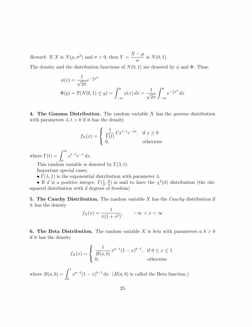
Remark. If X is N(µ, σ2) and σ > 0, then Y =X − µσ

is N(0, 1).

The density and the distribution functions of N(0, 1) are denoted by φ and Φ. Thus:

φ(x) =1√2πe−

12x2

Φ(y) = P(N(0, 1) ≤ y) =

∫ y

−∞φ(x) dx =

1√2π

∫ y

−∞e−

12x2 dx

4. The Gamma Distribution. The random variable X has the gamma distributionwith parameters λ, t > 0 if it has the density

fX(x) =

1

Γ(t)λtxt−1e−λx, if x ≥ 0

0, otherwise

where Γ(t) =

∫ ∞0

xt−1e−x dx.

This random variable is denoted by Γ(λ, t).Important special cases:• Γ(λ, 1) is the exponential distribution with parameter λ.• If d is a positive integer, Γ(1

2, d

2) is said to have the χ2(d) distribution (the chi-

squared distribution with d degrees of freedom)

5. The Cauchy Distribution. The random variable X has the Cauchy distribution ifit has the density

fX(x) =1

π(1 + x2), −∞ < x <∞

6. The Beta Distribution. The random variable X is beta with parameters a, b > 0if it has the density

fX(x) =

1

B(a, b)xa−1(1− x)b−1, if 0 ≤ x ≤ 1

0, otherwise

where B(a, b) =

∫ 1

0

xa−1(1− x)b−1 dx. (B(a, b) is called the Beta function.)

25

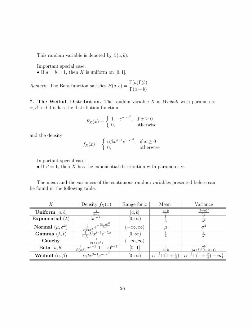
This random variable is denoted by β(a, b).

Important special case:• If a = b = 1, then X is uniform on [0, 1].

Remark: The Beta function satisfies B(a, b) =Γ(a)Γ(b)

Γ(a+ b).

7. The Weibull Distribution. The random variable X is Weibull with parametersα, β > 0 if it has the distribution function

FX(x) =

1− e−αxβ , if x ≥ 00, otherwise

and the density

fX(x) =

αβxβ−1e−αx

β, if x ≥ 0

0, otherwise

Important special case:• If β = 1, then X has the exponential distribution with parameter α.

The mean and the variances of the continuous random variables presented before canbe found in the following table:

X Density fX(x) Range for x Mean Variance

Uniform [a, b] 1b−a [a, b] a+b

2(b−a)2

12

Exponential (λ) λe−λx [0,∞) 1λ

1λ2

Normal (µ, σ2) 1√2πσ2

e−(x−µ)2

2σ2 (−∞,∞) µ σ2

Gamma (λ, t) 1Γ(t)

λtxt−1e−λx [0,∞) tλ

tλ2

Cauchy 1π(1+x2)

(−∞,∞) – –

Beta (a, b) 1B(a,b)

xa−1(1− x)b−1 [0, 1] aa+b

ab(a+b)2(a+b+1)

Weibull (α, β) αβxβ−1e−αxβ

[0,∞) α−1βΓ(1 + 1

β) α−

2βΓ(1 + 2

β)−m2

1

26

Note: In the last box, m1 denotes the mean of the Weibull distribution with parameters

α and β: m1 = α−1βΓ(1 + 1

β).

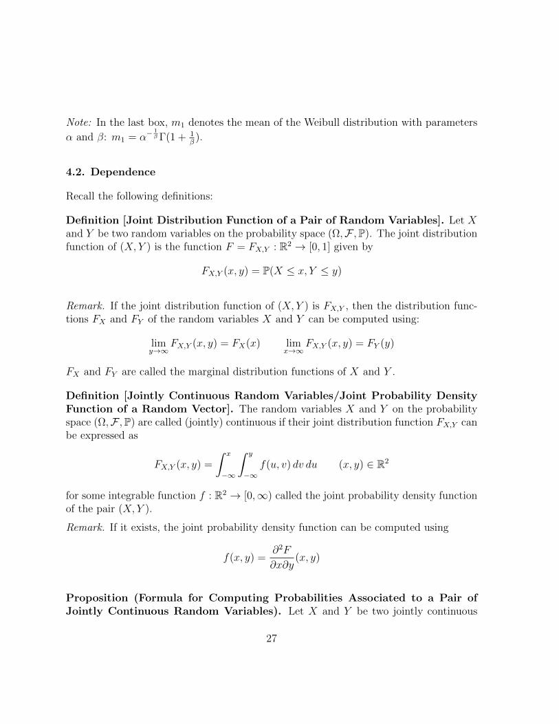
4.2. Dependence

Recall the following definitions:

Definition [Joint Distribution Function of a Pair of Random Variables]. Let Xand Y be two random variables on the probability space (Ω,F ,P). The joint distributionfunction of (X, Y ) is the function F = FX,Y : R2 → [0, 1] given by

FX,Y (x, y) = P(X ≤ x, Y ≤ y)

Remark. If the joint distribution function of (X, Y ) is FX,Y , then the distribution func-tions FX and FY of the random variables X and Y can be computed using:

limy→∞

FX,Y (x, y) = FX(x) limx→∞

FX,Y (x, y) = FY (y)

FX and FY are called the marginal distribution functions of X and Y .

Definition [Jointly Continuous Random Variables/Joint Probability DensityFunction of a Random Vector]. The random variables X and Y on the probabilityspace (Ω,F ,P) are called (jointly) continuous if their joint distribution function FX,Y canbe expressed as

FX,Y (x, y) =

∫ x

−∞

∫ y

−∞f(u, v) dv du (x, y) ∈ R2

for some integrable function f : R2 → [0,∞) called the joint probability density functionof the pair (X, Y ).

Remark. If it exists, the joint probability density function can be computed using

f(x, y) =∂2F

∂x∂y(x, y)

Proposition (Formula for Computing Probabilities Associated to a Pair ofJointly Continuous Random Variables). Let X and Y be two jointly continuous

27

random variables on the probability space (Ω,F ,P), with the joint probability densityfunction f = f(x, y). Suppose that B is a nice subset of R2. Then

P((X, Y ) ∈ B) =

∫ ∫B

f(x, y) dx dy

Remark. In particular, if B = [a, b]× [c, d], then

P(a ≤ X ≤ b, c ≤ Y ≤ d) = P((X, Y ) ∈ [a, b]× [c, d]) =

∫ d

c

∫ b

a

f(x, y) dx dy

Proposition (Formula for Computing the Marginal Density Functions). Let Xand Y be two jointly continuous random variables on the probability space (Ω,F ,P), withthe joint probability density function f = f(x, y). Then X and Y are continuous randomvariables and their density functions fX and fY can be computed using the formulas

fX(x) =

∫ ∞−∞

f(x, y) dy

fY (y) =

∫ ∞−∞

f(x, y) dx

The functions fX and fY are called the marginal probability density functions of Xand Y .

Proposition (Formula for Computing the Expectation of a Function of TwoJointly Continuous Random Variables). Let X and Y be two jointly continuousrandom variables on the probability space (Ω,F ,P), with the joint probability densityfunction f = f(x, y). Let g : R2 → R be a sufficiently nice function (Borel measurable).Then g(X, Y ) is a random variable whose expectation can be computed using

E(g(X, Y )) =

∫ ∞−∞

∫ ∞−∞

g(x, y)f(x, y) dx dy

Remark (Linearity). In particular, if a, b ∈ R and g(x, y) = ax+ by, we get E(g(X, Y )) =E(aX + bY ) = aE(X) + bE(Y ).

Definition (Independent Continuous Random Variables.) Let X and Y be twojointly continuous random variables on the probability space (Ω,F ,P), with joint distri-bution function F = F (x, y) and joint probability density function f = f(x, y). Suppose

28

that FX and FY are the marginal distribution functions of X and Y ; suppose also thatfX and fY are the marginal probability density functions of X and Y .

The random variables X and Y are independent if and only if

F (x, y) = FX(x)FY (y) for all x, y ∈ R

which is equivalent to

f(x, y) = fX(x) fY (y) for all x, y ∈ R

Theorem (Cauchy-Schwartz Inequality). For any pair X, Y of jointly continuousrandom variables, we have that

E(XY )2 ≤ E(X2)E(Y 2)

with equality if and only if there exist two constants a and b (not both 0) such thatP(aX = bY ) = 1.

Problem 1 [Buffon’s Needle]. A plane is ruled by the vertical lines x = n (n =0,±1,±2, . . .) and a needle of unit length is cast randomly on to the plane. What is theprobability that it intersects some line? (We suppose that the needle shows no preferencefor position or direction).

Problem 2 [Random Numbers]. Suppose that X, Y and Z are independent randomvariables uniformly distributed in [0, 1]. Compute the following probabilities:

a) P(Y ≤ 2X)

b) P(Y = 2X)

c) P(Z ≤ XY )

d) P(Z = XY )

Problem 3 [Buffon’s Needle Revisited]. Two grids of parallel lines are superimposed:the first grid contains lines distance a apart, and the second contains lines distance b apartwhich are perpendicular to those of the first set. A needle of length r (< mina, b) is

dropped at random. Show that the probability it intersects a line equals r(2a+2b−r)πab

.

Problem 4 [The Standard Bivariate Normal Distribution]. Let ρ be a constantsatisfying −1 < ρ < 1 and consider two jointly continuous random variables with thejoint density function f : R2 → R defined by

f(x, y) =1

2π√

1− ρ2exp

(− 1

2(1− ρ2)(x2 − 2ρxy + y2)

)29

(f is called the standard bivariate normal density of a pair of continuous random vari-ables)

a) Show that both X and Y are N(0, 1).

b) Show that cov(X, Y ) = ρ.

Problem 5. Suppose that X and Y are jointly continuous random variables with thejoint density function

f(x, y) =

1y

exp(−y − x

y

), if 0 < x, y <∞

0, otherwise

Show that the marginal density function of Y is the function fY (y) =

e−y, if y > 00, otherwise.

Table of discrete random variables:

X Values of X fX(k) Mean Variance

Bernoulli (p) 0,1 fX(0) = 1− p, fX(1) = p p p(1− p)Binomial (n, p) 0, 1, 2, . . . , n fX(k) =

(nk

)pk(1− p)n−k np np(1− p)

Poisson (λ) 0, 1, 2, . . . fX(k) = λk

k!e−λ λ λ

Geometric (p) 1, 2, . . . fX(k) = p(1− p)k−1 1p

1p2(1−p)

4.3. Conditional Distribution and Conditional Expectation

Definition [Conditional Distribution Function/Conditional Density Function].Suppose that X and Y are jointly continuous random variables with the joint density fX,Yand the marginal density functions fX and fY . Let x be a number such that fX(x) > 0.

The conditional distribution function of Y given X = x is the function FY |X(· |x)given by

FY |X(y |x) =

∫ y

−∞

fX,Y (x, v)

fX(x)dv

FY |X(y |x) is sometimes denoted by P(Y ≤ y |X = x).

The function fY |X(· |x) given by

fY |X(y |x) =fX,Y (x, y)

fX(x)

30

is called the conditional density function of FY |X .

Definition [Conditional Expectation]. Let X and Y be two jointly continuous ran-dom variables. The conditional expectation of Y given X is the random variable ψ(X),where the function ψ is defined on the set x, fX(x) > 0 by

ψ(x) = E(Y |X = x) =

∫ ∞−∞

y fY |X(y |x) dy

The random variable ψ(X) is denoted by E(Y |X).

Theorem (Law of Iterated Expectation). Let X and Y be two jointly continuousrandom variables and let ψ(X) = E(Y |X) be their conditional expectation. Then:

E(E(Y |X)) = E(Y )

4.4. Functions of Random Variables.

Theorem [The Change of Variables Formula in Two Dimensions]. Suppose thatT = T (x1, x2) = (y1(x1, x2), y2(x1, x2)) maps the domain A ⊆ R2 to the domain B ⊆ R2

and is invertible (one-to-one and onto). Suppose that the inverse of T is the functionT−1 : B → A, T−1(y1, y2) = (x1(y1, y2), x2(y1, y2)). Let g : A → R be an integrablefunction. We have∫ ∫

A

g(x1, x2) dx1dx2 =

∫ ∫B

g(x1(y1, y2), x2(y1, y2)) |J(y1, y2)| dy1dy2

where

J(y1, y2) =∂(x1, x2)

∂(y1, y2)=

∣∣∣∣∣ ∂x1∂y1

(y1, y2) ∂x1∂y2

(y1, y2)∂x2∂y1

(y1, y2) ∂x2∂y2

(y1, y2)

∣∣∣∣∣=∂x1

∂y1

(y1, y2)∂x2

∂y2

(y1, y2)− ∂x1

∂y2

(y1, y2)∂x2

∂y1

(y1, y2)

J(y1, y2) is called the Jacobian of the transformation T−1 at the point (y1, y2).

Theorem [The Change of the Joint Density Under a Function (in Two Dimen-sions)]. Suppose that the random variables X1 and X2 have the joint density functionfX1,X2 which is nonzero on the set A ⊆ R2 and zero outside the set A. Suppose that Bis a subset of R2 and T = T (x1, x2) : A→ B is invertible, with the inverse T−1 : B → A,

31

defined by T−1(y1, y2) = (x1(y1, y2), x2(y1, y2)). Let (Y1, Y2) = T (X1, X2). Then therandom variables Y1 and Y2 are jointly continuous and have the joint density

fY1,Y2(y1, y2) =

fX1,X2(x1(y1, y2), x2(y1, y2)) |J(y1, y2)|, if (y1, y2) ∈ B0, otherwise

where J(y1, y2) =∂(x1, x2)

∂(y1, y2)is the Jacobian of the transformation T−1 at (y1, y2).

4.5. Sums of Random Variables

Theorem [The Formula for the Density of the Sum of Two Jointly ContinuousRandom Variables]. Suppose that the random variables X and Y are jointly continu-ous and have the joint density function fX,Y . Then the random variable Z = X + Y iscontinuous and its density function fZ is given by the formula

fZ(z) =

∫ ∞−∞

fX,Y (x, z − x) dx

Definition [The Convolution of Two Functions]. The convolution of two functionsf : R→ R and g : R→ R is the function h = f ∗ g : R→ R defined by

h(z) = (f ∗ g) (z) =

∫ ∞−∞

f(x)g(z − x) dx

(assuming that the integral exists)

Remark: f ∗ g = g ∗ f , which is equivalent to

∫ ∞−∞

f(x)g(z−x) dx =

∫ ∞−∞

f(z−x)g(x) dx

for any z (assuming that the integrals exist).

Proposition [The Formula for the Density of the Sum of Two IndependentJointly Continuous Random Variables]. Suppose that the random variables X andY are jointly continuous, have the joint density function fX,Y and the marginal densitiesfX and fY . Suppose also that X and Y are independent. Then the random variableZ = X + Y is continuous and its density function fZ is given by the formula

fZ = fX ∗ fY

Remark: With the notations used before, we also have fZ = fY ∗ fX .

32

Problem 1. Let X and Y be independent N(0, 1) variables. Show that X+Y is N(0, 2).

Problem 2. Show that, if X is N(µ1, σ21) and Y is N(µ2, σ

22) and X and Y are indepen-

dent, then Z = X + Y is N(µ1 + µ2, σ21 + σ2

2).

4.6. Distributions Arising from the Normal Distribution

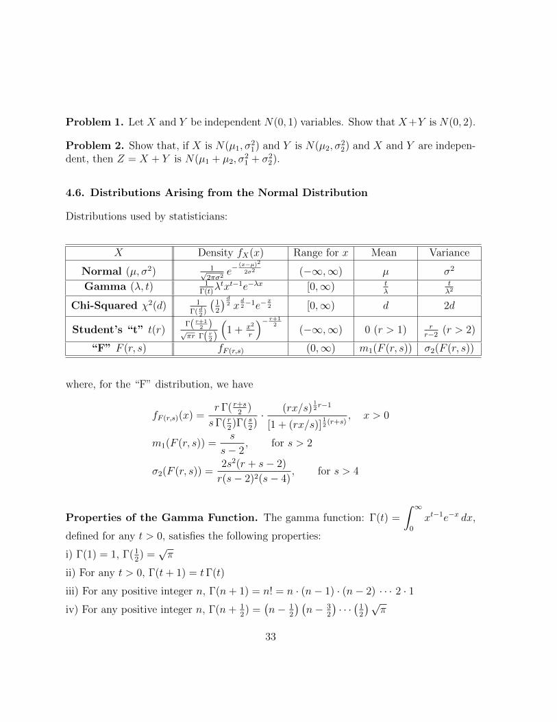
Distributions used by statisticians:

X Density fX(x) Range for x Mean Variance

Normal (µ, σ2) 1√2πσ2

e−(x−µ)2

2σ2 (−∞,∞) µ σ2

Gamma (λ, t) 1Γ(t)

λtxt−1e−λx [0,∞) tλ

tλ2

Chi-Squared χ2(d) 1Γ( d

2)

(12

) d2 x

d2−1e−

x2 [0,∞) d 2d

Student’s “t” t(r)Γ( r+1

2 )√πr Γ( r2)

(1 + x2

r

)− r+12

(−∞,∞) 0 (r > 1) rr−2

(r > 2)

“F” F (r, s) fF (r,s) (0,∞) m1(F (r, s)) σ2(F (r, s))

where, for the “F” distribution, we have

fF (r,s)(x) =r Γ( r+s

2)

sΓ( r2)Γ( s

2)· (rx/s)

12r−1

[1 + (rx/s)]12

(r+s), x > 0

m1(F (r, s)) =s

s− 2, for s > 2

σ2(F (r, s)) =2s2(r + s− 2)

r(s− 2)2(s− 4), for s > 4

Properties of the Gamma Function. The gamma function: Γ(t) =

∫ ∞0

xt−1e−x dx,

defined for any t > 0, satisfies the following properties:

i) Γ(1) = 1, Γ(12) =√π

ii) For any t > 0, Γ(t+ 1) = tΓ(t)

iii) For any positive integer n, Γ(n+ 1) = n! = n · (n− 1) · (n− 2) · · · 2 · 1iv) For any positive integer n, Γ(n+ 1

2) =

(n− 1

2

) (n− 3

2

)· · ·(

12

)√π

33

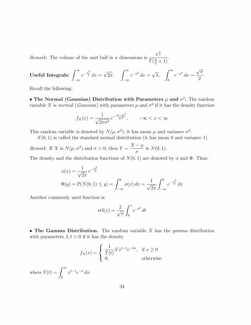
Remark: The volume of the unit ball in n dimensions isπn2

Γ(n2

+ 1).

Useful Integrals:

∫ ∞−∞

e−x2

2 dx =√

2π,

∫ ∞−∞

e−x2

dx =√π,

∫ ∞0

e−x2

dx =

√π

2.

Recall the following:

• The Normal (Gaussian) Distribution with Parameters µ and σ2. The randomvariable X is normal (Gaussian) with parameters µ and σ2 if it has the density function

fX(x) =1√

2πσ2e−

(x−µ)2

2σ2 , −∞ < x <∞

This random variable is denoted by N(µ, σ2); it has mean µ and variance σ2.N(0, 1) is called the standard normal distribution (it has mean 0 and variance 1).

Remark. If X is N(µ, σ2) and σ > 0, then Y =X − µσ

is N(0, 1).

The density and the distribution functions of N(0, 1) are denoted by φ and Φ. Thus:

φ(x) =1√2π

e−x2

2

Φ(y) = P(N(0, 1) ≤ y) =

∫ y

−∞φ(x) dx =

1√2π

∫ y

−∞e−

x2

2 dx

Another commonly used function is

erf(x) =2√π

∫ x

0

e−t2

dt

• The Gamma Distribution. The random variable X has the gamma distributionwith parameters λ, t > 0 if it has the density

fX(x) =

1

Γ(t)λtxt−1e−λx, if x ≥ 0

0, otherwise

where Γ(t) =

∫ ∞0

xt−1e−x dx.

34

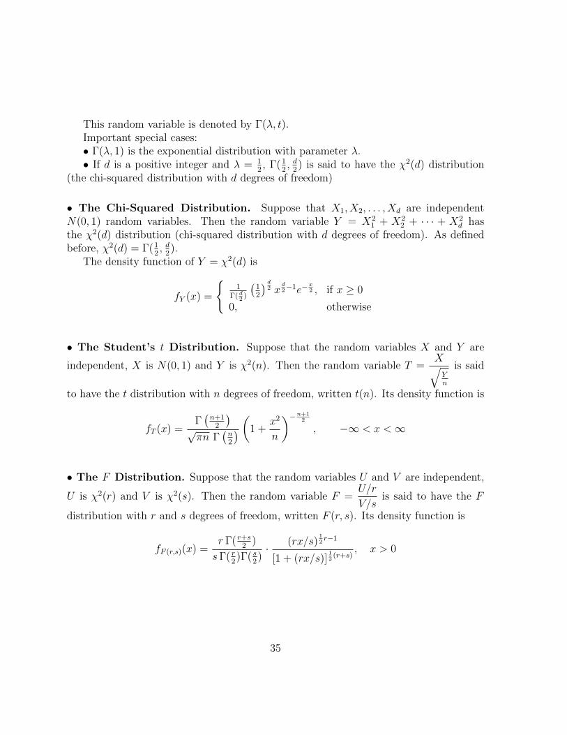
This random variable is denoted by Γ(λ, t).Important special cases:• Γ(λ, 1) is the exponential distribution with parameter λ.• If d is a positive integer and λ = 1

2, Γ(1

2, d

2) is said to have the χ2(d) distribution

(the chi-squared distribution with d degrees of freedom)

• The Chi-Squared Distribution. Suppose that X1, X2, . . . , Xd are independentN(0, 1) random variables. Then the random variable Y = X2

1 + X22 + · · · + X2

d hasthe χ2(d) distribution (chi-squared distribution with d degrees of freedom). As definedbefore, χ2(d) = Γ(1

2, d

2).

The density function of Y = χ2(d) is

fY (x) =

1

Γ( d2

)

(12

) d2 x

d2−1e−

x2 , if x ≥ 0

0, otherwise

• The Student’s t Distribution. Suppose that the random variables X and Y are

independent, X is N(0, 1) and Y is χ2(n). Then the random variable T =X√Yn

is said

to have the t distribution with n degrees of freedom, written t(n). Its density function is

fT (x) =Γ(n+1

2

)√πn Γ

(n2

) (1 +x2

n

)−n+12

, −∞ < x <∞

• The F Distribution. Suppose that the random variables U and V are independent,

U is χ2(r) and V is χ2(s). Then the random variable F =U/r

V/sis said to have the F

distribution with r and s degrees of freedom, written F (r, s). Its density function is

fF (r,s)(x) =r Γ( r+s

2)

sΓ( r2)Γ( s

2)· (rx/s)

12r−1

[1 + (rx/s)]12

(r+s), x > 0

35

FINDING CONFIDENCE INTERVALS

Definition [Sample Mean]. The sample mean of a set of random variablesX1, X2, . . . , Xn

is the random variable

X =

∑nk=1Xk

n

Definition [Sample Variance]. The sample variance of a set of random variablesX1, X2, . . . , Xn is the random variable S2 defined by

S2 =

∑nk=1(Xk −X)2

n− 1

where X is the sample mean.

Remark: If X1, X2, . . . , Xn are independent N(µ, σ2) random variables, X is their samplemean, and S2 is their sample variance, then E(X) = µ and E(S2) = σ2.

Theorem [The Distributions of X and S2]. If X1, X2, . . . , Xn are independentN(µ, σ2) random variables, X is their sample mean, and S2 is their sample variance,then:a) X is N(µ, σ

2

n)

b) n−1σ2 S

2 is χ2(n− 1).

Remark: X is N(µ, σ2

n) implies that

√n(X−µ)σ

is N(0, 1).

Theorem [Confidence Interval for the Mean of a Population]. If X1, X2, . . . , Xn

are independent N(µ, σ2) random variables, X is their sample mean, and S2 is theirsample variance, then:

a)√n(X−µ)S

is t(n− 1)

b) If 0 < α < 1 and t∗ is chosen such that P(−t∗ ≤ t(n − 1) ≤ t∗) = 1 − α, then

P(X − t∗S√

n≤ µ ≤ X + t∗S√

n

)= 1 − α. This means that

[X − t∗S√

n, X + t∗S√

n

]is a (1 − α)

confidence interval for µ.

4.7. Sampling From a Distribution

We describe two methods of sampling from a distribution: 1. The inverse transformtechnique and 2. The rejection method.

36

Sampling From a Distribution Using the Inverse Transform Technique. Sup-pose that the function F : R→ [0, 1] is the distribution function of the random variableY and let U be a random variable uniformly distributed in [0, 1]. Then:

a) If F is a continuous function, the random variable X = F−1(U) has the distributionfunction F (hence the same distribution as Y ).

b) If Y is discrete with values in 0, 1, 2, . . ., then the random variable X defined by

X = k if and only if F (k − 1) < U ≤ F (k)

has the distribution F (hence the same distribution as Y)

Sampling From a Distribution Using the Rejection Method. We want to samplefrom a distribution having the density function f .

Suppose that the pair (U,Z) of random variables satisfies the following properties:i) U and Z are independentii) U is uniformly distributed on [0, 1]iii) Z has the density function fZ and there exists a constant a ∈ R such that f(z) ≤

afZ(z) for all z.

Then P(Z ≤ x | aUfZ(Z) ≤ f(Z)) =

∫ x

−∞f(z) dz, which means that, conditional

on the event E = aUfZ(Z) ≤ f(Z), the random variable Z has the required densityfunction f .

How we use this:Step 1. Use a random number generator to obtain a pair (U,Z) as above.Step 2. Check whether the event E occurs. If E occurs, keep Z. If E doesn’t occur,

reject the pair (U,Z) and go back to Step 1.

Problem 1. Let X and Y be independent N(0, 1) variables. Show that X2 + Y 2 isχ2(2).

Problem 2 [Binomial Sampling]. Let U1, U2, . . . , Un, . . . be independent random vari-ables with the uniform distribution on [0, 1]. The sequence Xk = IUk≤p of indicatorvariables contains independent random variables having the Bernoulli distribution withparameter p. The sum S =

∑nk=1Xk has the bin(n, p) distribution.

Problem 3 [Gamma Sampling]. Let U1, U2, . . . , Un, . . . be independent random vari-ables with the uniform distribution on [0, 1]. The sequence Xk = − 1

λln(1−Uk) contains

37

independent random variables having the exponential distribution with parameter λ. Thesum S =

∑nk=1 Xk has the Γ(λ, n) distribution.

Theorem [Confidence Interval for the Mean of a Population]. If X1, X2, . . . , Xn

are independent N(µ, σ2) random variables, X is their sample mean, and S2 is theirsample variance, then:

a)√n(X−µ)S

is t(n− 1)

b) If 0 < α < 1 and t∗ is chosen such that P(−t∗ ≤ t(n − 1) ≤ t∗) = 1 − α, then

P(X − t∗S√

n≤ µ ≤ X + t∗S√

n

)= 1 − α. This means that

[X − t∗S√

n, X + t∗S√

n

]is a (1 − α)

confidence interval for µ.

Chapter 5 - The Law of Large Numbers and the Central Limit Theorem

5.1. Characteristic Functions.

Definition [The Moment Generating Function of a Random Variable]. LetX : Ω → R be a random variable on the probability space (Ω,F ,P). The momentgenerating function of X is the function MX : R→ [0,∞) given by MX(t) = E(etX).

Remark: There exist random variables X and real numbers t for which E(etX) is notdefined (hence the moment generating function of X is not defined at t).

Proposition [Properties of the Moment Generating Function of a RandomVariable]. If X is a random variable for which all the moments E(Xk) exist and MX isits moment generating function then:

a) MX(0) = 1

b) MX(t) =∞∑k=0

E(Xk)

k!tk

c) For any positive integer k, we have E(Xk) = M (k)(0)

d) If X and Y are independent, MX+Y (t) = MX(t)MY (t)

Complex Numbers - Basic Properties. For any (a, b) ∈ R2 we consider the expres-sion a+bi. Let C = the set of all numbers of the form z = a+bi, a, b ∈ R. C is calledthe set of complex numbers. The number i is not real and has the property i2 = −1.

38

• Sum of complex numbers. (a+ bi) + (c+ di) = (a+ c) + (b+ d)i

• Product of complex numbers. (a+ bi)(c+ di) = (ac− bd) + (ad+ bc)i

• The absolute value of a complex number. If z = a+bi, with a, b ∈ R, then |z| =√a2 + b2

• The conjugate of a complex number. If z = a+ bi, with a, b ∈ R, then z = a− bi. Animmediate computation shows that zz = |z|2

• The exponential function. If α ∈ R, then we define eiα = cosα + i sinα. It is nothard to see that ei(α+β) = eiαeiβ for any α, β ∈ R. For any z = a + ib, we defineea+ib = eaeib = ea(cos b+ i sin b).

For any a, b ∈ R, we have |ea+bi| = ea. In particular, for any b ∈ R, |eib| = 1. Also,for any a, b ∈ R, ea+bi = ea−bi. In particular, for any b ∈ R, ebi = e−bi.

Definition [The Characteristic Function of a Random Variable]. Let X : Ω→ Rbe a random variable on the probability space (Ω,F ,P). The characteristic function ofX is the function φX : R→ C given by φX(t) = E(eitX).

Remark: φX(t) = E(eitX) = E(cos(tX)) + iE(sin(tX)).

Proposition [Properties of the Characteristic Function of a Random Vari-able]. If X is a random variable for which all the moments E(Xk) exist and φX is itscharacteristic function then:

a) φX(0) = 1

b) |φX(t)| ≤ 1 for all t ∈ Rc) φX is (uniformly) continuous

d) For any positive integer n, any real numbers t1, t2, . . . , tn, and any complex numbers

z1, z2, . . . , zn, we haven∑

j,k=1

φX(tj − tk)zj zk ≥ 0

e) φX(t) =∞∑k=0

E(Xk)

k!(it)k

f) For any positive integer k, we have E(Xk) =φ(k)(0)

ik

Theorem [The Characteristic Function of a Sum of Two Independent RandomVariables]. If X and Y are independent random variables, then φX+Y (t) = φX(t)φY (t).

39

Theorem [The Characteristic Function of a Linear Function of a RandomVariable]. If X is a random variable, a, b ∈ R and Y = aX+ b, then φY (t) = eitbφX(at).

Definition [The Joint Characteristic Function of Two Random Variables]. LetX and Y be two random variables. The joint characteristic function of X and Y is thefunction φX,Y : R2 → R given by φX,Y (s, t) = E(eisXeitY ).

Remark. φX,Y (s, t) = φsX+tY (1).

Theorem. Let X and Y be two random variables with characteristic functions φX andφY . Suppose that φX,Y is the joint characteristic function of X and Y . Then X and Yare independent if and only if φX,Y (s, t) = φX(s)φY (t) for all s, t ∈ R.

5.2. Examples of Characteristic Functions.

1. The Bernoulli Distribution. If X = Bernoulli(p), where 0 < p < 1, then φX(t) =1− p+ peit.

2. The Binomial Distribution. If X = bin(n, p), where 0 < p < 1 and n is a positiveinteger, then φX(t) = (1− p+ peit)n.

3. The Exponential Distribution. If X = Exponential(λ), where λ > 0, then

φX(t) =λ

λ− it.

4. The Cauchy Distribution. If X has the Cauchy distribution, then φX(t) = e−|t|.

5. The Normal Distribution. If X has the N(µ, σ2) distribution, then φX(t) =

eiµt−12σ2t2 .

6. The Gamma Distribution. If X has the Γ(λ, s) distribution, then φX(t) =(λ

λ− it

)s. In particular, if X has the χ2(d) distribution (which is Γ(1

2, d

2)), then

φX(t) = (1− 2it)−d2 .

X Values of X fX(k) φX(t) MX(t)

Bernoulli (p) 0,1 fX(0) = 1− p, fX(1) = p 1− p+ peit 1− p+ pet

Binomial (n, p) 0, 1, 2, . . . , n fX(k) =(nk

)pk(1− p)n−k (1− p+ peit)n (1− p+ pet)n

Poisson (λ) 0, 1, 2, . . . fX(k) = λk

k!e−λ eλ(eit−1) eλ(et−1)

Geometric (p) 1, 2, . . . fX(k) = p(1− p)k−1 peit

1−(1−p)eitpet

1−(1−p)et

40

X Density fX(x) Range for x φX(t) MX(t)

Uniform [a, b] 1b−a [a, b] eitb−eita

it(b−a)etb−etat(b−a)

Exponential (λ) λe−λx [0,∞) λλ−it

λλ−t

Normal (µ, σ2) 1√2πσ2

e−(x−µ)2

2σ2 (−∞,∞) eiµt−12σ2t2 eµt+

12σ2t2

Gamma (λ, s) 1Γ(s)

λsxs−1e−λx [0,∞)(

λλ−it

)s (λλ−t

)sCauchy 1

π(1+x2)(−∞,∞) e−|t| –

5.3. Inversion and Continuity Theorems.

Theorem [Inversion Theorem 1: Recovering the Density Function from theCharacteristic Function]. Suppose that X is a continuous random variable with thedensity function fX and the characteristic function φX . Then

fX(x) =1

2π

∫ ∞−∞

e−itxφ(t) dt

at every point x at which f is differentiable.

Theorem [Inversion Theorem 2: Recovering the Distribution Function fromthe Characteristic Function]. Suppose that the random variable X has distributionfunction FX and the characteristic function φX . We define the function FX : R→ [0, 1]by

FX(x) =1

2

FX(x) + lim

y↑xFX(y)

Then

F (b)− F (a) = limN→∞

∫ N

−N

e−iat − e−ibt

2πitφ(t) dt

Theorem [A Random Variable is Uniquely Determined by Its CharacteristicFunction]. The random variables X and Y have the same characteristic function if andonly if they have the same distribution function.

Definition [Convergence of Distribution Functions]. We say that the sequence ofdistributions F1, F2, . . . converges to the distribution function F , (and we write Fn → F ),if F (x) = limn→∞ Fn(x) at each point where F is continuous.

Theorem [The Continuity Theorem]. Let X1, X2, . . . be random variables with thedistribution functions F1, F2, . . . and the characteristic functions φ1, φ2, . . ..

41

a) If there exists a random variable X with distribution F and characteristic function φsuch that Fn → F , then φn(t)→ φ(t) for any t ∈ R.

b) If limn→∞ φn(t) = φ(t) for any t and the limit function φ(t) is continuous at t = 0,then φ is the characteristic function of a random variable X. Furthermore, Fn → F ,where F is the distribution function of X.

Problem 1. If X is N(0, 1), show that its moment generating function is MX(s) = es2

2

and its characteristic function is φX(t) = e−t2

2 .

Problem 2. If Y is N(µ, σ2), show that its characteristic function is φY (t) = eiµt−12σ2t2 .

5.4. Two Limit Theorems

Definition [Convergence in Distribution]. Let X,X1, X2, . . . be a sequence of ran-dom variables with the distribution functions F, F1, F2, . . .. We say that Xn converges in

distribution to X (and we write XnD−−→ X) as n→∞ if Fn → F as n→∞.

Remark. The Continuity Theorem from the previous section shows that if X,X1, X2, . . . isa sequence of random variables with distribution functions F, F1, F2, . . . and characteristic

functions φ, φ1, φ2, . . ., then, in order to prove that XnD−−→ X, it suffices to show that

limn→∞ φn(t) = φ(t) for any t and φ(t) is continuous at t = 0.

A useful limit: If limn→∞ f(n) = 0 and limn→∞ g(n) =∞, then

limn→∞

(1 + f(n))g(n) = eL where L = limn→∞

[f(n)g(n)]

(assuming that all the limits exist)

Theorem [The Law of Large Numbers]. Let X1, X2, . . . be a sequence of independentidentically distributed random variables with finite mean µ. For any n, we define Sn =X1 +X2 + · · ·+Xn. Then

1

nSn

D−−→ µ as n→∞

Theorem [The Central Limit Theorem]. Let X1, X2, . . . be a sequence of inde-pendent identically distributed random variables with finite mean µ and finite non-zerovariance σ2. For any n, we define Sn = X1 +X2 + · · ·+Xn. Then

Sn − nµ√nσ2

D−−→ N(0, 1) as n→∞

42