Pathways and Energy Landscapes
55
Pathways and Energy Landscapes by Semen Trygubenko (sat39|at|cam.ac.uk)
Transcript of Pathways and Energy Landscapes

Pathways and Energy Landscapesby Semen Trygubenko (sat39|at|cam.ac.uk)

Acknowledgements
Dr David J. Wales
Darwin CollegeCambridge Overseas Trust
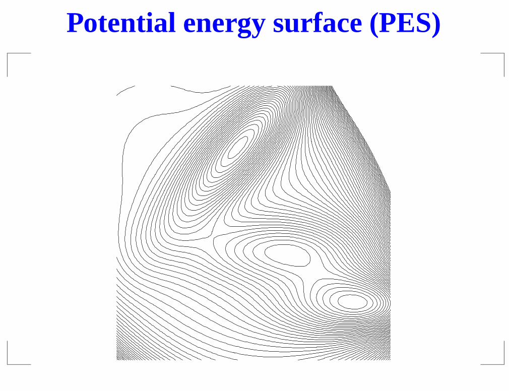
Potential energy surface (PES)
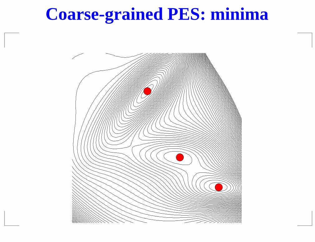
Coarse-grained PES: minima
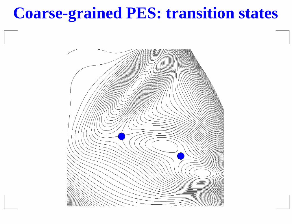
Coarse-grained PES: transition states
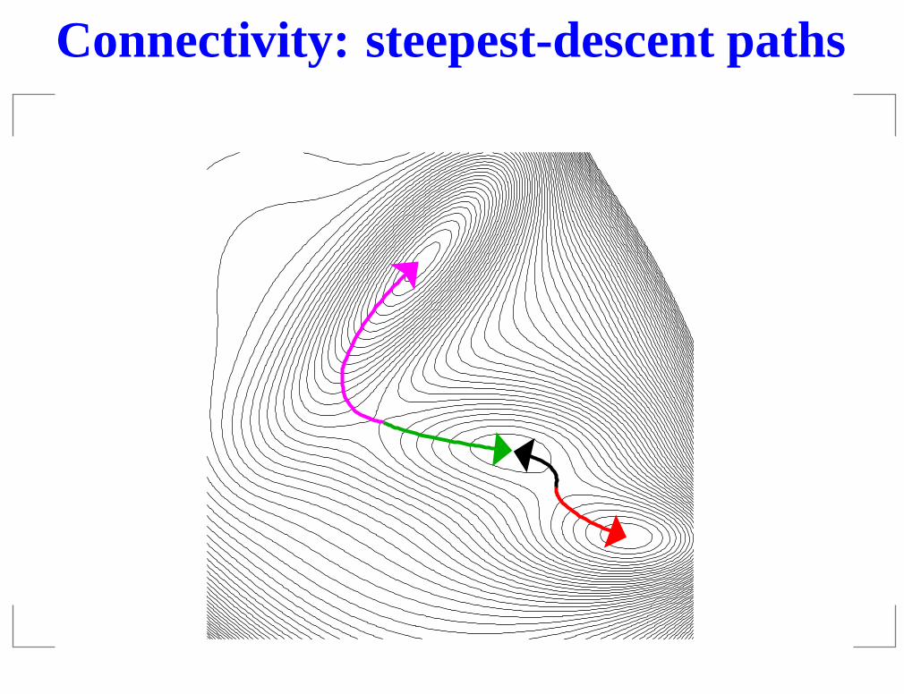
Connectivity: steepest-descent paths
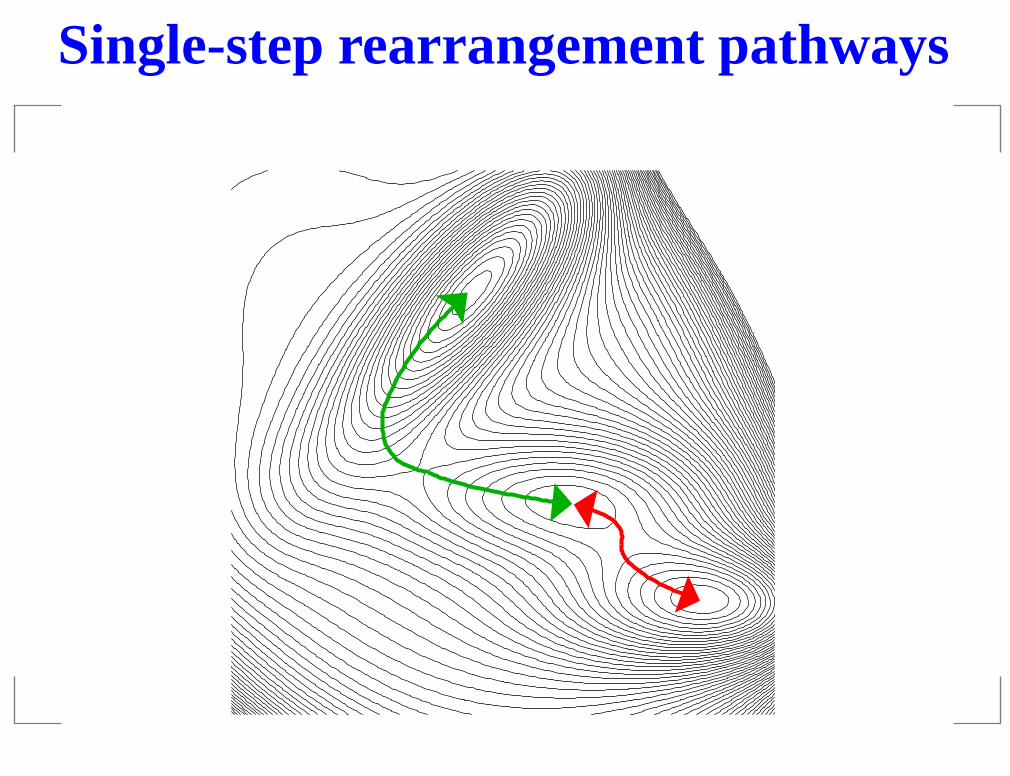
Single-step rearrangement pathways
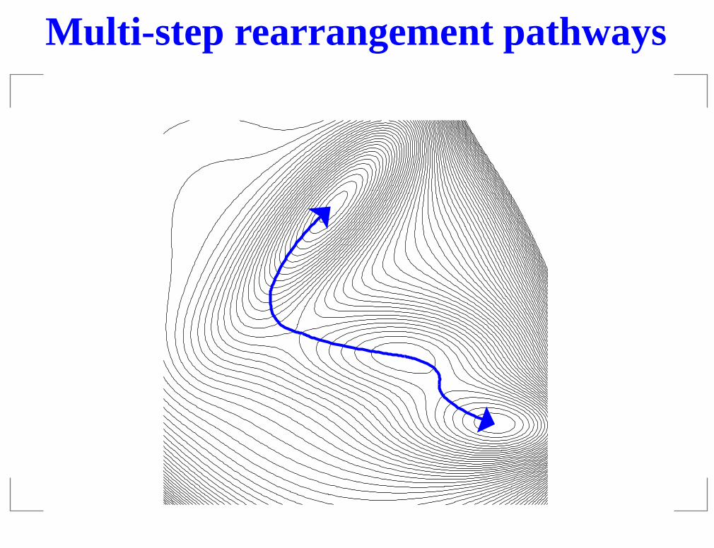
Multi-step rearrangement pathways
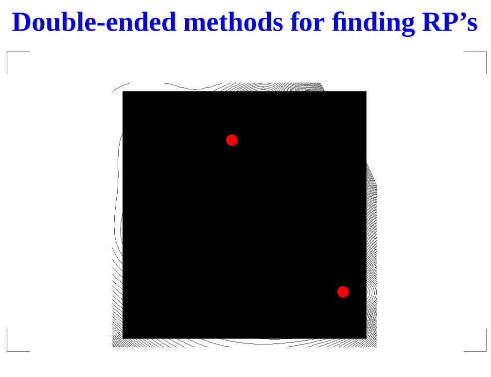
Double-ended methods for finding RP’s
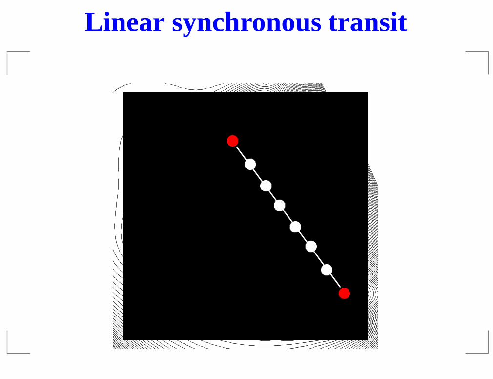
Linear synchronous transit
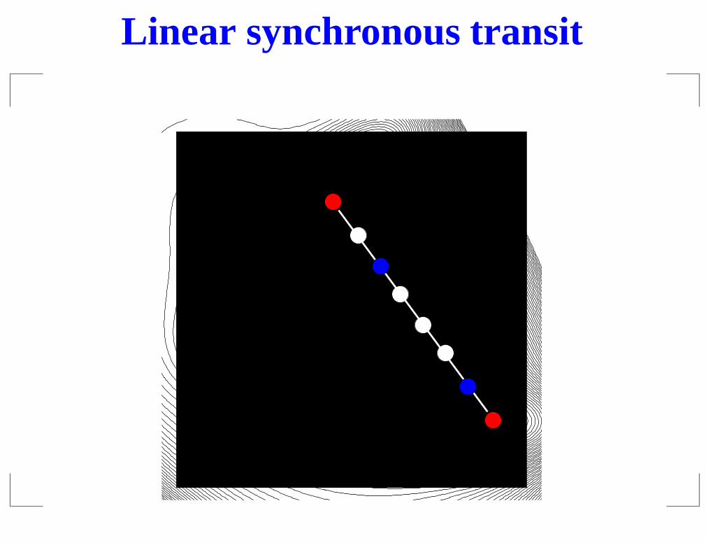
Linear synchronous transit
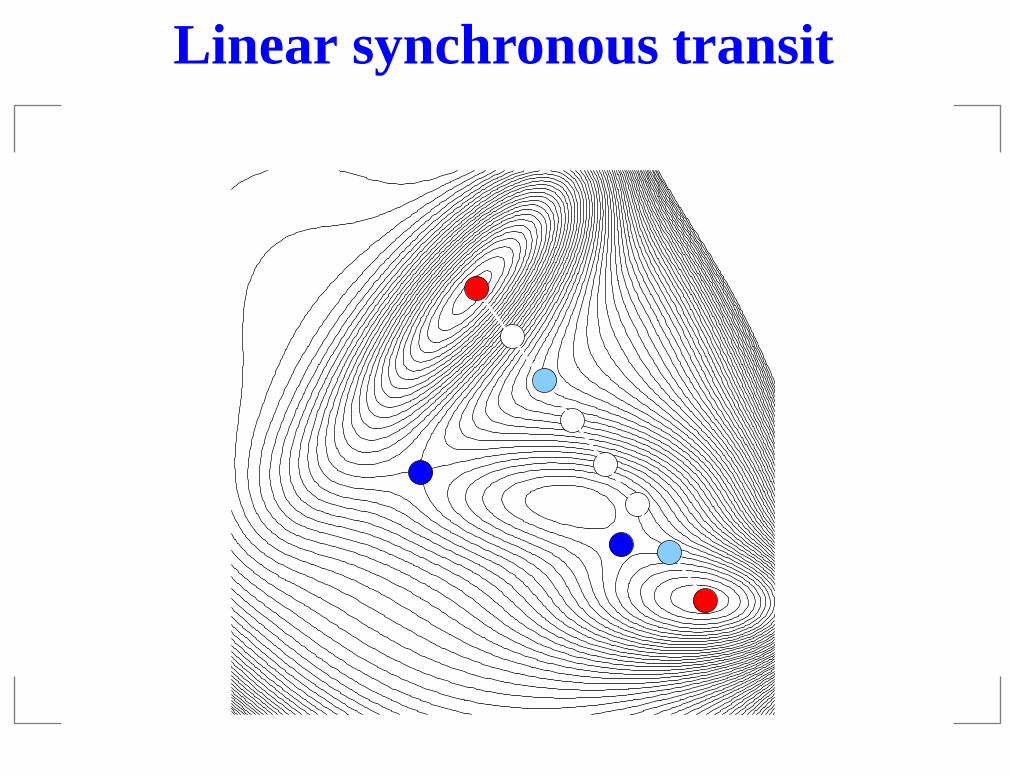
Linear synchronous transit
g + g
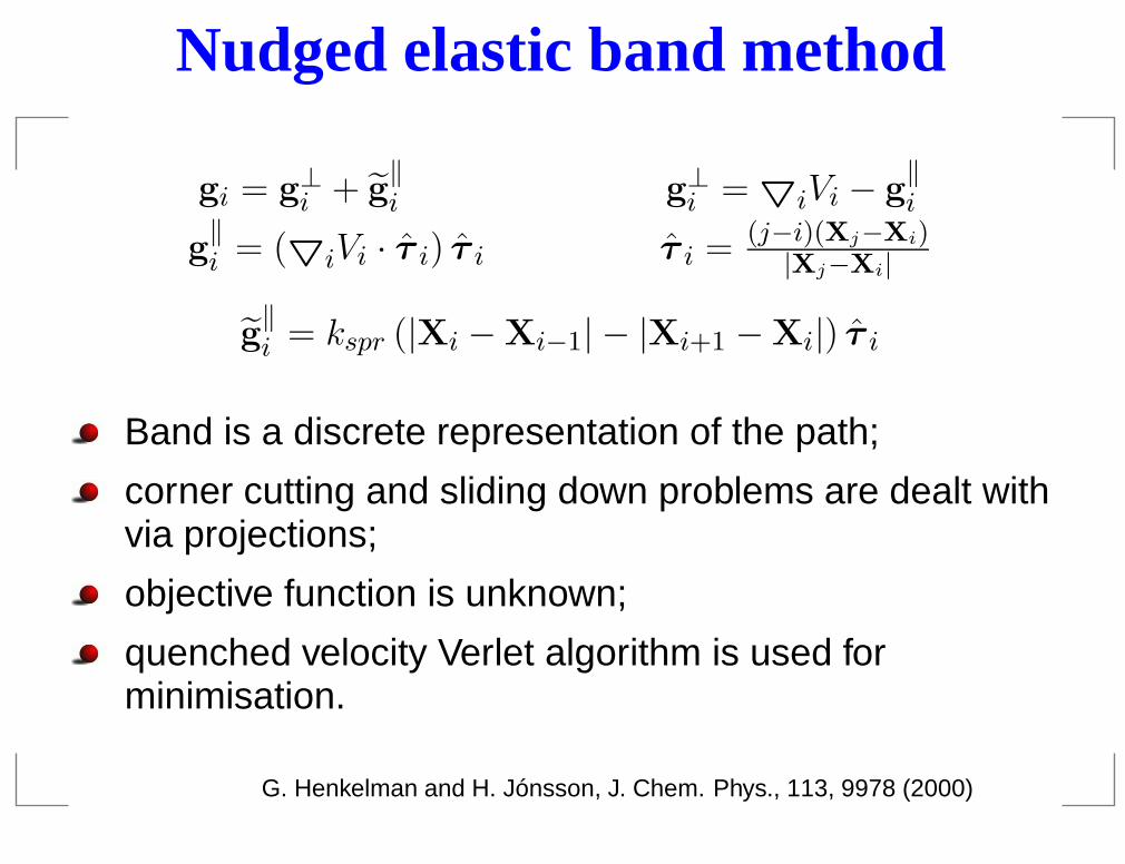
Nudged elastic band method
gi = g⊥i + g‖i g⊥i = 5iVi − g
‖i
g‖i = (5iVi · τ i) τ i τ i = (j−i)(Xj−Xi)
|Xj−Xi|
g‖i = kspr (|Xi − Xi−1| − |Xi+1 −Xi|) τ i
Band is a discrete representation of the path;
corner cutting and sliding down problems are dealt withvia projections;
objective function is unknown;
quenched velocity Verlet algorithm is used forminimisation.
G. Henkelman and H. Jónsson, J. Chem. Phys., 113, 9978 (2000)
g‖ + g⊥ (g‖ and g⊥ are projected out)
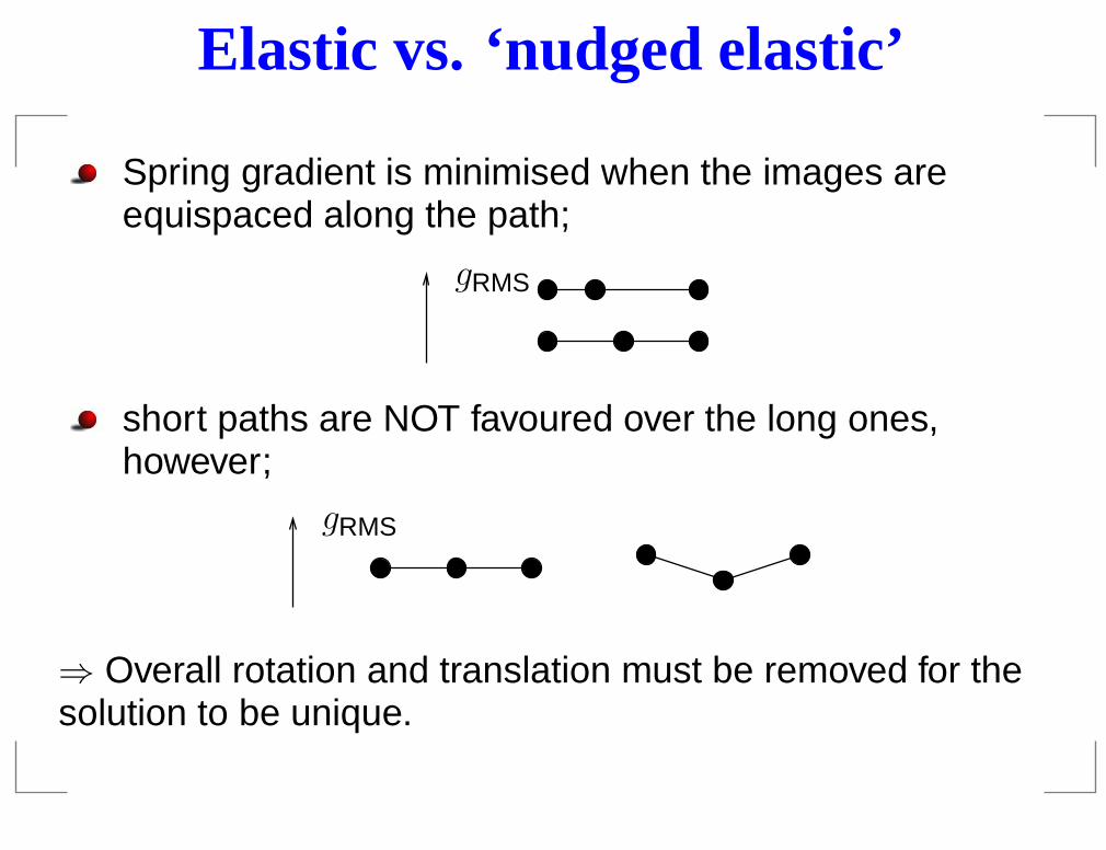
Elastic vs. ‘nudged elastic’
Spring gradient is minimised when the images areequispaced along the path;
PSfrag replacements gRMS
short paths are NOT favoured over the long ones,however;
PSfrag replacements gRMS
⇒ Overall rotation and translation must be removed for thesolution to be unique.

NEB highlights
Band is a discrete representation of a pathway;
Initial guess is required;
Two parameters must be provided:number of images;spring force constant;
Minimisation can easily become ill-conditioned;
Object function is unknown;
Problems with convergence and termination criteria;
ORT removal affects:stability;efficiency.
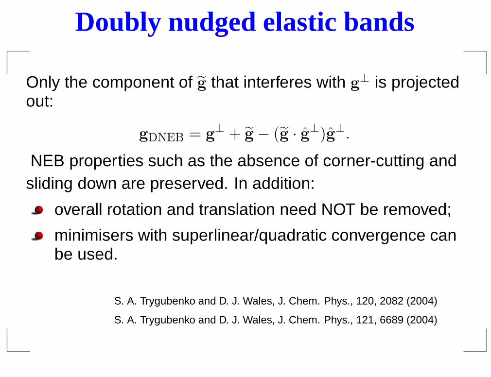
Doubly nudged elastic bands
Only the component of g that interferes with g⊥ is projectedout:
gDNEB = g⊥ + g − (g · g⊥)g⊥.
NEB properties such as the absence of corner-cutting andsliding down are preserved. In addition:
overall rotation and translation need NOT be removed;
minimisers with superlinear/quadratic convergence canbe used.
S. A. Trygubenko and D. J. Wales, J. Chem. Phys., 120, 2082 (2004)
S. A. Trygubenko and D. J. Wales, J. Chem. Phys., 121, 6689 (2004)
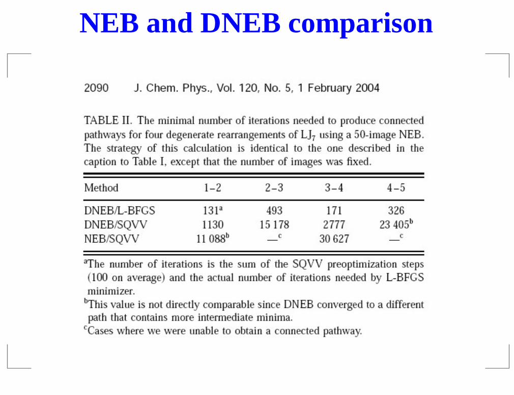
NEB and DNEB comparison

Summary 1
What is a RP?single-step and multi-step paths;a discrete representation.
How to find a RP?double-ended methods;nudged elastic bands;doubly nudged elastic bands.
Why pathways are important?Mechanism;Kinetics.
Properties of RP.
Why some RP are difficult to find?
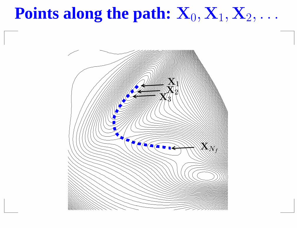
Points along the path: X0,X1,X2, . . .
PSfrag replacements
X1X2
X3
XNf
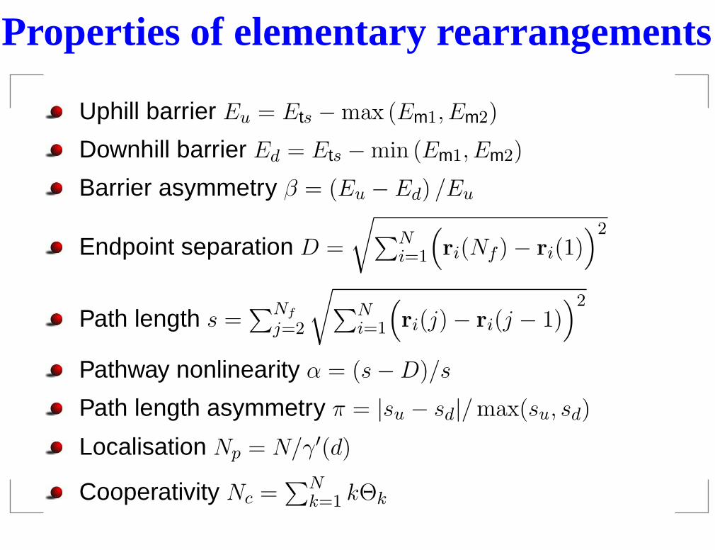
Properties of elementary rearrangements
Uphill barrier Eu = Ets − max (Em1, Em2)
Downhill barrier Ed = Ets − min (Em1, Em2)
Barrier asymmetry β = (Eu − Ed) /Eu
Endpoint separation D =
√∑N
i=1
(ri(Nf ) − ri(1)
)2
Path length s =∑Nf
j=2
√∑N
i=1
(ri(j) − ri(j − 1)
)2
Pathway nonlinearity α = (s − D)/s
Path length asymmetry π = |su − sd|/max(su, sd)
Localisation Np = N/γ′(d)
Cooperativity Nc =∑N
k=1 kΘk
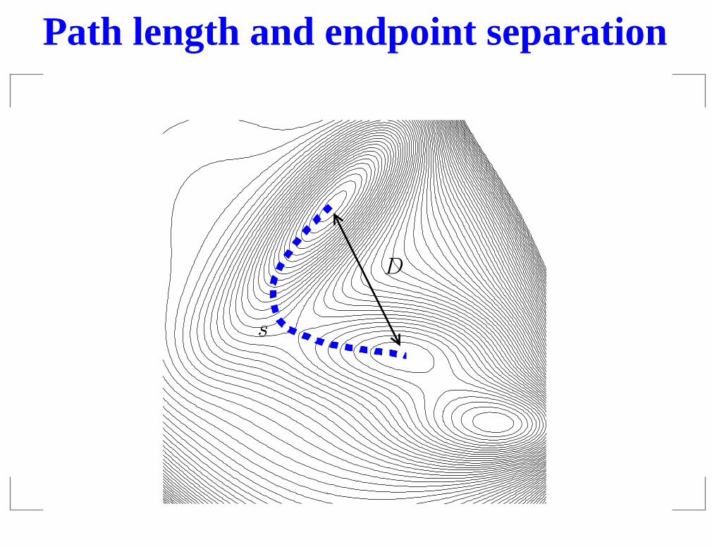
Path length and endpoint separation
PSfrag replacements
D
s
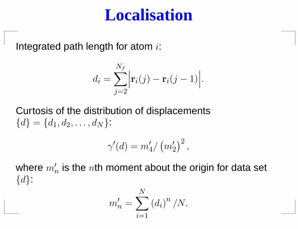
Localisation
Integrated path length for atom i:
di =
Nf∑
j=2
∣∣∣ri(j) − ri(j − 1)∣∣∣.
Curtosis of the distribution of displacements{d} = {d1, d2, . . . , dN}:
γ′(d) = m′4/(m′2
)2,
where m′n is the nth moment about the origin for data set{d}:
m′n =N∑
i=1
(di)n /N.
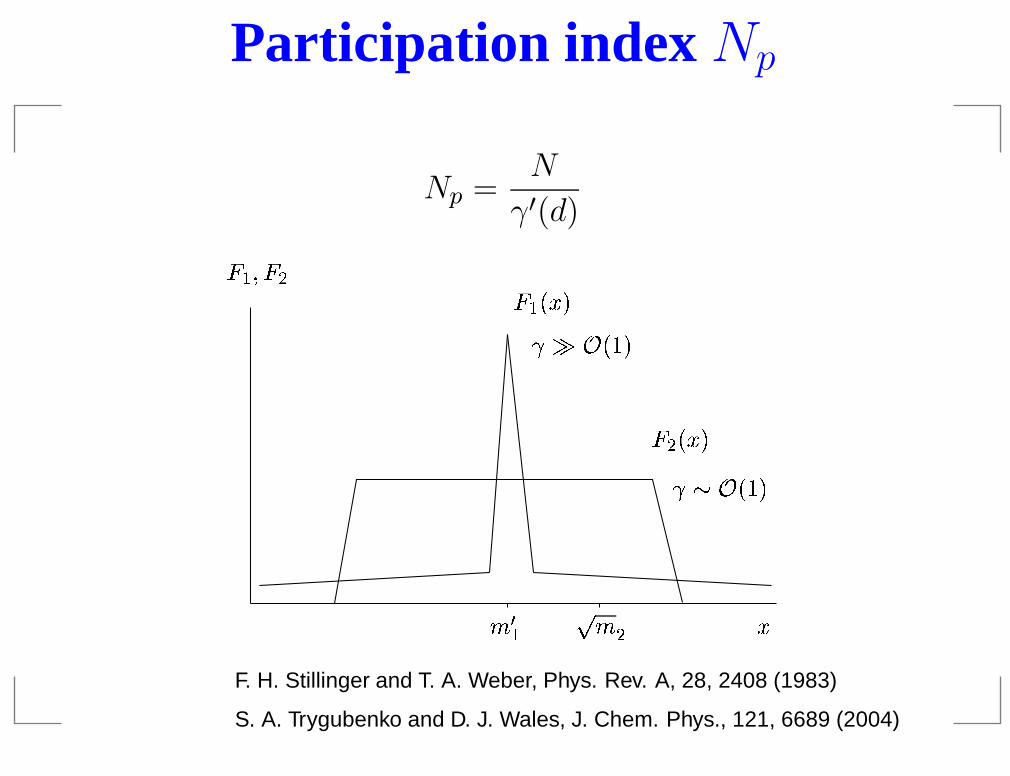
Participation index Np
Np =N
γ′(d)
�����
���
��� ���
��� � � � � �
� � �
� ��
� � � �
F. H. Stillinger and T. A. Weber, Phys. Rev. A, 28, 2408 (1983)
S. A. Trygubenko and D. J. Wales, J. Chem. Phys., 121, 6689 (2004)
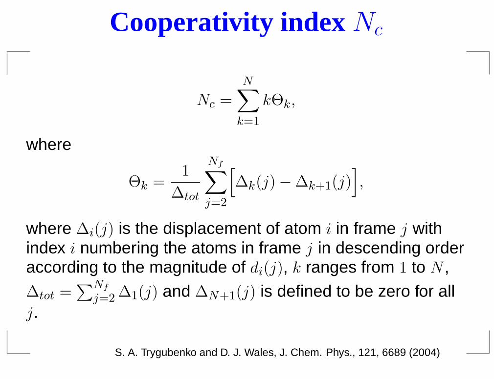
Cooperativity index Nc
Nc =N∑
k=1
kΘk,
where
Θk =1
∆tot
Nf∑
j=2
[∆k(j) − ∆k+1(j)
],
where ∆i(j) is the displacement of atom i in frame j withindex i numbering the atoms in frame j in descending orderaccording to the magnitude of di(j), k ranges from 1 to N ,
∆tot =∑Nf
j=2 ∆1(j) and ∆N+1(j) is defined to be zero for allj.
S. A. Trygubenko and D. J. Wales, J. Chem. Phys., 121, 6689 (2004)
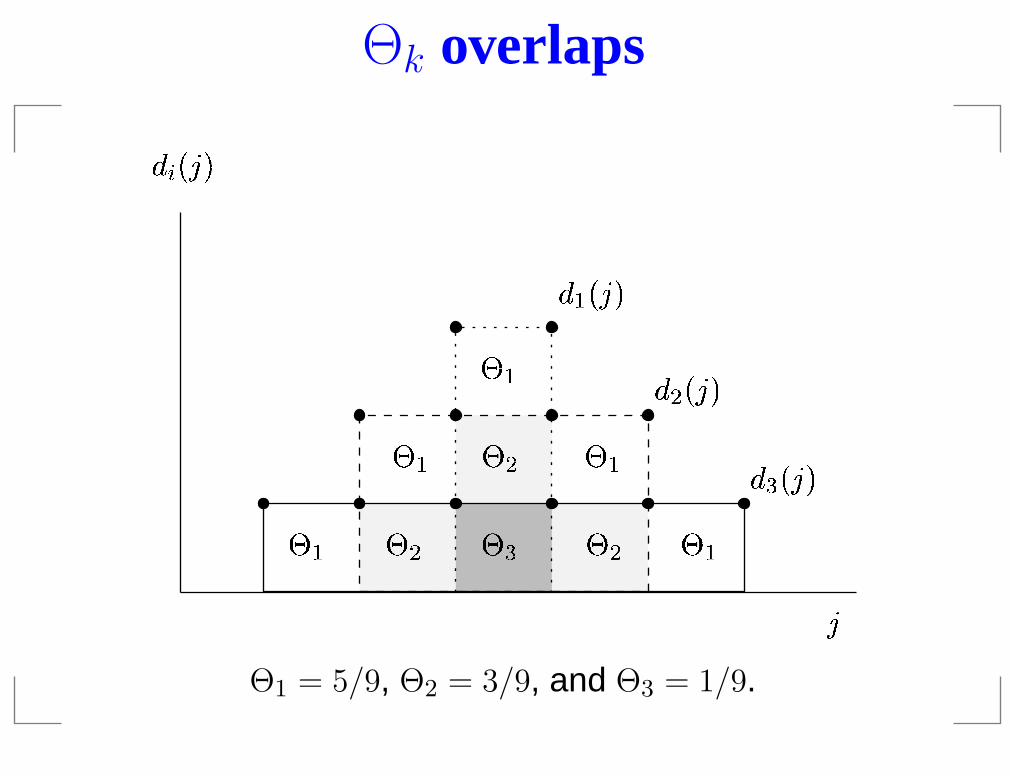
Θk overlaps
��� �� �
�
��� �� �
�� �� �
�� �� �
� �� �
� � � �
� �
� � � �
� ��
Θ1 = 5/9, Θ2 = 3/9, and Θ3 = 1/9.
Examples of usage
Np ∈ [1, N ] (usually)Nc ∈ [1, N ]Nc 6 Np.


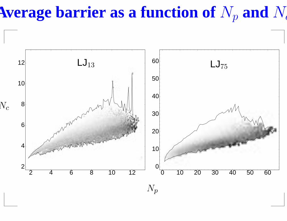
Average barrier as a function of Np and NcPSfrag replacements
Np
Nc
60
60
50
50
40
40
30
30
20
20
12
12
10
10
10
10
8
8
6
6
4
42
20
0
LJ13 LJ75
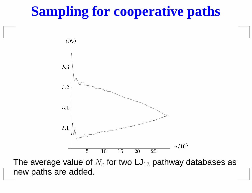
Sampling for cooperative paths
� � � � � � � � �
���
����
����
����
�
� � � �
� �
�
The average value of Nc for two LJ13 pathway databases asnew paths are added.
Summary 2
s can be used as a reaction coordinate;
Energy barrier determines the speed of a reaction;
End point separation D is an upper bound for s;
Pathways can be non-linear and asymmetric;
Uncooperative rearrangements are hard to find;
Np and Nc indices;
Correlation between barrier height and cooperativity;
Sampling for cooperative paths.
How to find a pathway if the endpoints are far apart?
Distant endpoints
It is unlikely that a connected pathway will be found afterone DNEB search because
multiple barrier and path length scales exist on acomplex PES (e.g. for one of our LJ75 samples:s ∈ [10−4, 20.0], ∆V ∈ [10−7, 17.0]);
linear interpolation guessing becomes poorer as theendpoint separation increases;
we don’t know the answer before we start! (number ofimages)
However, it is likely that some relevant stationary points willbe found. Therefore, we require an incremental algorithmfor constructing the pathway that is based on consecutiveDNEB searches.
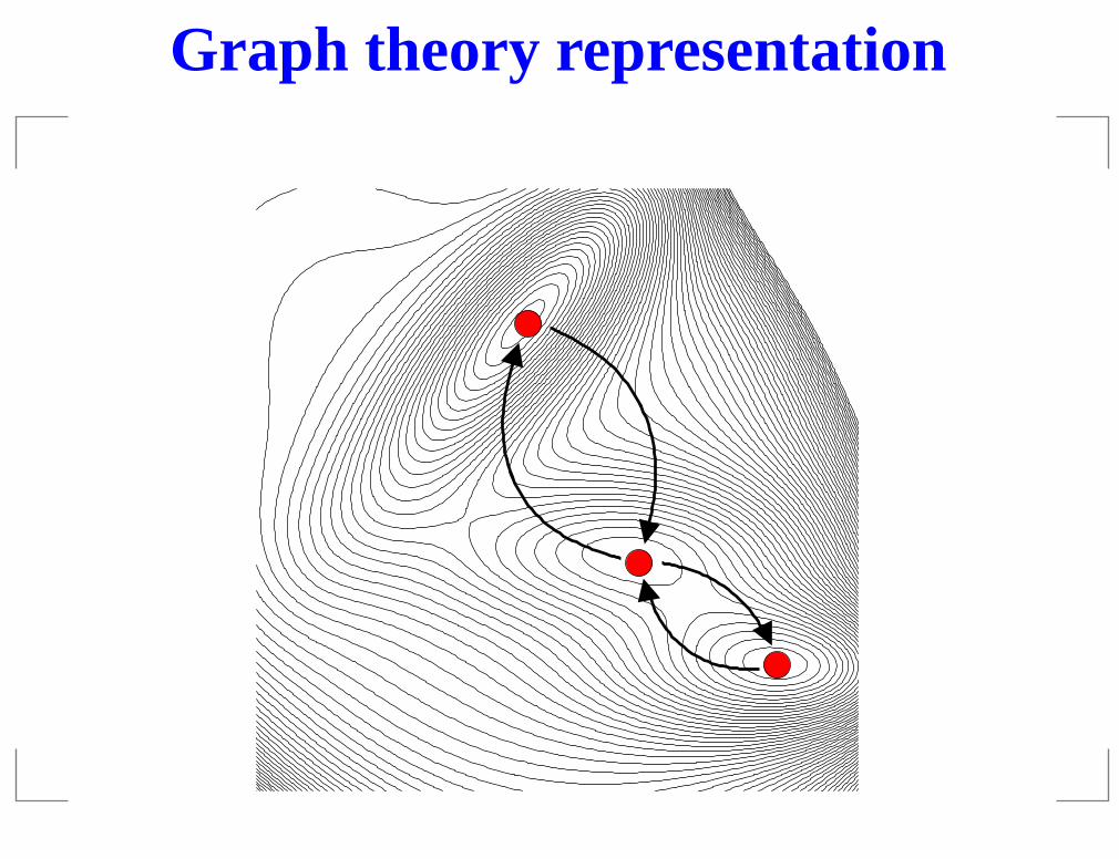
Graph theory representation
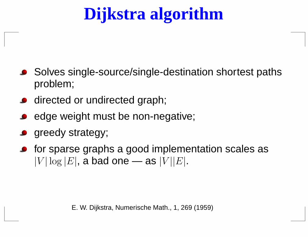
Dijkstra algorithm
Solves single-source/single-destination shortest pathsproblem;
directed or undirected graph;
edge weight must be non-negative;
greedy strategy;
for sparse graphs a good implementation scales as|V | log |E|, a bad one — as |V ||E|.
E. W. Dijkstra, Numerische Math., 1, 269 (1959)
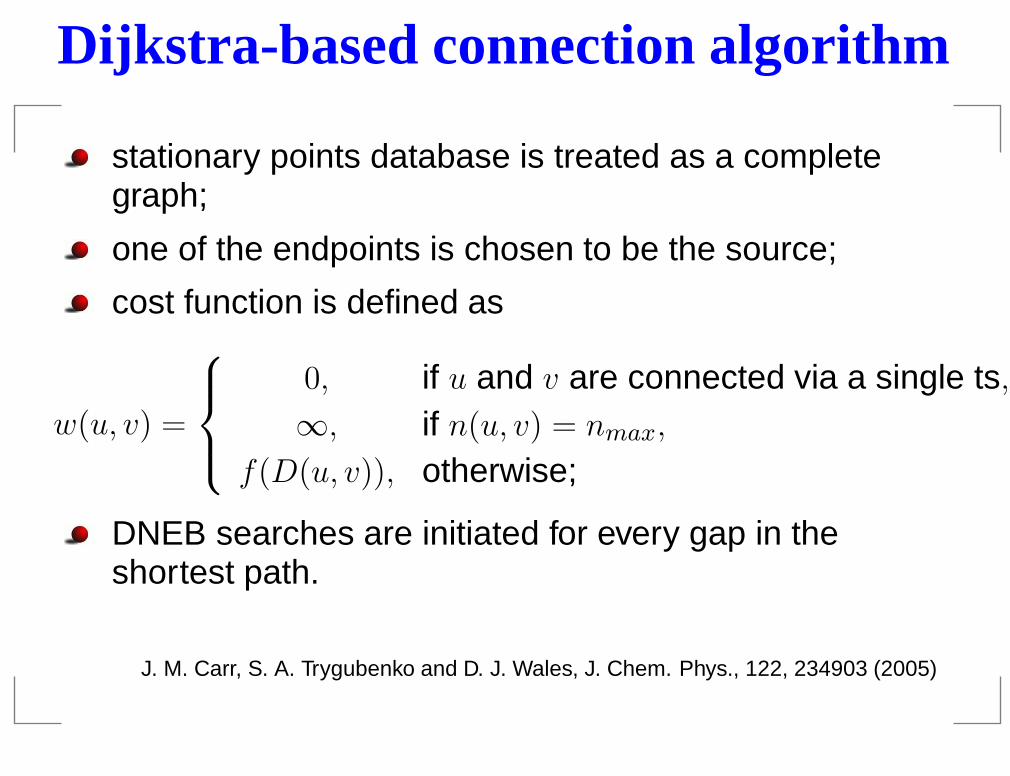
Dijkstra-based connection algorithm
stationary points database is treated as a completegraph;
one of the endpoints is chosen to be the source;
cost function is defined as
w(u, v) =
0, if u and v are connected via a single ts,
∞, if n(u, v) = nmax,
f(D(u, v)), otherwise;
DNEB searches are initiated for every gap in theshortest path.
J. M. Carr, S. A. Trygubenko and D. J. Wales, J. Chem. Phys., 122, 234903 (2005)
A 2D example
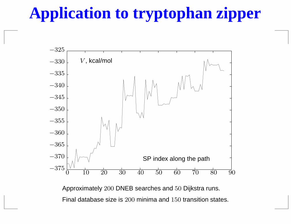
Application to tryptophan zipper
PSfrag replacements
V , kcal/mol
SP index along the path
0 10 20 30 40 50 60 70 80 90
−325
−330
−335
−340
−345
−350
−355
−360
−365
−370
−375
Approximately 200 DNEB searches and 50 Dijkstra runs.
Final database size is 200 minima and 150 transition states.
Summary 3
Graph representation of PES;
Nodes represent minima;
Edges represent transition states;
Dijkstra-based connection algorithm;
Discrete path sampling (DPS) theory;
How to find the fastest pathway?
How to optimise pathway ensemble?
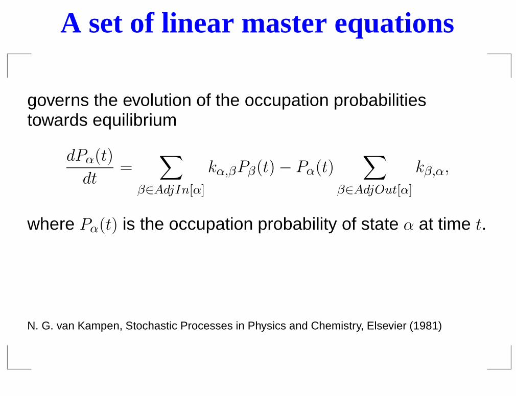
A set of linear master equations
governs the evolution of the occupation probabilitiestowards equilibrium
dPα(t)
dt=
∑
β∈AdjIn[α]
kα,βPβ(t) − Pα(t)∑
β∈AdjOut[α]
kβ,α,
where Pα(t) is the occupation probability of state α at time t.
N. G. van Kampen, Stochastic Processes in Physics and Chemistry, Elsevier (1981)
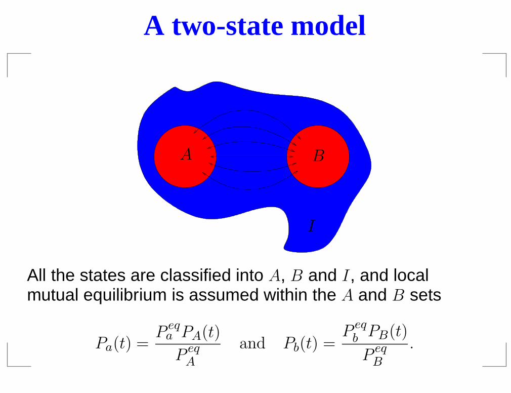
A two-state model
PSfrag replacements
I
A B
All the states are classified into A, B and I, and localmutual equilibrium is assumed within the A and B sets
Pa(t) =P eq
a PA(t)
P eqA
and Pb(t) =P eq
b PB(t)
P eqB
.
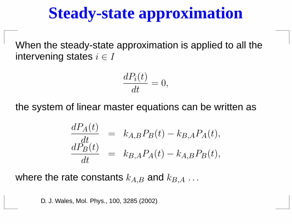
Steady-state approximation
When the steady-state approximation is applied to all theintervening states i ∈ I
dPi(t)
dt= 0,
the system of linear master equations can be written as
dPA(t)
dt= kA,BPB(t) − kB,APA(t),
dPB(t)
dt= kB,APA(t) − kA,BPB(t),
where the rate constants kA,B and kB,A . . .
D. J. Wales, Mol. Phys., 100, 3285 (2002)
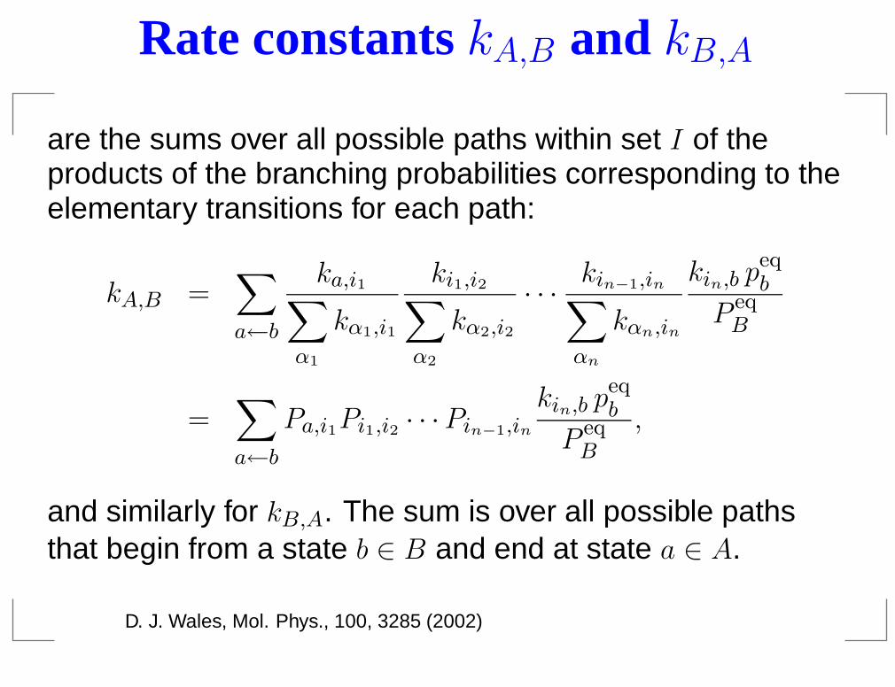
Rate constants kA,B and kB,A
are the sums over all possible paths within set I of theproducts of the branching probabilities corresponding to theelementary transitions for each path:
kA,B =∑
a←b
ka,i1∑
α1
kα1,i1
ki1,i2∑
α2
kα2,i2
· · ·kin−1,in∑
αn
kαn,in
kin,b peqb
P eqB
=∑
a←b
Pa,i1Pi1,i2 · · ·Pin−1,in
kin,b peqb
P eqB
,
and similarly for kB,A. The sum is over all possible pathsthat begin from a state b ∈ B and end at state a ∈ A.
D. J. Wales, Mol. Phys., 100, 3285 (2002)
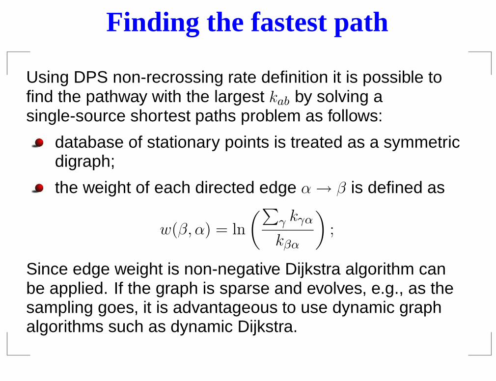
Finding the fastest path
Using DPS non-recrossing rate definition it is possible tofind the pathway with the largest kab by solving asingle-source shortest paths problem as follows:
database of stationary points is treated as a symmetricdigraph;
the weight of each directed edge α → β is defined as
w(β, α) = ln
(∑γ kγα
kβα
);
Since edge weight is non-negative Dijkstra algorithm canbe applied. If the graph is sparse and evolves, e.g., as thesampling goes, it is advantageous to use dynamic graphalgorithms such as dynamic Dijkstra.
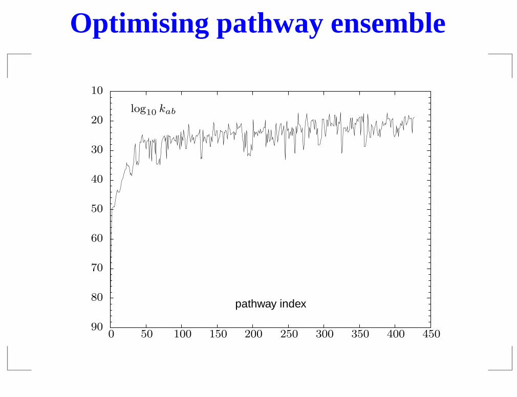
Optimising pathway ensemble
PSfrag replacements
log10 kab
pathway index
0 50 100 150 200 250 300 350 400 450
10
20
30
40
50
60
70
80
90
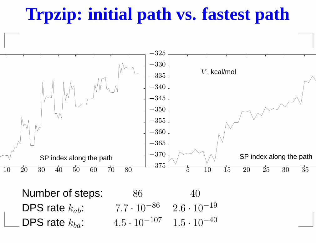
Trpzip: initial path vs. fastest path
PSfrag replacements
V , kcal/mol
SP index along the pathSP index along the path
510 10 1520 20 2530 30 3540 4050 60 70 80
−325
−330
−335
−340
−345
−350
−355
−360
−365
−370
−375
Number of steps: 86 40
DPS rate kab: 7.7 · 10−86 2.6 · 10−19
DPS rate kba: 4.5 · 10−107 1.5 · 10−40
Summary 4
Graph theory tools are very useful in studing PES;
Breadth-first search can be used to find the shortestpathway in linear time;
Discrete path sampling allows to associate a rateconstant with discrete pathway;
Adopting DPS non-recrossing rates and our definition ofthe cost function the fastest path can be identified withDijkstra algorithm in |V | log |E| time. Previously in ourgroup we were using Bellman-Ford algorithm for thispurpose;
Pathway ensemble can be optimised utilising thisinformation.
How to augment DPS rate with recrossings?
Chapman-Kolmogorov equations
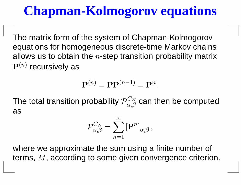
The matrix form of the system of Chapman-Kolmogorovequations for homogeneous discrete-time Markov chainsallows us to obtain the n-step transition probability matrixP(n) recursively as
P(n) = PP(n−1) = Pn.
The total transition probability PCN
α,β can then be computedas
PCN
α,β =∞∑
n=1
[Pn]α,β ,
where we approximate the sum using a finite number ofterms, M , according to some given convergence criterion.
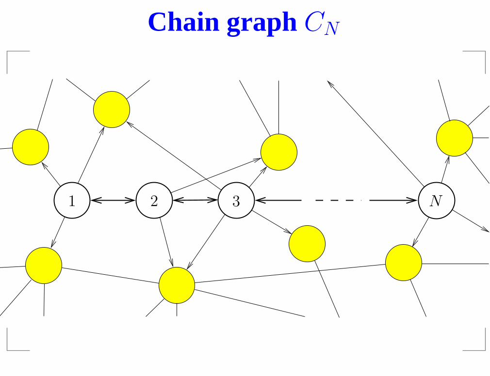
Chain graph CN
PSfrag replacements
1 2 3 N
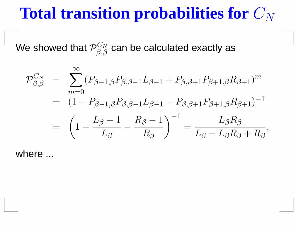
Total transition probabilities for CN
We showed that PCN
β,β can be calculated exactly as
PCN
β,β =
∞∑
m=0
(Pβ−1,βPβ,β−1Lβ−1 + Pβ,β+1Pβ+1,βRβ+1)m
= (1 − Pβ−1,βPβ,β−1Lβ−1 − Pβ,β+1Pβ+1,βRβ+1)−1
=
(1 −
Lβ − 1
Lβ−
Rβ − 1
Rβ
)−1
=LβRβ
Lβ − LβRβ + Rβ,
where ...
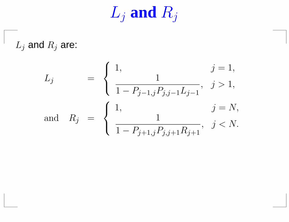
Lj and Rj
Lj and Rj are:
Lj =
1, j = 1,1
1 − Pj−1,jPj,j−1Lj−1, j > 1,
and Rj =
1, j = N,1
1 − Pj+1,jPj,j+1Rj+1, j < N.
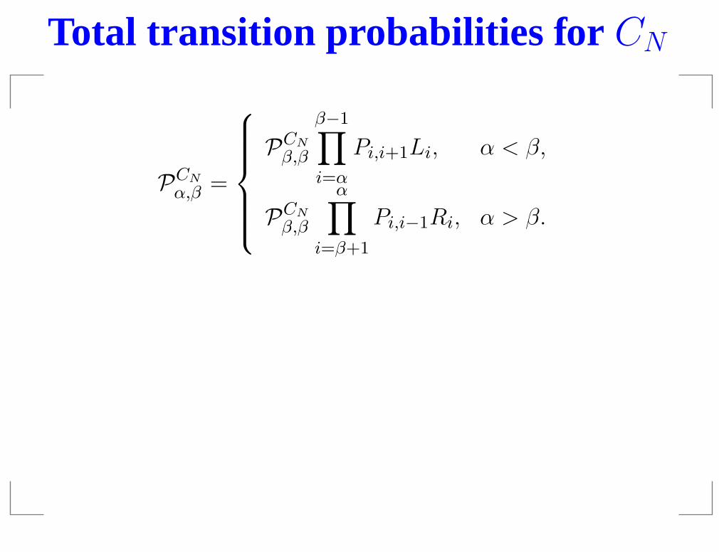
Total transition probabilities for CN
PCN
α,β =
PCN
β,β
β−1∏
i=α
Pi,i+1Li, α < β,
PCN
β,β
α∏
i=β+1
Pi,i−1Ri, α > β.
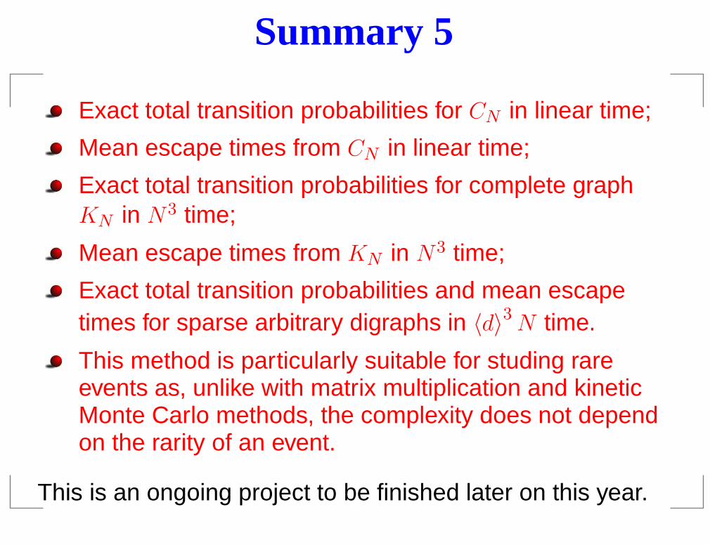
Summary 5
Exact total transition probabilities for CN in linear time;
Mean escape times from CN in linear time;
Exact total transition probabilities for complete graphKN in N3 time;
Mean escape times from KN in N3 time;
Exact total transition probabilities and mean escapetimes for sparse arbitrary digraphs in 〈d〉3 N time.
This method is particularly suitable for studing rareevents as, unlike with matrix multiplication and kineticMonte Carlo methods, the complexity does not dependon the rarity of an event.
This is an ongoing project to be finished later on this year.
Special thanks to
Dr. David Wales, Dr. Catherine Pitt, Tetyana Bogdan, Dr.Joanne Carr, Prof. Petro Holod, Prof. Dmytro Hovorun,Prof. Pavel Hobza, Dr. David Evans, Dr. Viktor Kuprievychand Dr. Igor Anisimov
Kyiv-Mohyla Academy, Ukraine
and you for your attention!