Part IV Statistical Inference - Uwasalipas.uwasa.fi/~sjp/Teaching/ecm/lectures/ecmc4.pdf · Part IV...
54
Statistical Inference Part IV Statistical Inference As of Oct 2, 2019 Seppo Pynn¨ onen Econometrics I
Transcript of Part IV Statistical Inference - Uwasalipas.uwasa.fi/~sjp/Teaching/ecm/lectures/ecmc4.pdf · Part IV...
Statistical Inference
Part IV
Statistical Inference
As of Oct 2, 2019Seppo Pynnonen Econometrics I
Statistical Inference
Sampling Distributions of the OLS Estimator
1 Statistical Inference
Sampling Distributions of the OLS Estimator
Testing for single population coefficients, the t-test
Testing Against One-Sided Alternatives
Two-Sided Alternatives
Other Hypotheses About βj
p-values
Economic, or Practical, versus Statistical Significance
Confidence Intervals for the Coefficients
Simultaneous Testing for Multiple Coefficients, The F -test
Testing General Linear Restrictions
On Reporting the Regression Results
Seppo Pynnonen Econometrics I
Statistical Inference
Sampling Distributions of the OLS Estimator
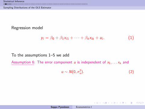
Regression model
yi = β0 + β1xi1 + · · ·+ βkxik + ui . (1)
To the assumptions 1–5 we add
Assumption 6: The error component u is independent of x1, . . . xk and
u ∼ N(0, σ2u). (2)
Seppo Pynnonen Econometrics I
Statistical Inference
Sampling Distributions of the OLS Estimator
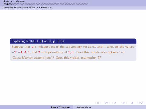
Exploring further 4.1 (W 5e, p. 113)
Suppose that u is independent of the explanatory variables, and it takes on the values
−2, −1, 0, 1, and 2 with probability of 1/5. Does this violate assumptions 1–5
(Gauss-Markov assumptions)? Does this violate assumption 6?
Seppo Pynnonen Econometrics I
Statistical Inference
Sampling Distributions of the OLS Estimator
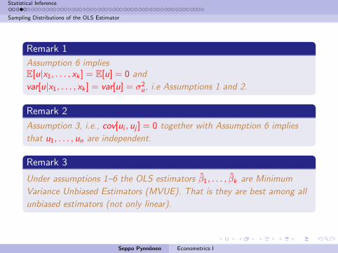
Remark 1
Assumption 6 impliesE[u|x1, . . . , xk ] = E[u] = 0 and
var[u|x1, . . . , xk ] = var[u] = σ2u, i.e Assumptions 1 and 2.
Remark 2
Assumption 3, i.e., cov[ui , uj ] = 0 together with Assumption 6 implies
that u1, . . . , un are independent.
Remark 3
Under assumptions 1–6 the OLS estimators β1, . . . , βk are Minimum
Variance Unbiased Estimators (MVUE). That is they are best among all
unbiased estimators (not only linear).
Seppo Pynnonen Econometrics I
Statistical Inference
Sampling Distributions of the OLS Estimator
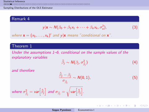
Remark 4
y |x ∼ N(β0 + β1x1 + · · ·+ βkxk , σ2u), (3)
where x = (x1, . . . , xk)′ and y |x means ”conditional on x”.
Theorem 1
Under the assumptions 1–6, conditional on the sample values of theexplanatory variables
βj ∼ N(βj , σ2βj
) (4)
and thereforeβj − βjσβj
∼ N(0, 1), (5)
where σ2βj
= var[βj
]and σβj
=
√var
[βj
].
Seppo Pynnonen Econometrics I
Statistical Inference
Testing for single population coefficients, the t-test
1 Statistical Inference
Sampling Distributions of the OLS Estimator
Testing for single population coefficients, the t-test
Testing Against One-Sided Alternatives
Two-Sided Alternatives
Other Hypotheses About βj
p-values
Economic, or Practical, versus Statistical Significance
Confidence Intervals for the Coefficients
Simultaneous Testing for Multiple Coefficients, The F -test
Testing General Linear Restrictions
On Reporting the Regression Results
Seppo Pynnonen Econometrics I

Statistical Inference
Testing for single population coefficients, the t-test
Theorem 2
Under the assumptions 1–6
βj − βjsβj
∼ tn−k−1, (6)
(the t-distribution with n − k − 1 degrees of freedom) where sβj= se(βj)
and k + 1 is the number of estimated regression coefficients.
Remark 5
The only difference between (5) and (6) is that in the latter the standard
deviation parameter σβjis replaced by its estimator sβj
.
Seppo Pynnonen Econometrics I
Statistical Inference
Testing for single population coefficients, the t-test
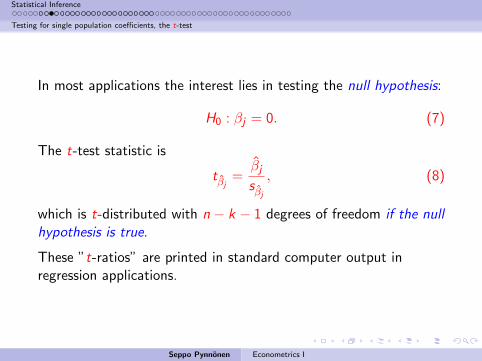
In most applications the interest lies in testing the null hypothesis:
H0 : βj = 0. (7)
The t-test statistic is
tβj =βjsβj, (8)
which is t-distributed with n − k − 1 degrees of freedom if the nullhypothesis is true.
These ”t-ratios” are printed in standard computer output inregression applications.
Seppo Pynnonen Econometrics I
Statistical Inference
Testing for single population coefficients, the t-test
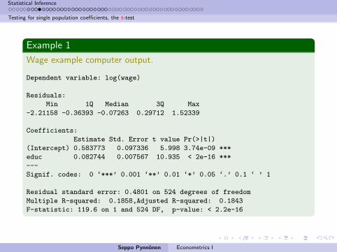
Example 1
Wage example computer output.
Dependent variable: log(wage)
Residuals:
Min 1Q Median 3Q Max
-2.21158 -0.36393 -0.07263 0.29712 1.52339
Coefficients:
Estimate Std. Error t value Pr(>|t|)
(Intercept) 0.583773 0.097336 5.998 3.74e-09 ***
educ 0.082744 0.007567 10.935 < 2e-16 ***
---
Signif. codes: 0 ‘***’ 0.001 ‘**’ 0.01 ‘*’ 0.05 ‘.’ 0.1 ‘ ’ 1
Residual standard error: 0.4801 on 524 degrees of freedom
Multiple R-squared: 0.1858,Adjusted R-squared: 0.1843
F-statistic: 119.6 on 1 and 524 DF, p-value: < 2.2e-16
Seppo Pynnonen Econometrics I
Statistical Inference
Testing for single population coefficients, the t-test
1 Statistical Inference
Sampling Distributions of the OLS Estimator
Testing for single population coefficients, the t-test
Testing Against One-Sided Alternatives
Two-Sided Alternatives
Other Hypotheses About βj
p-values
Economic, or Practical, versus Statistical Significance
Confidence Intervals for the Coefficients
Simultaneous Testing for Multiple Coefficients, The F -test
Testing General Linear Restrictions
On Reporting the Regression Results
Seppo Pynnonen Econometrics I
Statistical Inference
Testing for single population coefficients, the t-test
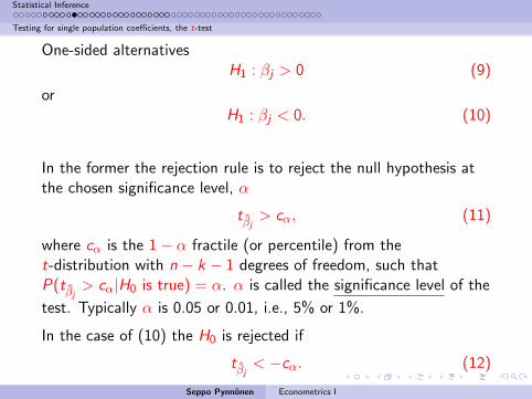
One-sided alternativesH1 : βj > 0 (9)
orH1 : βj < 0. (10)
In the former the rejection rule is to reject the null hypothesis atthe chosen significance level, α
tβj > cα, (11)
where cα is the 1− α fractile (or percentile) from thet-distribution with n − k − 1 degrees of freedom, such thatP(tβj > cα|H0 is true) = α. α is called the significance level of the
test. Typically α is 0.05 or 0.01, i.e., 5% or 1%.
In the case of (10) the H0 is rejected if
tβj < −cα. (12)
These tests are one-tailed test.
Seppo Pynnonen Econometrics I
Statistical Inference
Testing for single population coefficients, the t-test
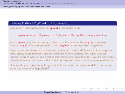
Exploring Further 4.2 (W 5ed, p. 118) (adapted)
Community loan approval rates, apprate, are modeled as
apprate = β0 + β1percmin + β3avginc + β4avgwlth + β5avgdebt + u,
where percmin is the percentage minority in the community, avginc is averageincome, avgwlth is average wealth, and avgdept is average dept obligations.
Suppose we are interested to investigate whether there is difference in loan approvalrates across neighborhoods due to racial and ethnic composition, when averageincome, average wealth, and average dept have been controlled for. We are particularlyinterested in whether there is discrimination against minorities in loan approval rates.
How would you state the null hypothesis in terms of the above model? How do youstate the alternative hypothesis?
Seppo Pynnonen Econometrics I
Statistical Inference
Testing for single population coefficients, the t-test
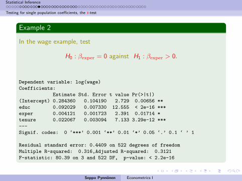
Example 2
In the wage example, test
H0 : βexper = 0 against H1 : βexper > 0.
Dependent variable: log(wage)
Coefficients:
Estimate Std. Error t value Pr(>|t|)
(Intercept) 0.284360 0.104190 2.729 0.00656 **
educ 0.092029 0.007330 12.555 < 2e-16 ***
exper 0.004121 0.001723 2.391 0.01714 *
tenure 0.022067 0.003094 7.133 3.29e-12 ***
---
Signif. codes: 0 ‘***’ 0.001 ‘**’ 0.01 ‘*’ 0.05 ‘.’ 0.1 ‘ ’ 1
Residual standard error: 0.4409 on 522 degrees of freedom
Multiple R-squared: 0.316,Adjusted R-squared: 0.3121
F-statistic: 80.39 on 3 and 522 DF, p-value: < 2.2e-16
Seppo Pynnonen Econometrics I
Statistical Inference
Testing for single population coefficients, the t-test
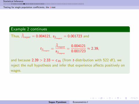
Example 2 continues
Thus, βexper = 0.004121, sβexper= 0.001723 and
tβexper=βexpersβexper
=0.004121
0.001723≈ 2.39,
and because 2.39 > 2.33 = c.01 (from t-distribution with 522 df), we
reject the null hypothesis and infer that experience affects positively on
wages.
Seppo Pynnonen Econometrics I
Statistical Inference
Testing for single population coefficients, the t-test
1 Statistical Inference
Sampling Distributions of the OLS Estimator
Testing for single population coefficients, the t-test
Testing Against One-Sided Alternatives
Two-Sided Alternatives
Other Hypotheses About βj
p-values
Economic, or Practical, versus Statistical Significance
Confidence Intervals for the Coefficients
Simultaneous Testing for Multiple Coefficients, The F -test
Testing General Linear Restrictions
On Reporting the Regression Results
Seppo Pynnonen Econometrics I
Statistical Inference
Testing for single population coefficients, the t-test
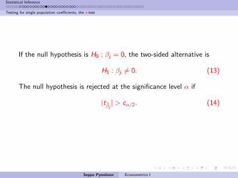
If the null hypothesis is H0 : βj = 0, the two-sided alternative is
H1 : βj 6= 0. (13)
The null hypothesis is rejected at the significance level α if
|tβj | > cα/2. (14)
Seppo Pynnonen Econometrics I
Statistical Inference
Testing for single population coefficients, the t-test
1 Statistical Inference
Sampling Distributions of the OLS Estimator
Testing for single population coefficients, the t-test
Testing Against One-Sided Alternatives
Two-Sided Alternatives
Other Hypotheses About βj
p-values
Economic, or Practical, versus Statistical Significance
Confidence Intervals for the Coefficients
Simultaneous Testing for Multiple Coefficients, The F -test
Testing General Linear Restrictions
On Reporting the Regression Results
Seppo Pynnonen Econometrics I
Statistical Inference
Testing for single population coefficients, the t-test
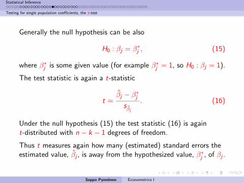
Generally the null hypothesis can be also
H0 : βj = β∗j , (15)
where β∗j is some given value (for example β∗j = 1, so H0 : βj = 1).
The test statistic is again a t-statistic
t =βj − β∗j
sβj. (16)
Under the null hypothesis (15) the test statistic (16) is againt-distributed with n − k − 1 degrees of freedom.
Thus t measures again how many (estimated) standard errors theestimated value, βj , is away from the hypothesized value, β∗j , of βj .
Seppo Pynnonen Econometrics I
Statistical Inference
Testing for single population coefficients, the t-test
The general t statistic is usefully written as
t =(estimate − hypothesized value)
standard error. (17)
Remark 6
The computer print outs always give the t-ratios, i.e., test against zero.
Consequently, they cannot be used to test the more general hypothesis
(15). You can, however, use the standard errors and compute the test
statistics of the form (16).
Seppo Pynnonen Econometrics I

Statistical Inference
Testing for single population coefficients, the t-test
Example 3
Housing prices and air pollution.
A sample of 506 communities in Boston area.Variables:price (y) = median housing pricenox (x1) = nitrogen oxide, parts per 100 mill.dist (x2) = weighted dist. to 5 employ centersrooms (x3) = avg number of rooms per housestratio (x4) = average student-teacher ratio of schools in community
Specified model
log(y) = β0 + β1 log(x1) + β2 log(x2) + β3x3 + β4x4 + u (18)
β1 is the price elasticity of nox. We wish to test
H0 : β1 = −1 against H1 : β1 6= −1
Seppo Pynnonen Econometrics I
Statistical Inference
Testing for single population coefficients, the t-test
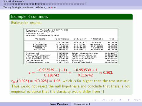
Example 3 continues
Estimation results:
Dependent Variable: LOG(PRICE)Method: Least SquaresSample: 1 506Included observations: 506
Variable Coefficient Std. Error t-Statistic Prob.
C 11.08386 0.318111 34.84271 0.0000LOG(NOX) -0.953539 0.116742 -8.167932 0.0000LOG(DIST) -0.134339 0.043103 -3.116693 0.0019
ROOMS 0.254527 0.018530 13.73570 0.0000STRATIO -0.052451 0.005897 -8.894399 0.0000
R-squared 0.584032 Mean dependent var 9.941057Adjusted R-squared 0.580711 S.D. dependent var 0.409255S.E. of regression 0.265003 Akaike info criterion 0.191679Sum squared resid 35.18346 Schwarz criterion 0.233444Log likelihood -43.49487 F-statistic 175.8552Durbin-Watson stat 0.681595 Prob(F-statistic) 0.000000
t =−0.953539− (−1)
0.116742=−0.953539 + 1
0.116742≈ 0.393.
t501(0.025) ≈ z(0.025) = 1.96, which is far higher than the test statistic.
Thus we do not reject the null hypothesis and conclude that there is not
empirical evidence that the elasticity would differ from -1.
Seppo Pynnonen Econometrics I
Statistical Inference
Testing for single population coefficients, the t-test
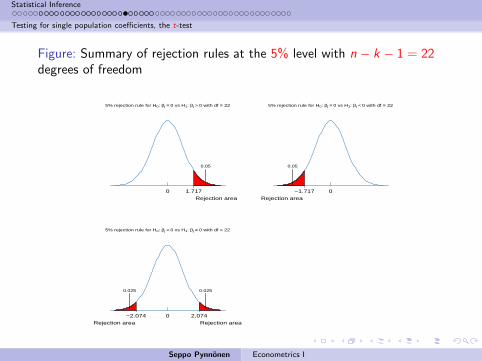
Figure: Summary of rejection rules at the 5% level with n − k − 1 = 22degrees of freedom
5% rejection rule for H0: βj = 0 vs H1: βj > 0 with df = 22
0 1.717Rejection area
0.05
5% rejection rule for H0: βj = 0 vs H1: βj < 0 with df = 22
0−1.717Rejection area
0.05
5% rejection rule for H0: βj = 0 vs H1: βj ≠ 0 with df = 22
0 2.074−2.074Rejection area Rejection area
0.025 0.025
Seppo Pynnonen Econometrics I
Statistical Inference
Testing for single population coefficients, the t-test
1 Statistical Inference
Sampling Distributions of the OLS Estimator
Testing for single population coefficients, the t-test
Testing Against One-Sided Alternatives
Two-Sided Alternatives
Other Hypotheses About βj
p-values
Economic, or Practical, versus Statistical Significance
Confidence Intervals for the Coefficients
Simultaneous Testing for Multiple Coefficients, The F -test
Testing General Linear Restrictions
On Reporting the Regression Results
Seppo Pynnonen Econometrics I
Statistical Inference
Testing for single population coefficients, the t-test
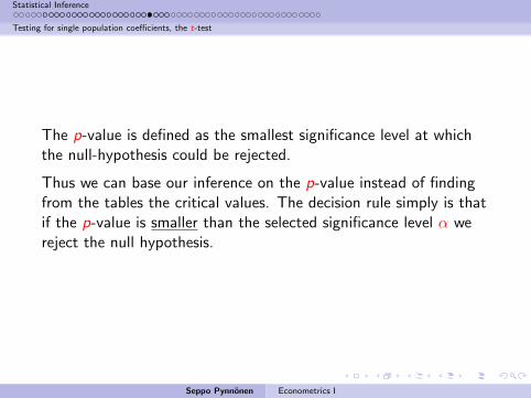
The p-value is defined as the smallest significance level at whichthe null-hypothesis could be rejected.
Thus we can base our inference on the p-value instead of findingfrom the tables the critical values. The decision rule simply is thatif the p-value is smaller than the selected significance level α wereject the null hypothesis.
Seppo Pynnonen Econometrics I
Statistical Inference
Testing for single population coefficients, the t-test
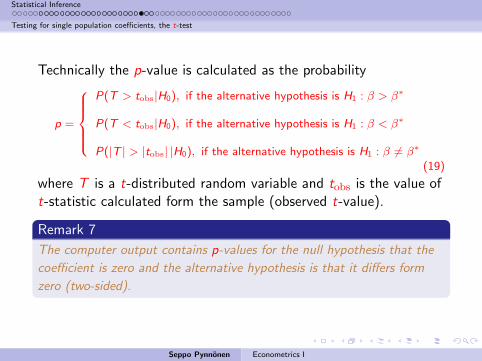
Technically the p-value is calculated as the probability
p =
P(T > tobs|H0), if the alternative hypothesis is H1 : β > β∗
P(T < tobs|H0), if the alternative hypothesis is H1 : β < β∗
P(|T | > |tobs| |H0), if the alternative hypothesis is H1 : β 6= β∗
(19)
where T is a t-distributed random variable and tobs is the value oft-statistic calculated form the sample (observed t-value).
Remark 7
The computer output contains p-values for the null hypothesis that the
coefficient is zero and the alternative hypothesis is that it differs form
zero (two-sided).
Seppo Pynnonen Econometrics I
Statistical Inference
Testing for single population coefficients, the t-test
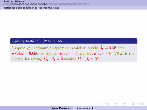
Exploring further 4.3 (W 5e, p. 127)
Suppose you estimate a regression model an obtain β1 = 0.56 and
p-value = 0.086 for testing H0 : β1 = 0 against H1 : β1 6= 0. What is the
p-value for testing H0 : β1 = 0 against H1 : β1 > 0?
Seppo Pynnonen Econometrics I
Statistical Inference
Testing for single population coefficients, the t-test
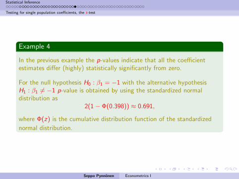
Example 4
In the previous example the p-values indicate that all the coefficientestimates differ (highly) statistically significantly from zero.
For the null hypothesis H0 : β1 = −1 with the alternative hypothesisH1 : β1 6= −1 p-value is obtained by using the standardized normaldistribution as
2(1− Φ(0.398)) ≈ 0.691,
where Φ(z) is the cumulative distribution function of the standardized
normal distribution.
Seppo Pynnonen Econometrics I
Statistical Inference
Economic, or Practical, versus Statistical Significance
1 Statistical Inference
Sampling Distributions of the OLS Estimator
Testing for single population coefficients, the t-test
Testing Against One-Sided Alternatives
Two-Sided Alternatives
Other Hypotheses About βj
p-values
Economic, or Practical, versus Statistical Significance
Confidence Intervals for the Coefficients
Simultaneous Testing for Multiple Coefficients, The F -test
Testing General Linear Restrictions
On Reporting the Regression Results
Seppo Pynnonen Econometrics I
Statistical Inference
Economic, or Practical, versus Statistical Significance
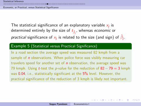
The statistical significance of an explanatory variable xj isdetermined entirely by the size of tβj , whereas economic or
practical significance of xj is related to the size (and sign) of βj .
Example 5 (Statistical versus Practical Significance)
In a road section the average speed was measured 82 kmph from a
sample of n observations. When police force was visibly measuring car
travelers speed for another set of n observation, the average speed was
79 kmph. Using t-test the p-value for the reduction of 82− 79 = 3 kmph
was 0.04, i.e., statistically significant at the 5% level. However, the
practical significance of the reduction of 3 kmph is likely not important.
Seppo Pynnonen Econometrics I
Statistical Inference
Confidence Intervals for the Coefficients
1 Statistical Inference
Sampling Distributions of the OLS Estimator
Testing for single population coefficients, the t-test
Testing Against One-Sided Alternatives
Two-Sided Alternatives
Other Hypotheses About βj
p-values
Economic, or Practical, versus Statistical Significance
Confidence Intervals for the Coefficients
Simultaneous Testing for Multiple Coefficients, The F -test
Testing General Linear Restrictions
On Reporting the Regression Results
Seppo Pynnonen Econometrics I
Statistical Inference
Confidence Intervals for the Coefficients
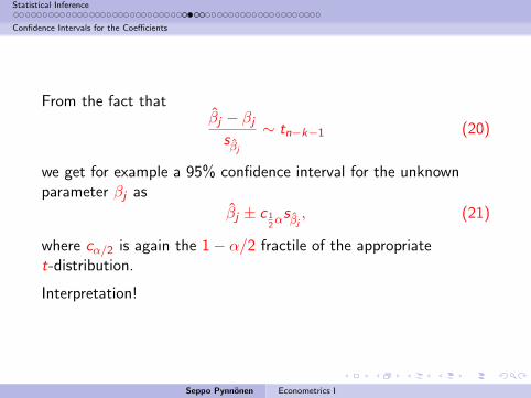
From the fact thatβj − βjsβj
∼ tn−k−1 (20)
we get for example a 95% confidence interval for the unknownparameter βj as
βj ± c 12αsβj , (21)
where cα/2 is again the 1− α/2 fractile of the appropriatet-distribution.
Interpretation!
Seppo Pynnonen Econometrics I
Statistical Inference
Confidence Intervals for the Coefficients
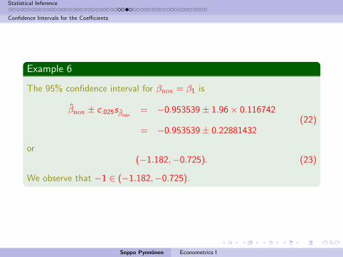
Example 6
The 95% confidence interval for βnox = β1 is
βnox ± c.025sβnox= −0.953539± 1.96× 0.116742
= −0.953539± 0.22881432(22)
or(−1.182,−0.725). (23)
We observe that −1 ∈ (−1.182,−0.725).
Seppo Pynnonen Econometrics I
Statistical Inference
Confidence Intervals for the Coefficients
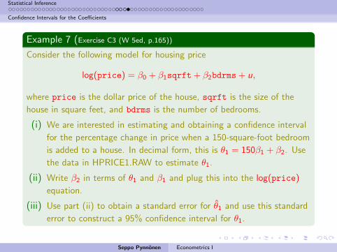
Example 7 (Exercise C3 (W 5ed, p.165))
Consider the following model for housing price
log(price) = β0 + β1sqrft + β2bdrms + u,
where price is the dollar price of the house, sqrft is the size of the
house in square feet, and bdrms is the number of bedrooms.
(i) We are interested in estimating and obtaining a confidence interval
for the percentage change in price when a 150-square-foot bedroom
is added to a house. In decimal form, this is θ1 = 150β1 + β2. Use
the data in HPRICE1.RAW to estimate θ1.
(ii) Write β2 in terms of θ1 and β1 and plug this into the log(price)
equation.
(iii) Use part (ii) to obtain a standard error for θ1 and use this standard
error to construct a 95% confidence interval for θ1.
Seppo Pynnonen Econometrics I
Statistical Inference
Simultaneous Testing for Multiple Coefficients, The F -test
1 Statistical Inference
Sampling Distributions of the OLS Estimator
Testing for single population coefficients, the t-test
Testing Against One-Sided Alternatives
Two-Sided Alternatives
Other Hypotheses About βj
p-values
Economic, or Practical, versus Statistical Significance
Confidence Intervals for the Coefficients
Simultaneous Testing for Multiple Coefficients, The F -test
Testing General Linear Restrictions
On Reporting the Regression Results
Seppo Pynnonen Econometrics I
Statistical Inference
Simultaneous Testing for Multiple Coefficients, The F -test
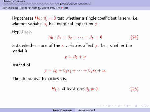
Hypotheses H0 : βj = 0 test whether a single coefficient is zero, i.e.whether variable xj has marginal impact on y .
HypothesisH0 : β1 = β2 = · · · = βk = 0 (24)
tests whether none of the x-variables affect y . I.e., whether themodel is
y = β0 + u
instead ofy = β0 + β1x1 + · · ·+ βkxk + u.
The alternative hypothesis is
H1 : at least one βj 6= 0. (25)
Seppo Pynnonen Econometrics I
Statistical Inference
Simultaneous Testing for Multiple Coefficients, The F -test
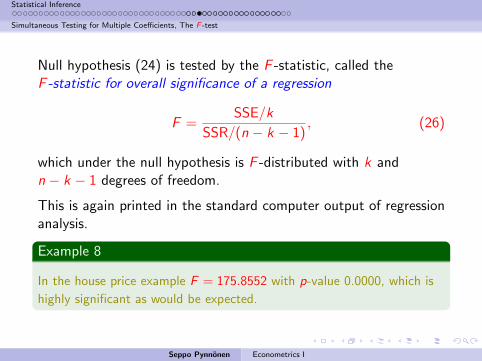
Null hypothesis (24) is tested by the F -statistic, called theF -statistic for overall significance of a regression
F =SSE/k
SSR/(n − k − 1), (26)
which under the null hypothesis is F -distributed with k andn − k − 1 degrees of freedom.
This is again printed in the standard computer output of regressionanalysis.
Example 8
In the house price example F = 175.8552 with p-value 0.0000, which is
highly significant as would be expected.
Seppo Pynnonen Econometrics I
Statistical Inference
Simultaneous Testing for Multiple Coefficients, The F -test
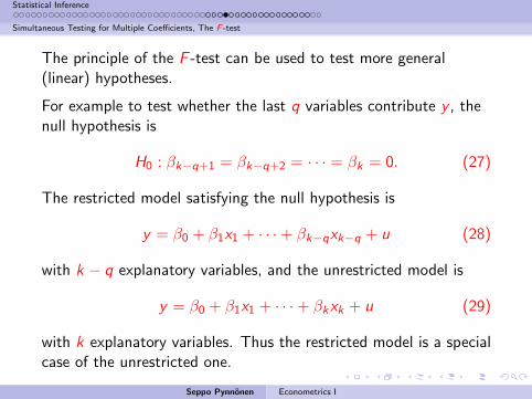
The principle of the F -test can be used to test more general(linear) hypotheses.
For example to test whether the last q variables contribute y , thenull hypothesis is
H0 : βk−q+1 = βk−q+2 = · · · = βk = 0. (27)
The restricted model satisfying the null hypothesis is
y = β0 + β1x1 + · · ·+ βk−qxk−q + u (28)
with k − q explanatory variables, and the unrestricted model is
y = β0 + β1x1 + · · ·+ βkxk + u (29)
with k explanatory variables. Thus the restricted model is a specialcase of the unrestricted one.
Seppo Pynnonen Econometrics I
Statistical Inference
Simultaneous Testing for Multiple Coefficients, The F -test
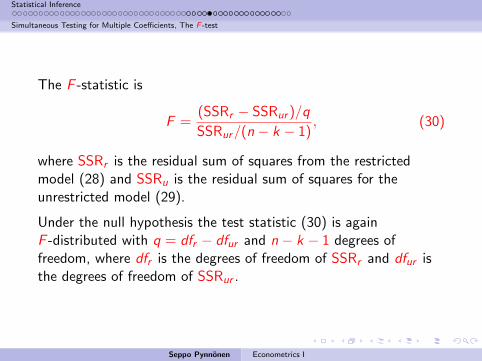
The F -statistic is
F =(SSRr − SSRur )/q
SSRur/(n − k − 1), (30)
where SSRr is the residual sum of squares from the restrictedmodel (28) and SSRu is the residual sum of squares for theunrestricted model (29).
Under the null hypothesis the test statistic (30) is againF -distributed with q = dfr − dfur and n − k − 1 degrees offreedom, where dfr is the degrees of freedom of SSRr and dfur isthe degrees of freedom of SSRur .
Seppo Pynnonen Econometrics I

Statistical Inference
Simultaneous Testing for Multiple Coefficients, The F -test
Remark 8
Testing for a single coefficient is a special case of (27), and it can be
shown that in such a case the F -statistic from (30) equals t2βj
.
Remark 9
It can be easily shown that
F =(R2
ur − R2r )/q
(1− R2ur )/(n − k − 1)
, (31)
where R2ur and R2
r are the R-squares of the unrestricted and restricted
models, respectively.
Seppo Pynnonen Econometrics I
Statistical Inference
Simultaneous Testing for Multiple Coefficients, The F -test
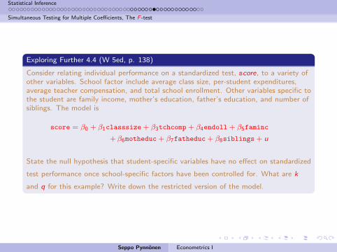
Exploring Further 4.4 (W 5ed, p. 138)
Consider relating individual performance on a standardized test, score, to a variety ofother variables. School factor include average class size, per-student expenditures,average teacher compensation, and total school enrollment. Other variables specific tothe student are family income, mother’s education, father’s education, and number ofsiblings. The model is
score = β0 + β1classsize + β3tchcomp + β4endoll + β5faminc
+β6motheduc + β7fatheduc + β8siblings + u
State the null hypothesis that student-specific variables have no effect on standardized
test performance once school-specific factors have been controlled for. What are k
and q for this example? Write down the restricted version of the model.
Seppo Pynnonen Econometrics I
Statistical Inference
Simultaneous Testing for Multiple Coefficients, The F -test
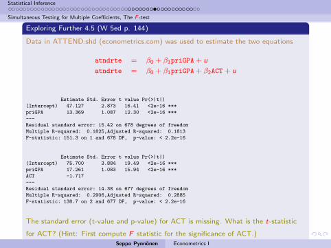
Exploring Further 4.5 (W 5ed p. 144)
Data in ATTEND.shd (econometrics.com) was used to estimate the two equations
atndrte = β0 + β1priGPA + u
atndrte = β0 + β1priGPA + β2ACT + u
Estimate Std. Error t value Pr(>|t|)
(Intercept) 47.127 2.873 16.41 <2e-16 ***
priGPA 13.369 1.087 12.30 <2e-16 ***
---
Residual standard error: 15.42 on 678 degrees of freedom
Multiple R-squared: 0.1825,Adjusted R-squared: 0.1813
F-statistic: 151.3 on 1 and 678 DF, p-value: < 2.2e-16
Estimate Std. Error t value Pr(>|t|)
(Intercept) 75.700 3.884 19.49 <2e-16 ***
priGPA 17.261 1.083 15.94 <2e-16 ***
ACT -1.717
---
Residual standard error: 14.38 on 677 degrees of freedom
Multiple R-squared: 0.2906,Adjusted R-squared: 0.2885
F-statistic: 138.7 on 2 and 677 DF, p-value: < 2.2e-16
The standard error (t-value and p-value) for ACT is missing. What is the t-statistic
for ACT? (Hint: First compute F statistic for the significance of ACT.)
Seppo Pynnonen Econometrics I
Statistical Inference
Simultaneous Testing for Multiple Coefficients, The F -test
1 Statistical Inference
Sampling Distributions of the OLS Estimator
Testing for single population coefficients, the t-test
Testing Against One-Sided Alternatives
Two-Sided Alternatives
Other Hypotheses About βj
p-values
Economic, or Practical, versus Statistical Significance
Confidence Intervals for the Coefficients
Simultaneous Testing for Multiple Coefficients, The F -test
Testing General Linear Restrictions
On Reporting the Regression Results
Seppo Pynnonen Econometrics I
Statistical Inference
Simultaneous Testing for Multiple Coefficients, The F -test
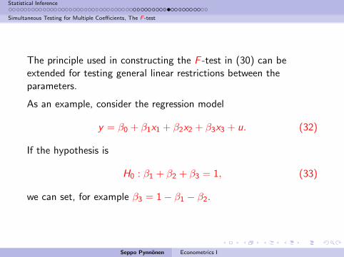
The principle used in constructing the F -test in (30) can beextended for testing general linear restrictions between theparameters.
As an example, consider the regression model
y = β0 + β1x1 + β2x2 + β3x3 + u. (32)
If the hypothesis is
H0 : β1 + β2 + β3 = 1, (33)
we can set, for example β3 = 1− β1 − β2.
Seppo Pynnonen Econometrics I
Statistical Inference
Simultaneous Testing for Multiple Coefficients, The F -test
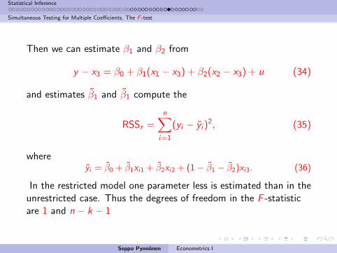
Then we can estimate β1 and β2 from
y − x3 = β0 + β1(x1 − x3) + β2(x2 − x3) + u (34)
and estimates β1 and β1 compute the
RSSr =n∑
i=1
(yi − yi )2, (35)
whereyi = β0 + β1xi1 + β2xi2 + (1− β1 − β2)xi3. (36)
In the restricted model one parameter less is estimated than in theunrestricted case. Thus the degrees of freedom in the F -statisticare 1 and n − k − 1
Seppo Pynnonen Econometrics I
Statistical Inference
Simultaneous Testing for Multiple Coefficients, The F -test
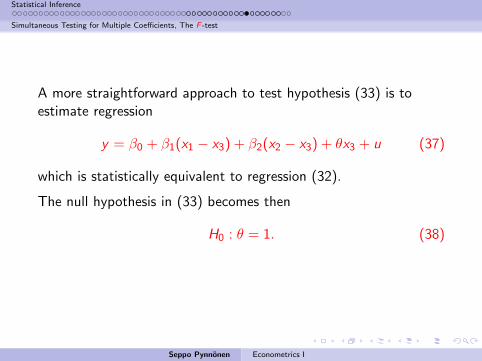
A more straightforward approach to test hypothesis (33) is toestimate regression
y = β0 + β1(x1 − x3) + β2(x2 − x3) + θx3 + u (37)
which is statistically equivalent to regression (32).
The null hypothesis in (33) becomes then
H0 : θ = 1. (38)
Seppo Pynnonen Econometrics I
Statistical Inference
Simultaneous Testing for Multiple Coefficients, The F -test
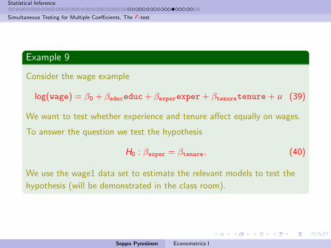
Example 9
Consider the wage example
log(wage) = β0 + βeduceduc + βexperexper + βtenuretenure + u (39)
We want to test whether experience and tenure affect equally on wages.
To answer the question we test the hypothesis
H0 : βexper = βtenure. (40)
We use the wage1 data set to estimate the relevant models to test the
hypothesis (will be demonstrated in the class room).
Seppo Pynnonen Econometrics I
Statistical Inference
Simultaneous Testing for Multiple Coefficients, The F -test
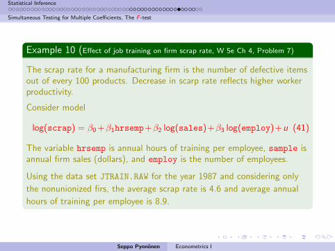
Example 10 (Effect of job training on firm scrap rate, W 5e Ch 4, Problem 7)
The scrap rate for a manufacturing firm is the number of defective itemsout of every 100 products. Decrease in scarp rate reflects higher workerproductivity.
Consider model
log(scrap) = β0 +β1hrsemp+β2 log(sales)+β3 log(employ)+u (41)
The variable hrsemp is annual hours of training per employee, sample isannual firm sales (dollars), and employ is the number of employees.
Using the data set JTRAIN.RAW for the year 1987 and considering only
the nonunionized firs, the average scrap rate is 4.6 and average annual
hours of training per employee is 8.9.
Seppo Pynnonen Econometrics I
Statistical Inference
Simultaneous Testing for Multiple Coefficients, The F -test
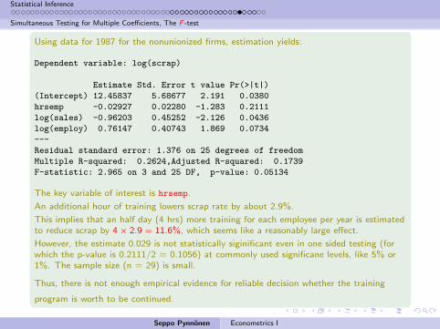
Using data for 1987 for the nonunionized firms, estimation yields:
Dependent variable: log(scrap)
Estimate Std. Error t value Pr(>|t|)
(Intercept) 12.45837 5.68677 2.191 0.0380
hrsemp -0.02927 0.02280 -1.283 0.2111
log(sales) -0.96203 0.45252 -2.126 0.0436
log(employ) 0.76147 0.40743 1.869 0.0734
---
Residual standard error: 1.376 on 25 degrees of freedom
Multiple R-squared: 0.2624,Adjusted R-squared: 0.1739
F-statistic: 2.965 on 3 and 25 DF, p-value: 0.05134
The key variable of interest is hrsemp.
An additional hour of training lowers scrap rate by about 2.9%.
This implies that an half day (4 hrs) more training for each employee per year is estimatedto reduce scrap by 4 × 2.9 = 11.6%, which seems like a reasonably large effect.
However, the estimate 0.029 is not statistically siginificant even in one sided testing (forwhich the p-value is 0.2111/2 = 0.1056) at commonly used significane levels, like 5% or1%. The sample size (n = 29) is small.
Thus, there is not enough empirical evidence for reliable decision whether the training
program is worth to be continued.
Seppo Pynnonen Econometrics I
Statistical Inference
Simultaneous Testing for Multiple Coefficients, The F -test
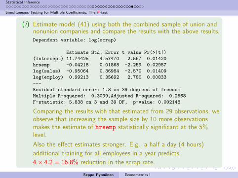
(i) Estimate model (41) using both the combined sample of union andnonunion companies and compare the results with the above results.Dependent variable: log(scrap)
Estimate Std. Error t value Pr(>|t|)
(Intercept) 11.74425 4.57470 2.567 0.01420
hrsemp -0.04218 0.01868 -2.259 0.02957
log(sales) -0.95064 0.36984 -2.570 0.01409
log(employ) 0.99213 0.35692 2.780 0.00833
---
Residual standard error: 1.3 on 39 degrees of freedom
Multiple R-squared: 0.3099,Adjusted R-squared: 0.2568
F-statistic: 5.838 on 3 and 39 DF, p-value: 0.002148
Comparing the results with that estimated from 29 observations, weobserve that increasing the sample size by 10 more observationsmakes the estimate of hrsemp statistically significant at the 5%level.
Also the effect estimates stronger. E.g., a half a day (4 hours)
additional training for all employees in a year predicts
4× 4.2 = 16.8% reduction in the scrap rate.
Seppo Pynnonen Econometrics I
Statistical Inference
Simultaneous Testing for Multiple Coefficients, The F -test
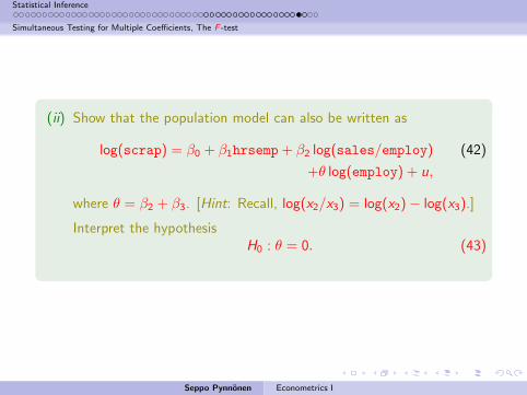
(ii) Show that the population model can also be written as
log(scrap) = β0 + β1hrsemp + β2 log(sales/employ) (42)
+θ log(employ) + u,
where θ = β2 + β3. [Hint: Recall, log(x2/x3) = log(x2)− log(x3).]
Interpret the hypothesisH0 : θ = 0. (43)
Seppo Pynnonen Econometrics I
Statistical Inference
Simultaneous Testing for Multiple Coefficients, The F -test
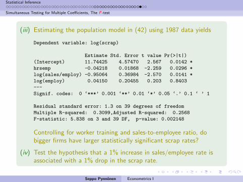
(iii) Estimating the population model in (42) using 1987 data yields
Dependent variable: log(scrap)
Estimate Std. Error t value Pr(>|t|)
(Intercept) 11.74425 4.57470 2.567 0.0142 *
hrsemp -0.04218 0.01868 -2.259 0.0296 *
log(sales/employ) -0.95064 0.36984 -2.570 0.0141 *
log(employ) 0.04150 0.20455 0.203 0.8403
---
Signif. codes: 0 ‘***’ 0.001 ‘**’ 0.01 ‘*’ 0.05 ‘.’ 0.1 ‘ ’ 1
Residual standard error: 1.3 on 39 degrees of freedom
Multiple R-squared: 0.3099,Adjusted R-squared: 0.2568
F-statistic: 5.838 on 3 and 39 DF, p-value: 0.002148
Controlling for worker training and sales-to-employee ratio, dobigger firms have larger statistically significant scrap rates?
(iv) Test the hypothesis that a 1% increase in sales/employee rate isassociated with a 1% drop in the scrap rate.
Seppo Pynnonen Econometrics I
Statistical Inference
On Reporting the Regression Results
1 Statistical Inference
Sampling Distributions of the OLS Estimator
Testing for single population coefficients, the t-test
Testing Against One-Sided Alternatives
Two-Sided Alternatives
Other Hypotheses About βj
p-values
Economic, or Practical, versus Statistical Significance
Confidence Intervals for the Coefficients
Simultaneous Testing for Multiple Coefficients, The F -test
Testing General Linear Restrictions
On Reporting the Regression Results
Seppo Pynnonen Econometrics I
Statistical Inference
On Reporting the Regression Results
(1) Estimated coefficients and interpret them
(2) Standard errors (or t-ratios or p-values)
(3) R-squared and number of observations
(4) Optionally, standard error of regression
Seppo Pynnonen Econometrics I