6

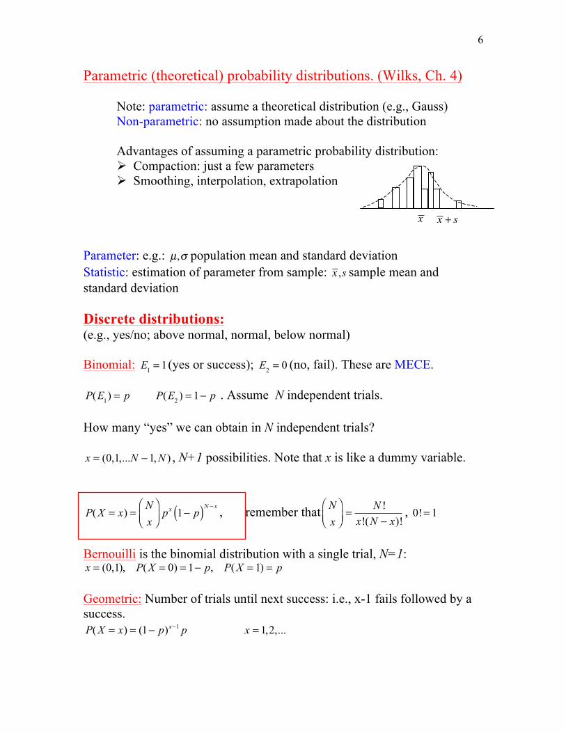
Parametric (theoretical) probability distributions. (Wilks, Ch. 4) Note: parametric: assume a theoretical distribution (e.g., Gauss) Non-parametric: no assumption made about the distribution Advantages of assuming a parametric probability distribution: Compaction: just a few parameters Smoothing, interpolation, extrapolation

Parameter: e.g.: µ,σ population mean and standard deviation Statistic: estimation of parameter from sample: x ,s sample mean and standard deviation Discrete distributions: (e.g., yes/no; above normal, normal, below normal) Binomial: E1 = 1(yes or success); E2 = 0 (no, fail). These are MECE.

P(E1) = p P(E2 ) = 1− p . Assume N independent trials. How many “yes” we can obtain in N independent trials? x = (0,1,...N −1, N ) , N+1 possibilities. Note that x is like a dummy variable.

P( X = x) =

Nx

⎛⎝⎜

⎞⎠⎟

px 1− p( )N − x , remember that

Nx

⎛⎝⎜

⎞⎠⎟=

N !x!(N − x)!

, 0!= 1

Bernouilli is the binomial distribution with a single trial, N=1: x = (0,1), P( X = 0) = 1− p, P( X = 1) = p Geometric: Number of trials until next success: i.e., x-1 fails followed by a success. P( X = x) = (1− p)x−1 p x = 1,2,...

x

x s+

7

Poisson: Approximation of binomial for small p and large N. Events occur randomly at a constant rate (per N trials) µ = Np . The rate per trial p is low so that events in the same period (N trials) are approximately independent. Example: assume the probability of a tornado in a certain county on a given day is p=1/100. Then the average rate per season is: µ = 90 *1 / 100 = 0.9 .

P( X = x) =

µ xe−µ

x!x = 0,1,2...

Question: What is the probability of having 0 tornados, 1 or 2 tornados in a season? Expected Value: “probability weighted mean”

Example: Expected mean: µ = E( X ) = x.P( X = x)

x∑

Example: Binomial distrib. mean µ = E( X ) = x

x=0

N

∑ Nx

⎛⎝⎜

⎞⎠⎟

px (1− p)1− x = Np

Properties of expected value:

E( f ( X )) = f (x).P( X = x);

x∑ E(a. f ( X ) + b.g( X )) = a.E( f ( X )) + b.E(g( X ))

Example Variance

Var( X ) = E(( X − µ)2 ) = (x − µ)2

x∑ P( X = x) =

= x2

x∑ P( X = x) − 2µ x

x∑ P( X = x) + µ2 P( X = x) = E( X 2 ) −

x∑ µ2

E.g.: Binomial: Var( X ) = Np(1− p)

Geometric: Var( X ) =

(1− p)p2

Poisson: Var( X ) = Np = µ

8

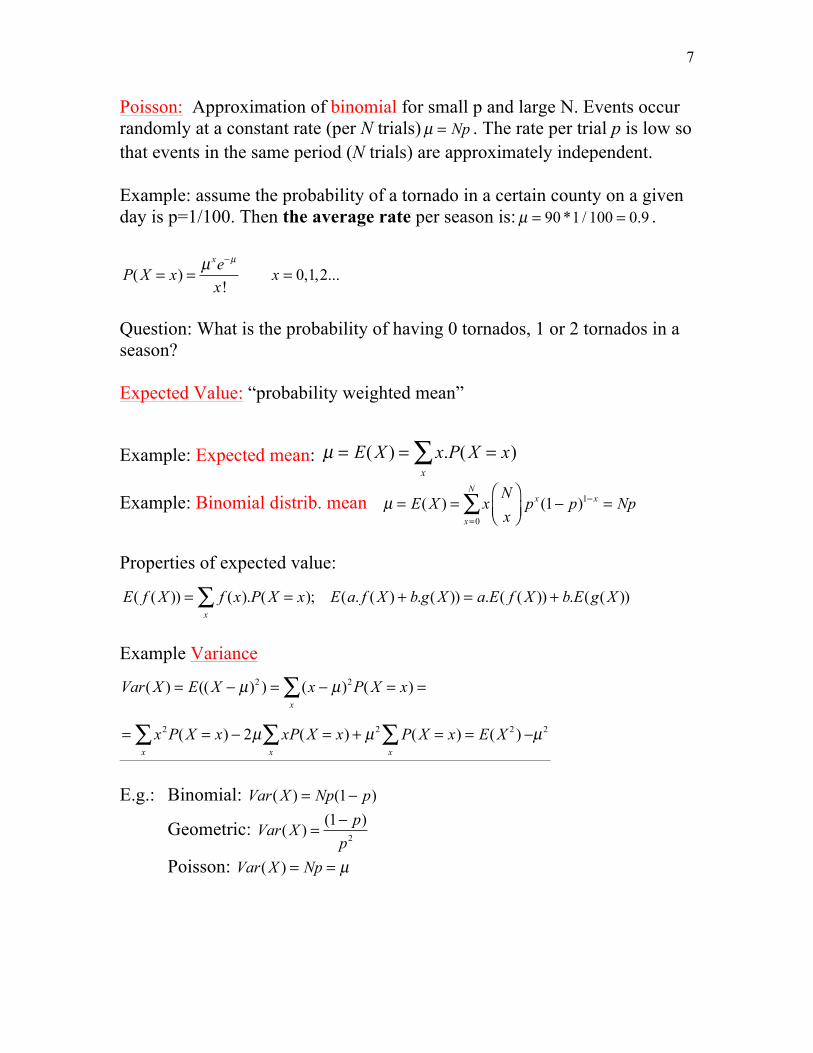
Continuous probability distributions Probability density function f(x): PDF

f (x)dx ≡ 1∫

f (x)dx = P(| X − x |< δ )

x−δ

x+δ

∫ x − δ x x + δ

Cumulative prob distribution function (CDF)

F(a) = P( X ≤ a) = f (x)dx

x≤a∫

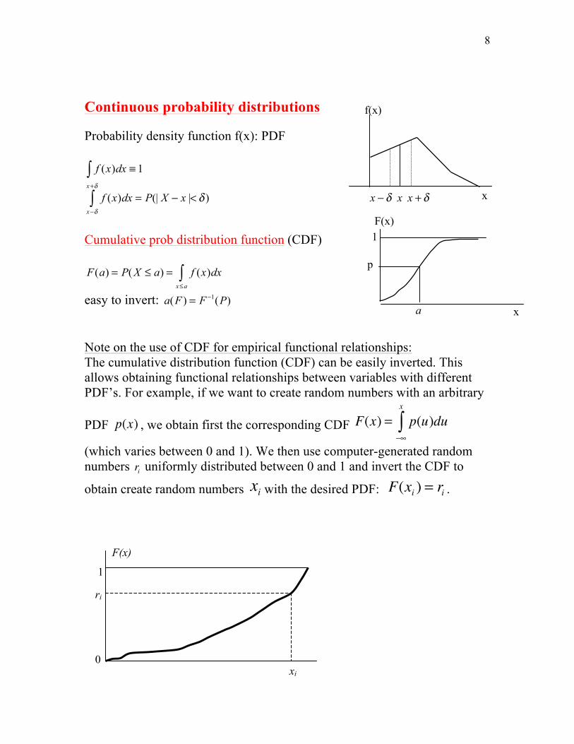
easy to invert: a(F ) = F −1(P) Note on the use of CDF for empirical functional relationships: The cumulative distribution function (CDF) can be easily inverted. This allows obtaining functional relationships between variables with different PDF’s. For example, if we want to create random numbers with an arbitrary

PDF p(x) , we obtain first the corresponding CDF F(x) = p(u)du−∞

x

∫

(which varies between 0 and 1). We then use computer-generated random numbers ri uniformly distributed between 0 and 1 and invert the CDF to

obtain create random numbers xi with the desired PDF: F(xi ) = ri .

f(x)

x

F(x) 1

p

x a

F(x)

1

0

ri

xi

9

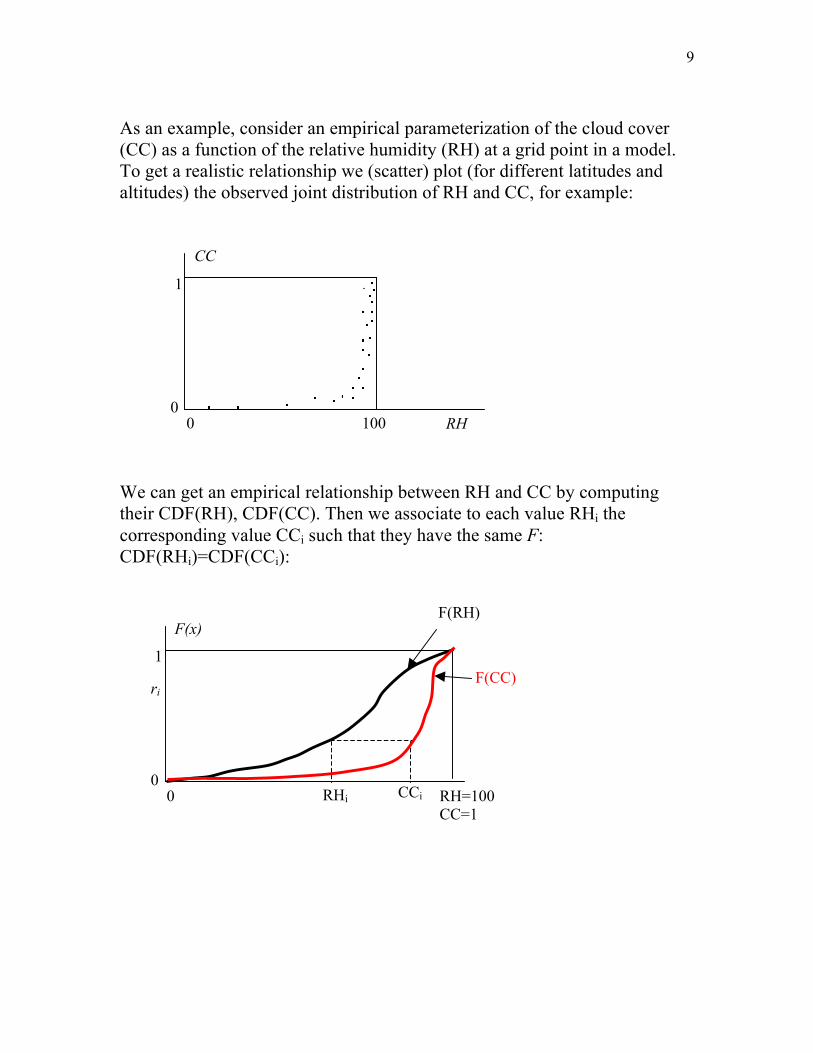
As an example, consider an empirical parameterization of the cloud cover (CC) as a function of the relative humidity (RH) at a grid point in a model. To get a realistic relationship we (scatter) plot (for different latitudes and altitudes) the observed joint distribution of RH and CC, for example: We can get an empirical relationship between RH and CC by computing their CDF(RH), CDF(CC). Then we associate to each value RHi the corresponding value CCi such that they have the same F: CDF(RHi)=CDF(CCi):

CC

1

0 RH 0 100

F(x)

1

0

ri

RH=100 CC=1

0

F(RH)

F(CC)

RHi CCi

10

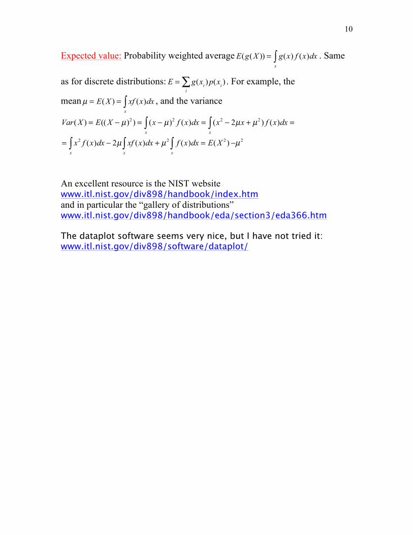
Expected value: Probability weighted average E(g( X )) = g(x) f (x)dx

x∫ . Same

as for discrete distributions: E = g(xi ) p(xi )

i∑ . For example, the

mean µ = E( X ) = xf (x)dx

x∫ , and the variance

Var( X ) = E(( X − µ)2 ) = (x − µ)2 f (x)dxx∫ = (x2 − 2µx + µ2 ) f (x)dx

x∫ =

= x2 f (x)dx − 2µ xf (x)dxx∫ + µ2 f (x)dx

x∫ = E( X 2 ) −

x∫ µ2

An excellent resource is the NIST website www.itl.nist.gov/div898/handbook/index.htm and in particular the “gallery of distributions” www.itl.nist.gov/div898/handbook/eda/section3/eda366.htm The dataplot software seems very nice, but I have not tried it: www.itl.nist.gov/div898/software/dataplot/

11

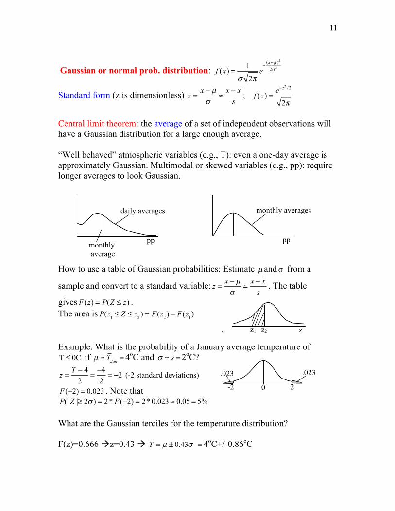
Gaussian or normal prob. distribution: f (x) =

1σ 2π

e−

( x−µ )2

2σ 2

Standard form (z is dimensionless) z =

x − µσ

≈x − x

s; f (z) =

e− z2 / 2

2π

Central limit theorem: the average of a set of independent observations will have a Gaussian distribution for a large enough average. “Well behaved” atmospheric variables (e.g., T): even a one-day average is approximately Gaussian. Multimodal or skewed variables (e.g., pp): require longer averages to look Gaussian. How to use a table of Gaussian probabilities: Estimate µ andσ from a

sample and convert to a standard variable: z =

x − µσ

x − xs

. The table

gives F(z) = P(Z ≤ z) . The area is P(z1 ≤ Z ≤ z2 ) = F(z2 ) − F(z1) Example: What is the probability of a January average temperature of T ≤ 0C if µ TJan = 4oC and σ s = 2oC?

z = T − 4

2=−42

= −2 (-2 standard deviations)

F(−2) = 0.023 . Note that P(| Z |≥ 2σ ) = 2 * F(−2) = 2 *0.023 0.05 = 5% What are the Gaussian terciles for the temperature distribution? F(z)=0.666 z=0.43 T = µ ± 0.43σ = 4oC+/-0.86oC

daily averages

pp monthly average

monthly averages

pp

z2 z1 z

-2 2

.023 .023

0

12

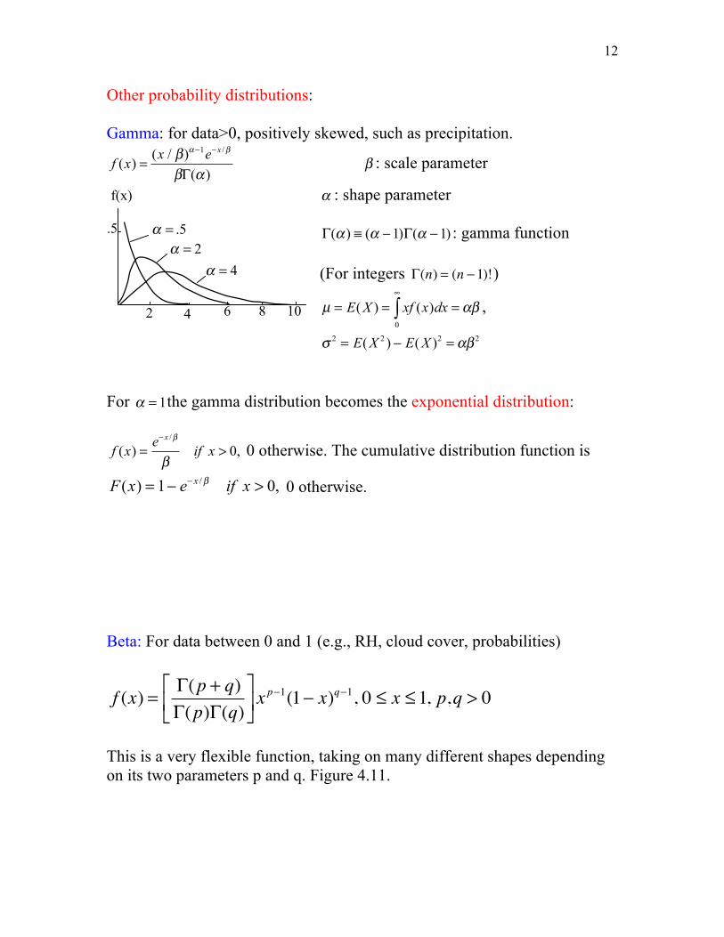
Other probability distributions: Gamma: for data>0, positively skewed, such as precipitation.

f (x) =

(x / β)α −1e− x /β

βΓ(α ) β : scale parameter

α : shape parameter

Γ(α ) ≡ (α −1)Γ(α −1) : gamma function (For integers Γ(n) = (n −1)!)

µ = E( X ) = xf (x)dx = αβ

0

∞

∫ ,

σ2 = E( X 2 ) − E( X )2 = αβ 2

For α = 1the gamma distribution becomes the exponential distribution:

f (x) =

e− x /β

βif x > 0, 0 otherwise. The cumulative distribution function is

F(x) = 1− e− x /β if x > 0, 0 otherwise. Beta: For data between 0 and 1 (e.g., RH, cloud cover, probabilities)

f (x) = Γ(p + q)Γ(p)Γ(q)

⎡

⎣⎢

⎤

⎦⎥ x

p−1(1− x)q−1, 0 ≤ x ≤ 1, p,q > 0

This is a very flexible function, taking on many different shapes depending on its two parameters p and q. Figure 4.11.

6 8 10

.52

2 4

f(x)

.5α = 2α =

4α =

13

µ = p / (p + q) ; σ2 =

pq(p + q)2 (p + q +1)

From these equations, the moment estimators (see parameter estimators) can be derived:

p̂ =x 2 (1− x )

s2− x; q̂ =

p̂(1− x )x

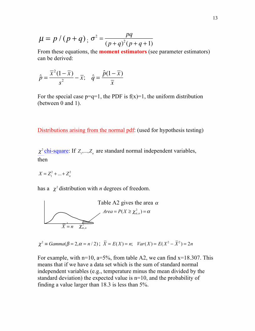
For the special case p=q=1, the PDF is f(x)=1, the uniform distribution (between 0 and 1). Distributions arising from the normal pdf: (used for hypothesis testing) χ

2 chi-square: If Z1,...,Zn are standard normal independent variables, then

X = Z12 + ...+ Zn

2 has a χ

2 distribution with n degrees of freedom. Table A2 gives the area α χ

2 ≡ Gamma(β = 2,α = n / 2) ; X = E( X ) = n; Var( X ) = E( X 2 − X 2 ) = 2n For example, with n=10, a=5%, from table A2, we can find x=18.307. This means that if we have a data set which is the sum of standard normal independent variables (e.g., temperature minus the mean divided by the standard deviation) the expected value is n=10, and the probability of finding a value larger than 18.3 is less than 5%.

X n=

2,nαχ

2,( )nArea P X αχ α= ≥ =

14

The exponential function is also the same as the chi-square for 2 degrees of freedom. For this reason it is appropriate for wind speed s = (u2 + v2 ) . An important application of the chi-square is to test goodness of fit: If you have a histogram with n bins, and a number of observations Oi and expected number of observations Ei (e.g., from a parametric distribution) in each bin, then the goodness of fit of the pdf to the data can be estimated using a chi-square test:

X 2 =(Oi − Ei )

2

Eii=1

n

∑ with n-1 degrees of freedom

The null hypothesis (that it is a good fit) is rejected at a 5% level of

significance if X 2 > χ(0.05,n−1)2

.

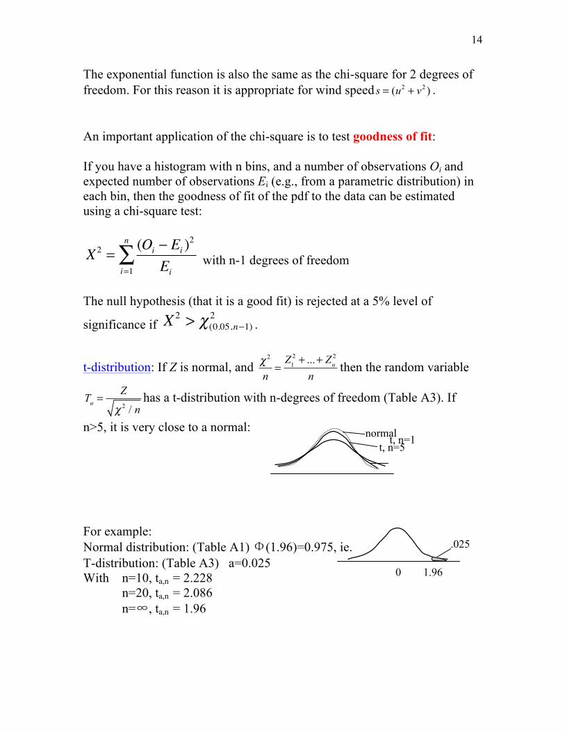
t-distribution: If Z is normal, and χ 2

n=

Z12 + ...+ Zn

2

nthen the random variable

Tn =

Z

χ 2 / nhas a t-distribution with n-degrees of freedom (Table A3). If

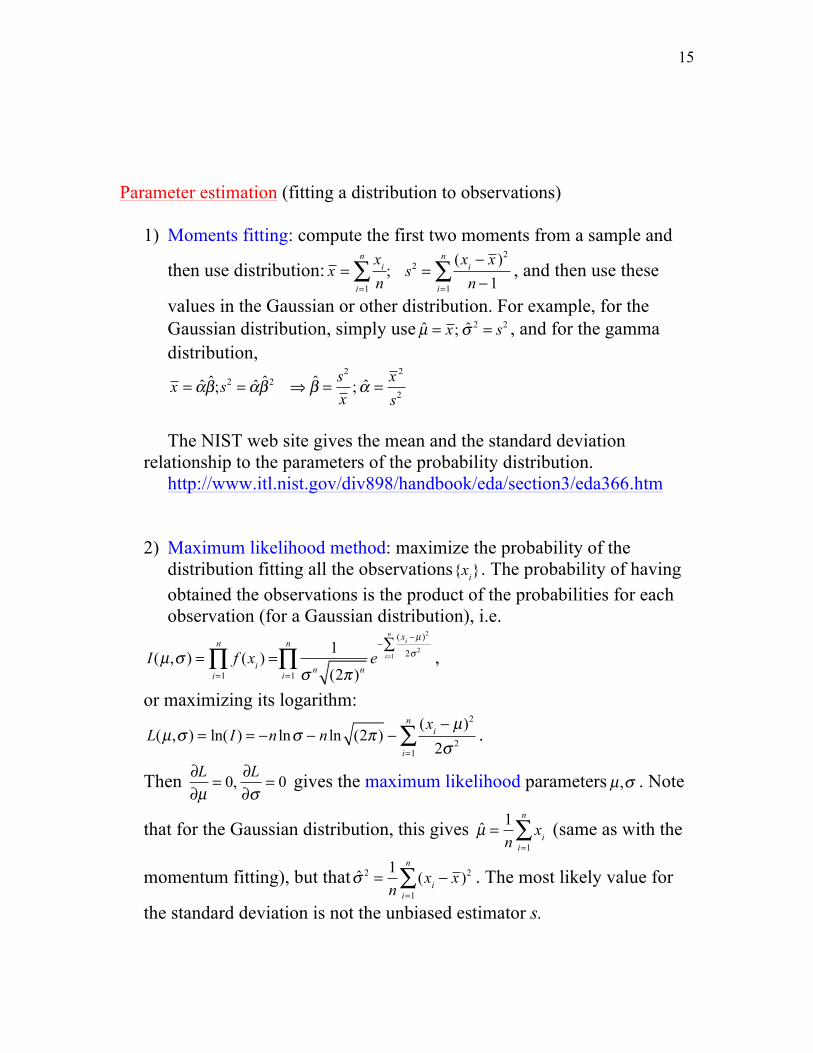
n>5, it is very close to a normal: For example: Normal distribution: (Table A1) Φ(1.96)=0.975, ie. T-distribution: (Table A3) a=0.025 With n=10, ta,n = 2.228

n=20, ta,n = 2.086 n=∞, ta,n = 1.96

normal t, n=5

t, n=1

.025

0 1.96

15

Parameter estimation (fitting a distribution to observations)

1) Moments fitting: compute the first two moments from a sample and

then use distribution: x =

xi

ni=1

n

∑ ; s2 =(xi − x )2

n −1i=1

n

∑ , and then use these

values in the Gaussian or other distribution. For example, for the Gaussian distribution, simply use µ̂ = x ; σ̂ 2 = s2 , and for the gamma distribution,

x = α̂β̂;s2 = α̂β̂ 2 ⇒ β̂ =

s2

x; α̂ =

x 2

s2

The NIST web site gives the mean and the standard deviation

relationship to the parameters of the probability distribution. http://www.itl.nist.gov/div898/handbook/eda/section3/eda366.htm

2) Maximum likelihood method: maximize the probability of the distribution fitting all the observations {xi}. The probability of having obtained the observations is the product of the probabilities for each observation (for a Gaussian distribution), i.e.

I(µ,σ ) = f (xi ) =

i=1

n

∏ 1

σ n (2π )ne−

( xi −µ )2

2σ 2i=1

n

∑

i=1

n

∏ ,

or maximizing its logarithm:

L(µ,σ ) = ln(I ) = −n lnσ − n ln (2π ) −

(xi − µ)2

2σ 2i=1

n

∑ .

Then

∂L∂µ

= 0,∂L∂σ

= 0 gives the maximum likelihood parameters µ,σ . Note

that for the Gaussian distribution, this gives µ̂ =

1n

xii=1

n

∑ (same as with the

momentum fitting), but that σ̂ 2 =

1n

(xi − x )2

i=1

n

∑ . The most likely value for

the standard deviation is not the unbiased estimator s.

16

Note: Likelihood is the probability distribution of the truth given a measurement. It is equal to the probability distribution of the measurement given the truth (Edwards, 1984). Goodness of fit Methods to test goodness of fit: a) Plot a PDF over the histogram and check how well it fits, (Fig 4.14) or b) check how well scatter plots of quantiles from the histogram

vs quantiles from the PDF fall onto the diagonal line (Fig 4.15)

1) A q-q plot is a plot of the quantiles of the first data set against the quantiles of the second data set. By a quantile, we mean the fraction (or percent) of points below the given value. That is, the 0.3 (or 30%) quantile is the point at which 30% percent of the data fall below and 70% fall above that value.

2) Both axes are in units of their respective data sets. That is, the actual quantile level is not plotted. If the data sets have the same size, the q-q plot is essentially a plot of sorted data set 1 against sorted data set 2.

c) Use the chi-square test (see above): X2 =

(Oi − Ei )2

Eii=1

n

∑

The fit is considered good (at a 5% level of significance) if X 2 < χ(0.05,n−1)

2

Extreme events: Gumbel distribution

17

Examples: coldest temperature in January, maximum daily precipitation in a summer, maximum river flow in the spring. Note that there are two time scales: a short scale (e.g., day) and a long scale: a number of years. Consider now the problem of obtaining the maximum (e.g., warmest temperature) extreme probability distribution:

CDF: F(x) = exp −exp −

x − ξβ

⎡

⎣⎢

⎤

⎦⎥

⎧⎨⎪

⎩⎪

⎫⎬⎪

⎭⎪: this can be derived from the

exponential distribution (von Storch and Zwiers, p49). The PDF can be obtained from the CDF:

PDF: f (x) =

1β

exp −exp −x − ξβ

⎡

⎣⎢

⎤

⎦⎥ −

x − ξβ

⎧⎨⎪

⎩⎪

⎫⎬⎪

⎭⎪

Parameter estimation for the maximum distribution

β̂ =

s 6π

; ξ̂ = x − γβ̂, γ = 0.57721... , Euler constant.

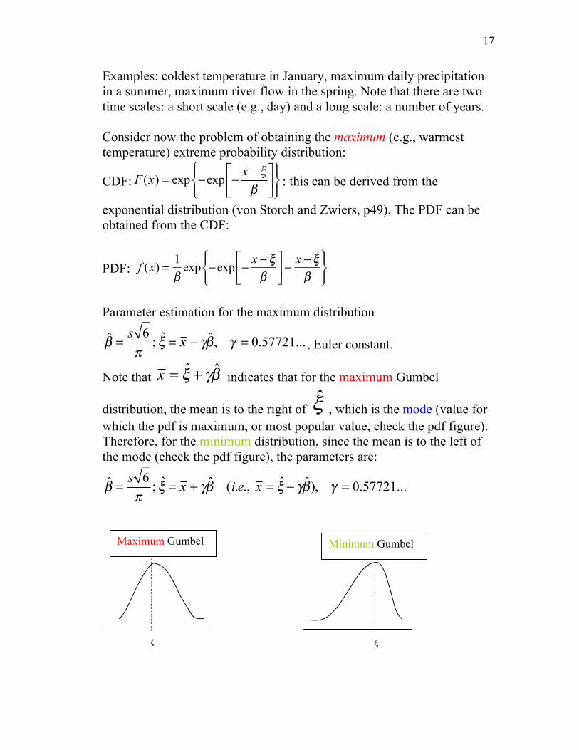
Note that x = ξ̂ + γβ̂ indicates that for the maximum Gumbel

distribution, the mean is to the right of ξ̂ , which is the mode (value for which the pdf is maximum, or most popular value, check the pdf figure). Therefore, for the minimum distribution, since the mean is to the left of the mode (check the pdf figure), the parameters are:

β̂ =

s 6π

; ξ̂ = x + γβ̂ (i.e., x = ξ̂ − γβ̂), γ = 0.57721...

ξ ξ

Maximum Gumbel Minimum Gumbel

18

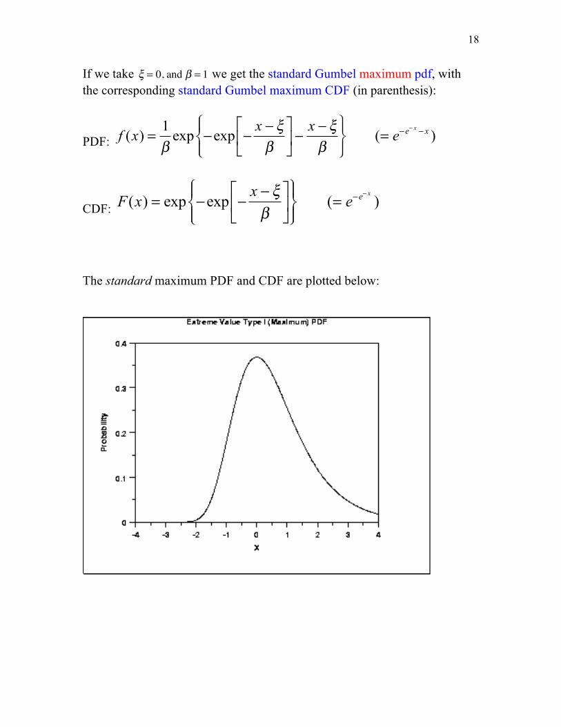
If we take ξ = 0, and β = 1 we get the standard Gumbel maximum pdf, with the corresponding standard Gumbel maximum CDF (in parenthesis):

PDF: f (x) =

1β

exp −exp −x − ξβ

⎡

⎣⎢

⎤

⎦⎥ −

x − ξβ

⎧⎨⎪

⎩⎪

⎫⎬⎪

⎭⎪(= e−e− x − x )

CDF: F(x) = exp −exp −

x − ξβ

⎡

⎣⎢

⎤

⎦⎥

⎧⎨⎪

⎩⎪

⎫⎬⎪

⎭⎪(= e−e− x

)

The standard maximum PDF and CDF are plotted below:

19

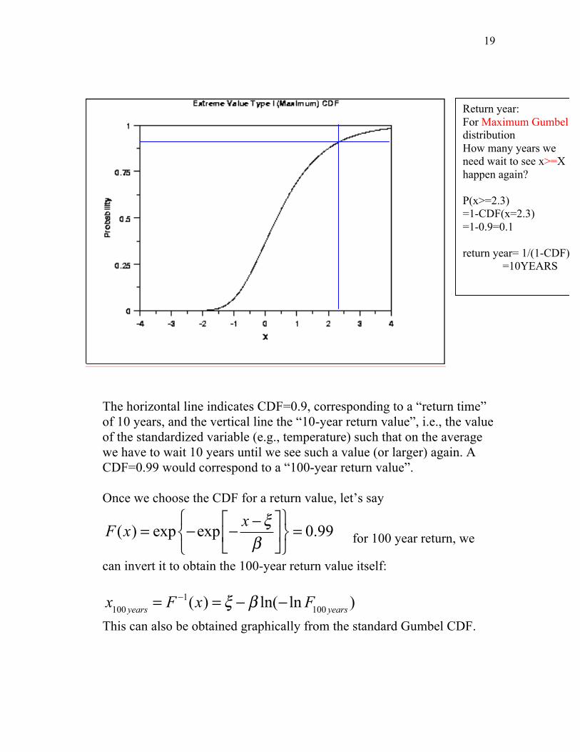
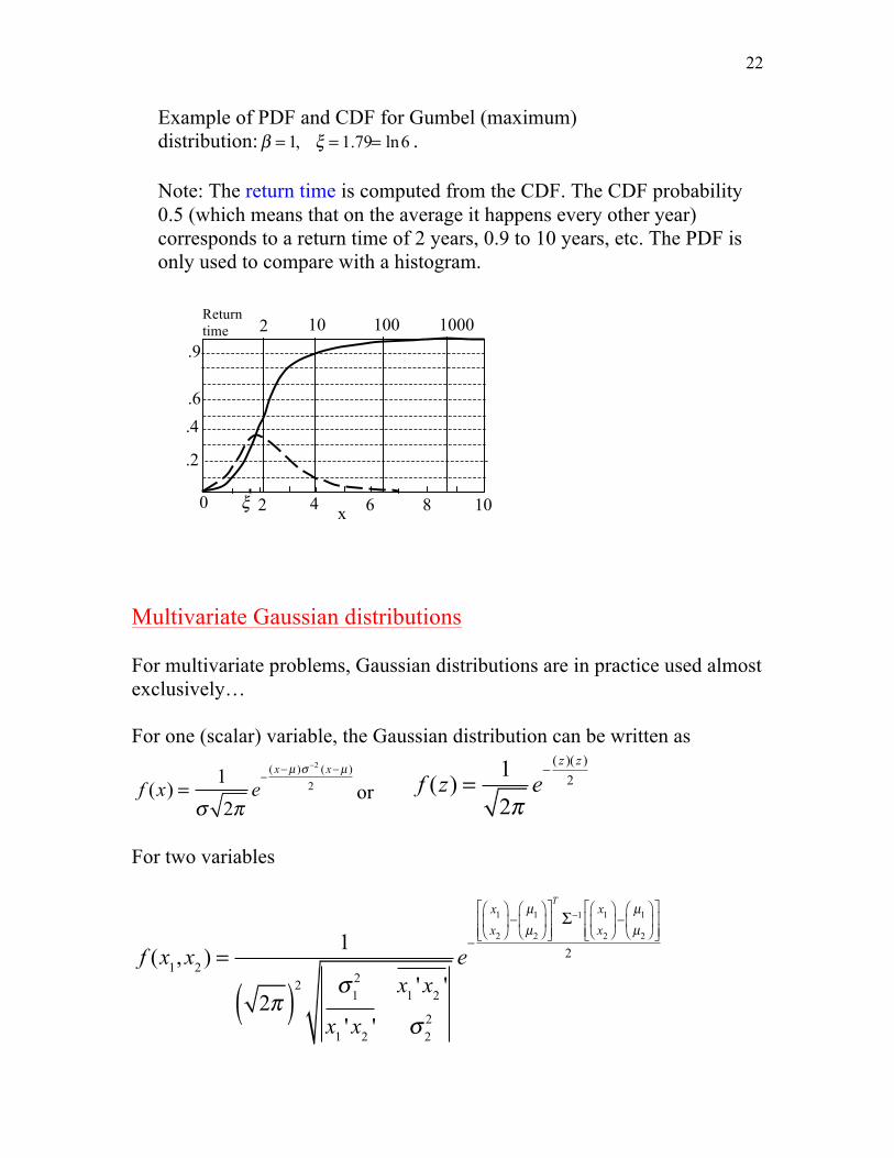
The horizontal line indicates CDF=0.9, corresponding to a “return time” of 10 years, and the vertical line the “10-year return value”, i.e., the value of the standardized variable (e.g., temperature) such that on the average we have to wait 10 years until we see such a value (or larger) again. A CDF=0.99 would correspond to a “100-year return value”. Once we choose the CDF for a return value, let’s say

F (x) = exp −exp − x −ξβ

⎡

⎣⎢

⎤

⎦⎥

⎧⎨⎩

⎫⎬⎭= 0.99 for 100 year return, we

can invert it to obtain the 100-year return value itself:

x100 years = F−1(x) = ξ − β ln(− lnF100 years )

This can also be obtained graphically from the standard Gumbel CDF.

Return year: For Maximum Gumbel distribution How many years we need wait to see x>=X happen again? P(x>=2.3) =1-CDF(x=2.3) =1-0.9=0.1 return year= 1/(1-CDF)

=10YEARS

20

If instead of looking for the maximum extreme event we are looking for the minimum (e.g., the coldest) extreme event, we have to reverse the

normalized x − ξβ to −

x − ξβ . The Gumbel minimum distributions

become (with the standard version in parenthesis)

PDF: f (x) =

1β

exp −expx − ξβ

⎡

⎣⎢

⎤

⎦⎥ +

x − ξβ

⎧⎨⎪

⎩⎪

⎫⎬⎪

⎭⎪(= e−ex + x )

The integral of e−ex + x is −e−ex

+ const = 1− e−ex

so that

CDF: F(x) = 1− exp −exp

x − ξβ

⎡

⎣⎢

⎤

⎦⎥

⎧⎨⎪

⎩⎪

⎫⎬⎪

⎭⎪(= 1− e−ex

)

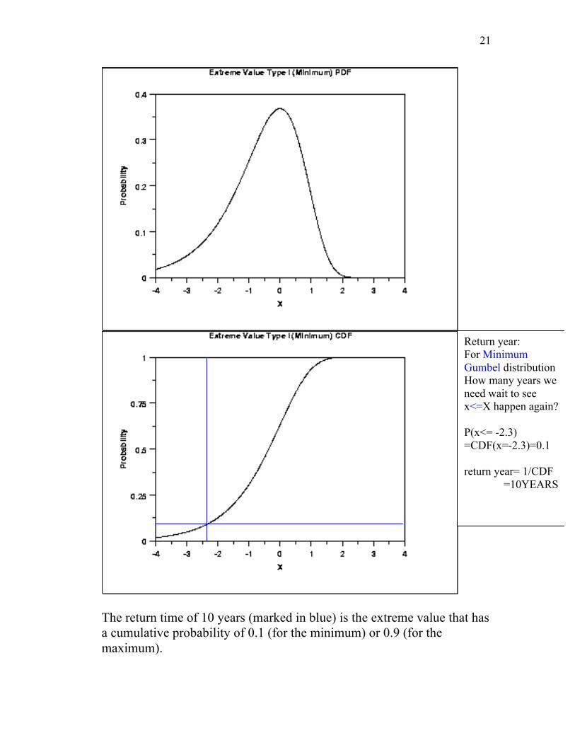
The PDF and CDF plots follow:

21

The return time of 10 years (marked in blue) is the extreme value that has a cumulative probability of 0.1 (for the minimum) or 0.9 (for the maximum).

Return year: For Minimum Gumbel distribution How many years we need wait to see x<=X happen again? P(x<= -2.3) =CDF(x=-2.3)=0.1 return year= 1/CDF

=10YEARS

22

Example of PDF and CDF for Gumbel (maximum) distribution: β = 1, ξ = 1.79= ln6 . Note: The return time is computed from the CDF. The CDF probability 0.5 (which means that on the average it happens every other year) corresponds to a return time of 2 years, 0.9 to 10 years, etc. The PDF is only used to compare with a histogram.

Multivariate Gaussian distributions For multivariate problems, Gaussian distributions are in practice used almost exclusively… For one (scalar) variable, the Gaussian distribution can be written as

f (x) =

1σ 2π

e−

( x−µ )σ−2 ( x−µ )2 or

f (z) =

12π

e−

( z )( z )2

For two variables

f (x1,x2 ) =1

2π( )2 σ12 x1 ' x2 '

x1 ' x2 ' σ 22

e−

x1

x2

⎛

⎝⎜

⎞

⎠⎟ −

µ1

µ2

⎛

⎝⎜

⎞

⎠⎟

⎡

⎣⎢⎢

⎤

⎦⎥⎥

T

Σ−1 x1

x2

⎛

⎝⎜

⎞

⎠⎟ −

µ1

µ2

⎛

⎝⎜

⎞

⎠⎟

⎡

⎣⎢⎢

⎤

⎦⎥⎥

2

2 4 6 8 10 0 x

10 100 1000 2 Return time

ξ

.2

.4 .6

.9

23

where

Σ =σ1

2 x1 ' x2 '

x1 ' x2 ' σ 22

⎡

⎣⎢⎢

⎤

⎦⎥⎥is the covariance matrix.

With two standardized variables

f (z1, z2 ) =1

2π( )2 1 ρρ 1

e−

z1

z2

⎛

⎝⎜

⎞

⎠⎟

⎡

⎣⎢⎢

⎤

⎦⎥⎥

T

R−1 z1

z2

⎛

⎝⎜

⎞

⎠⎟

⎡

⎣⎢⎢

⎤

⎦⎥⎥

2

where 11

Rρ

ρ⎡ ⎤

= ⎢ ⎥⎣ ⎦

is the correlation matrix.

For k variables, we define a vector

x =x1

...xk

⎛

⎝

⎜⎜⎜

⎞

⎠

⎟⎟⎟

and

f (x) =1

2π( )kΣ

e−

x−µ⎡⎣ ⎤⎦T Σ−1 x−µ⎡⎣ ⎤⎦

2.

For standardized variables,

f (z) =1

2π( )kR

e−

z⎡⎣ ⎤⎦T R−1 z⎡⎣ ⎤⎦

2where

Σ =σ1

2 ... x1 ' xk '... ... ...

x1 ' xk ' ... σ k2

⎡

⎣

⎢⎢⎢⎢

⎤

⎦

⎥⎥⎥⎥

and

R =1 ... ρ1k

... ... ...ρk1 ... 1

⎡

⎣

⎢⎢⎢

⎤

⎦

⎥⎥⎥

are the covariance and correlation matrices respectively. See figure 4.2/4.5 of Wilks showing a bivariate distribution.