Parameter Estimation of Mathematical Models Described by Differential Equations
32
Parameter Estimation of Mathematical Models Described by Differential Equations Hossein Zivaripiran Department of Computer Science University of Toronto Parameter Estimation – p.1/12
Transcript of Parameter Estimation of Mathematical Models Described by Differential Equations

Parameter Estimation of Mathematical Models Describedby Differential Equations
Hossein Zivaripiran
Department of Computer Science
University of Toronto
Parameter Estimation – p.1/12

Outline
� Modeling with Differential Equations (IVPs, DDEs)
� Modeling and Parameter Estimation
� Numerical Parameter Estimation of IVPs
� DDEs and Parameter Estimation
Parameter Estimation – p.2/12

Modeling with DE - Formulation
� An Initial Value Problem (IVP) for Ordinary Differential Equations (ODEs)
y′(t) = f(t, y(t))
y(t0) = y0
Parameter Estimation – p.3/12

Modeling with DE - Formulation
� An Initial Value Problem (IVP) for Ordinary Differential Equations (ODEs)
y′(t) = f(t, y(t))
y(t0) = y0
� Retarded Delay Differential Equations (RDDEs)
y′(t) = f(t, y(t), y(t− σ1), · · · , y(t− σν)) for t0 ≤ t ≤ tF
y(t) = φ(t), for t ≤ t0
σi = σi(t, y(t)) ≥ 0 delay (constant / time dependent / state dependent)
φ(t) history function (constant / time dependent)
� Neutral Delay Differential Equations (NDDEs)
y′(t) = f(t, y(t), y(t− σ1), · · · , y(t− σν),
y′(t− σν+1), · · · , y′(t− σν+ω)) for t0 ≤ t ≤ tF
y(t) = φ(t), y′(t) = φ′(t), for t ≤ t0,
Parameter Estimation – p.3/12
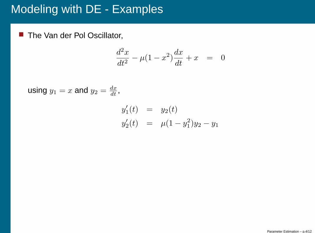
Modeling with DE - Examples
� The Van der Pol Oscillator,
d2x
dt2− µ(1− x2)
dx
dt+ x = 0
using y1 = x and y2 = dxdt
,
y′
1(t) = y2(t)
y′
2(t) = µ(1− y21)y2 − y1
Parameter Estimation – p.4/12
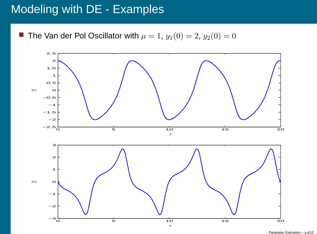
Modeling with DE - Examples
� The Van der Pol Oscillator with µ = 1, y1(0) = 2, y2(0) = 0
0 5 10 15 20−2.5
−2
−1.5
−1
−0.5
0
0.5
1
1.5
2
2.5
t
y1
0 5 10 15 20−3
−2
−1
0
1
2
3
t
y2
Parameter Estimation – p.4/12
Modeling with DE - Examples
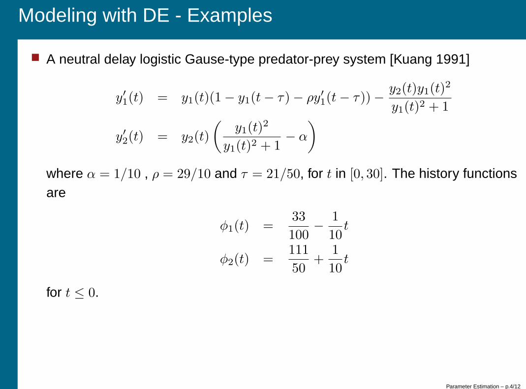
� A neutral delay logistic Gause-type predator-prey system [Kuang 1991]
y′
1(t) = y1(t)(1− y1(t− τ)− ρy′
1(t− τ))−y2(t)y1(t)
2
y1(t)2 + 1
y′
2(t) = y2(t)
(
y1(t)2
y1(t)2 + 1− α
)
where α = 1/10 , ρ = 29/10 and τ = 21/50, for t in [0, 30]. The history functionsare
φ1(t) =33
100−
1
10t
φ2(t) =111
50+
1
10t
for t ≤ 0.
Parameter Estimation – p.4/12
Modeling with DE - Examples
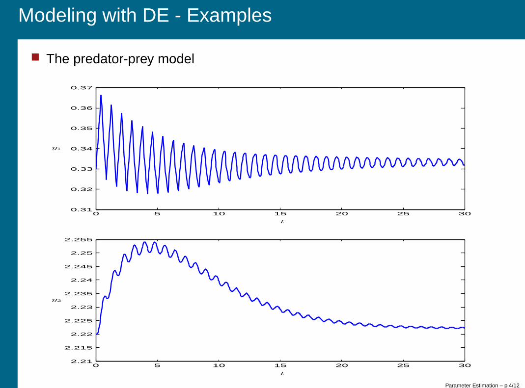
� The predator-prey model
0 5 10 15 20 25 300.31
0.32
0.33
0.34
0.35
0.36
0.37
t
y1
0 5 10 15 20 25 302.21
2.215
2.22
2.225
2.23
2.235
2.24
2.245
2.25
2.255
t
y2
Parameter Estimation – p.4/12

Modeling and Parameter Estimation - Definitions
� Parameterized Models
� A parameterized IVP
y′(t;p) = f(t, y(t;p);p)
y(t0) = y0(p)
For example p = [µ] in the Van der Pol oscillator
y′
1(t) = y2(t)
y′
2(t) = µ(1− y21)y2 − y1
� A simple parameterized DDE
y′(t;p) = f(t, y(t;p), y(t− σ(t;p));p) for t0(p) ≤ t
y(t;p) = φ(t;p), for t ≤ t0(p)
Parameter Estimation – p.5/12
Modeling and Parameter Estimation - Definitions
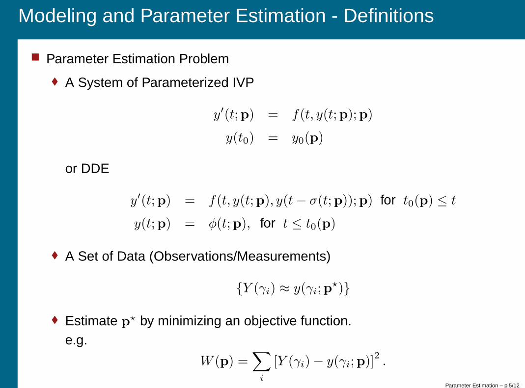
� Parameter Estimation Problem
� A System of Parameterized IVP
y′(t;p) = f(t, y(t;p);p)
y(t0) = y0(p)
or DDE
y′(t;p) = f(t, y(t;p), y(t− σ(t;p));p) for t0(p) ≤ t
y(t;p) = φ(t;p), for t ≤ t0(p)
� A Set of Data (Observations/Measurements)
{Y (γi) ≈ y(γi;p⋆)}
� Estimate p⋆ by minimizing an objective function.
e.g.
W (p) =∑
i
[Y (γi)− y(γi;p)]2.
Parameter Estimation – p.5/12
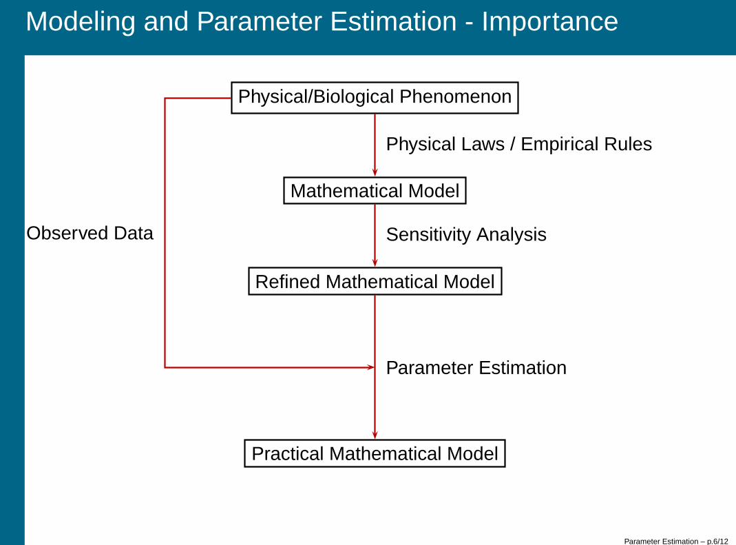
Modeling and Parameter Estimation - Importance
Physical/Biological Phenomenon
Mathematical Model
Refined Mathematical Model
Practical Mathematical Model
Physical Laws / Empirical Rules
Sensitivity Analysis
Parameter Estimation
Observed Data
Parameter Estimation – p.6/12

Modeling and Parameter Estimation - Optimizers
� Algorithms for Nonlinear Least-Squares� Unconstrained
minp
W (p) =∑
i
[Y (γi) − y(γi;p)]2 .
↓
Levenberg-MarquardtVariations of Sequential Quadratic Programming (SQP)
� Constrained
minp
W (p) =∑
i
[Y (γi) − y(γi;p)]2 ,
cj(p) = 0, j ∈ E,
cj(p) ≥ 0, j ∈ I.
↓
Sequential Quadratic Programming (SQP)
Parameter Estimation – p.7/12

Numerical Parameter Estimation of IVPs
The initial value approach :
1. Choose an initial guess for the parameters
2. Solve model equations
3. Check optimality conditions, (if satisfied ⇒ stop).
4. Choose a better value for the parameters and continue with (2)
The main difficulty : If the parameters are far from the correct ones the trial trajectory soonloses contact to the measurements.
If the optimization method needs to compute the gradient or the Hessian of the objectivefunction,
(
∂W (p)
∂pl
)
= −2∑
i
[Y (γi) − y(γi;p)]
(
∂y(γi;p)
∂pl
)
(
∂2W (p)
∂pl∂pm
)
= 2∑
i
[(
∂y(γi;p)
∂pl
) (
∂y(γi;p)
∂pm
)
− [Y (γi) − y(γi;p)]
(
∂2y(γi;p)
∂pl∂pm
)]
the sensitivity equations are usually used to provide the required values. An alternativeapproach is to use a divided-difference approximation.
Parameter Estimation – p.8/12
Numerical Parameter Estimation of IVPs
� A Simple Example,
� The IVP
y′
1(t) = ay2(t)
y′
2(t) = −ay1(t)
� with initial conditions
y1(0) = 0
y2(0) = 1
� the analytical solution is
y1(t) = sin(at)
y2(t) = cos(at)
Parameter Estimation – p.8/12

Numerical Parameter Estimation of IVPs
0 1 2 3 4 5 6 7−1
−0.8
−0.6
−0.4
−0.2
0
0.2
0.4
0.6
0.8
1
t
y 1(t
)
a*=1a=1.05a=1.1a=1.15a=1.45a=1.5a=1.55
Parameter Estimation – p.8/12

Numerical Parameter Estimation of IVPs
0 0.5 1 1.5 20
0.5
1
1.5
2
2.5
3
a
W(a
)
Parameter Estimation – p.8/12

Numerical Parameter Estimation of IVPs
Multiple shooting :
� Partitions the fitting interval into many subintervals, each having its own initial values.
� The measurements are used to get starting guesses for initial values of each interval.
� In an iterative process, the algorithm minimizes W (p) on the one hand and enforces thecontinuity of the full trajectory on the other hand.
Advantages: Divergences are avoided and the danger of local minima is reduced.
Parameter Estimation – p.8/12

Numerical Parameter Estimation of IVPs
0 1 2 3 4 5 6 7−1
−0.8
−0.6
−0.4
−0.2
0
0.2
0.4
0.6
0.8
1
t
y 1(t
)
Parameter Estimation – p.8/12
DDEs and Parameter Estimation
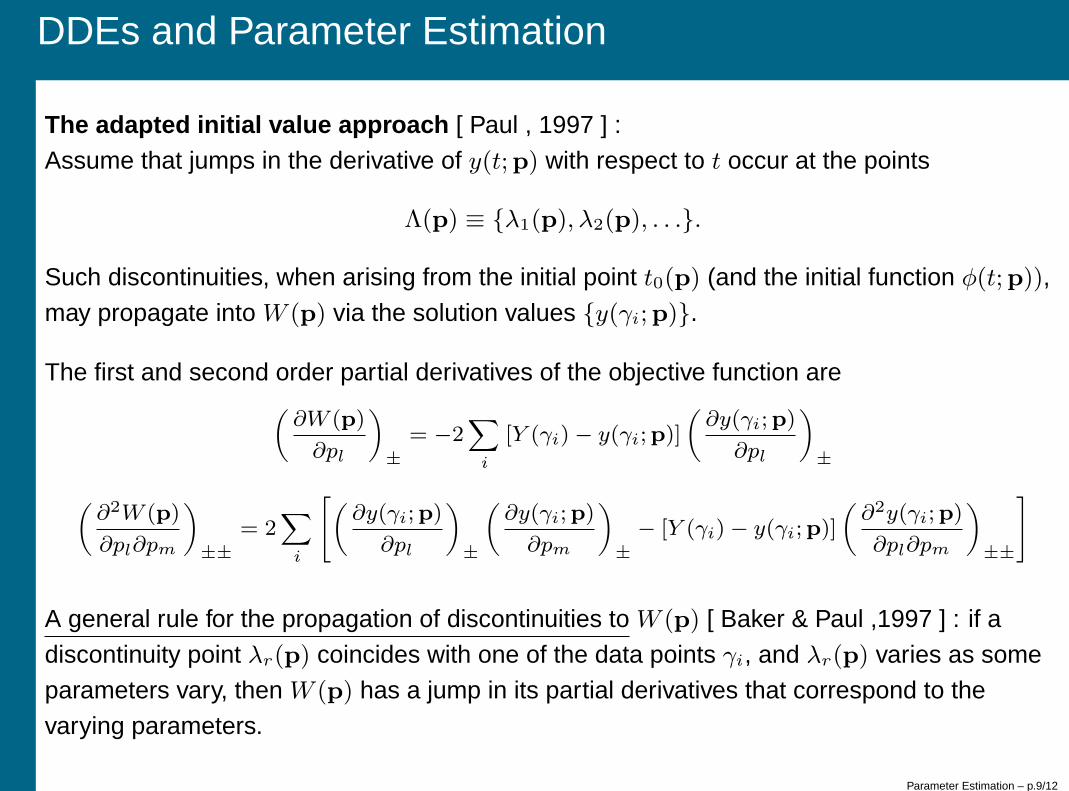
The adapted initial value approach [ Paul , 1997 ] :Assume that jumps in the derivative of y(t;p) with respect to t occur at the points
Λ(p) ≡ {λ1(p), λ2(p), . . .}.
Such discontinuities, when arising from the initial point t0(p) (and the initial function φ(t;p)),may propagate into W (p) via the solution values {y(γi;p)}.
The first and second order partial derivatives of the objective function are(
∂W (p)
∂pl
)
±
= −2∑
i
[Y (γi) − y(γi;p)]
(
∂y(γi;p)
∂pl
)
±
(
∂2W (p)
∂pl∂pm
)
±±
= 2∑
i
[
(
∂y(γi;p)
∂pl
)
±
(
∂y(γi;p)
∂pm
)
±
− [Y (γi) − y(γi;p)]
(
∂2y(γi;p)
∂pl∂pm
)
±±
]
A general rule for the propagation of discontinuities to W (p) [ Baker & Paul ,1997 ] : if adiscontinuity point λr(p) coincides with one of the data points γi, and λr(p) varies as someparameters vary, then W (p) has a jump in its partial derivatives that correspond to thevarying parameters.
Parameter Estimation – p.9/12

DDEs and Parameter Estimation
Multiple shooting [ Horbet et al., 2002 ] :
Use cubic splines to parameterize the initial curves and formulate the continuity of thetrajectory in terms of these spline variables.
A two-phase procedure:
� During the first iterations of the optimization, the spline variables are held fixed becausethey are expected to be estimated well from the data.
� After the algorithm has converged for the first time, they are released and fitted togetherwith the other variables until the final convergence is achieved.
Can attain higher convergence rate in the case of noisy data.
Parameter Estimation – p.9/12

DDEs and Parameter Estimation
The full discretization approach [ Murphy, 1990 ]:
Use linear splines to describe solution and delay functions.
As the result the problem becomes a very large minimization problem.
The number of mesh points is increased gradually to be able to satisfy the specified errortolerance.
Although the method has the generality of dealing with any kinds of unknown parameters, itsuffers from the heavy computations, slow convergence rate and possibility of being trappedin a local minimum.
Parameter Estimation – p.9/12
DDEs and Parameter Estimation
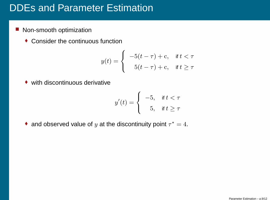
� Non-smooth optimization
� Consider the continuous function
y(t) =
−5(t − τ) + c, if t < τ
5(t − τ) + c, if t ≥ τ
� with discontinuous derivative
y′(t) =
−5, if t < τ
5, if t ≥ τ
� and observed value of y at the discontinuity point τ⋆ = 4.
Parameter Estimation – p.9/12

DDEs and Parameter Estimation
0 1 2 3 4 5 6 70
5
10
15
20
25
tτ
y(t
)
c
Parameter Estimation – p.9/12

DDEs and Parameter Estimation
3 3.5 4 4.5 5−60
−40
−20
0
20
40
60
τ
W(τ )
∂W(τ )
∂τ
Parameter Estimation – p.9/12

DDEs and Parameter Estimation
� Try to find τ⋆ using MATLAB’s unconstrained minimization routine fminunc
⇓
31 iterations .
� Try to use MATLAB’s constrained minimization routine fminconwith the added constraint
τ ≤ 4
⇓
2 iterations .
� Try to use MATLAB’s constrained minimization routine fminconwith the added constraint
τ ≥ 4
⇓
2 iterations .
Parameter Estimation – p.9/12
DDEs and Parameter Estimation - Safe Minimization
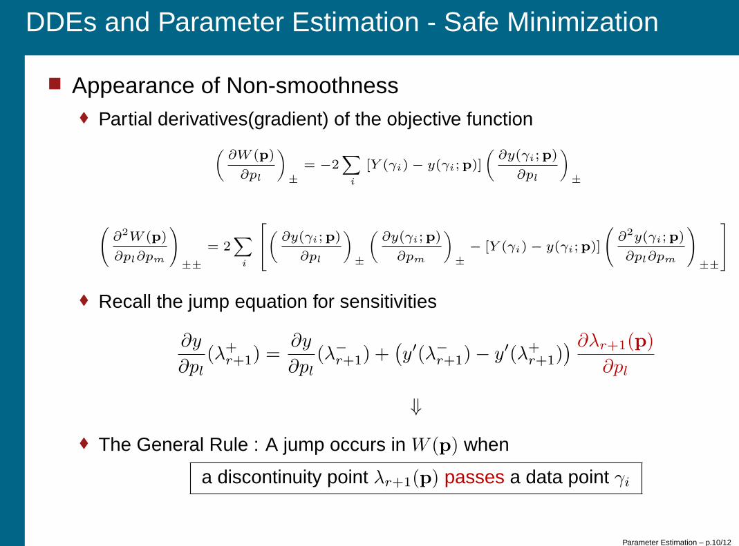
� Appearance of Non-smoothness� Partial derivatives(gradient) of the objective function
(
∂W (p)
∂pl
)
±
= −2∑
i
[Y (γi) − y(γi;p)]
(
∂y(γi;p)
∂pl
)
±
(
∂2W (p)
∂pl∂pm
)
±±
= 2∑
i
(
∂y(γi;p)
∂pl
)
±
(
∂y(γi;p)
∂pm
)
±
− [Y (γi) − y(γi;p)]
(
∂2y(γi;p)
∂pl∂pm
)
±±
� Recall the jump equation for sensitivities
∂y
∂pl
(λ+r+1) =
∂y
∂pl
(λ−
r+1) +(
y′(λ−
r+1)− y′(λ+r+1)
) ∂λr+1(p)
∂pl
⇓
� The General Rule : A jump occurs in W (p) when
a discontinuity point λr+1(p) passes a data point γi
Parameter Estimation – p.10/12
DDEs and Parameter Estimation - Safe Minimization
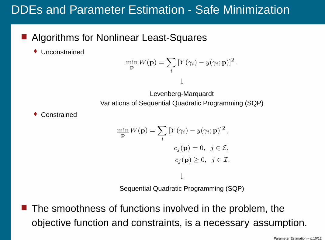
� Algorithms for Nonlinear Least-Squares� Unconstrained
minp
W (p) =∑
i
[Y (γi) − y(γi;p)]2 .
↓
Levenberg-MarquardtVariations of Sequential Quadratic Programming (SQP)
� Constrained
minp
W (p) =∑
i
[Y (γi) − y(γi;p)]2 ,
cj(p) = 0, j ∈ E,
cj(p) ≥ 0, j ∈ I.
↓
Sequential Quadratic Programming (SQP)
� The smoothness of functions involved in the problem, theobjective function and constraints, is a necessary assumption.
Parameter Estimation – p.10/12

DDEs and Parameter Estimation - Safe Minimization
� Avoiding The Non-smoothness
t
y
λr(p) γi λr+1(p)
t
y
λr(p)
γi
λr+1(p)
true solutioncontiniously extended solutiondiscontinuity pointdata point
Force the ordering by adding λr(p) ≤ γi ≤ λr+1(p) to the set of constraints.
The partial derivatives (gradient) of the new constraints ,∂λr+1(p)
∂p, can be computed recursively.
Parameter Estimation – p.10/12
DDEs and Parameter Estimation - Safe Minimization
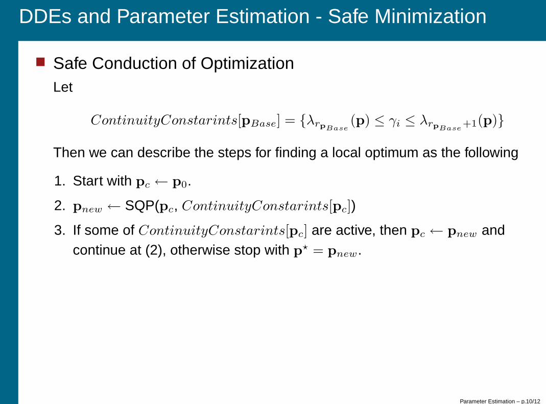
� Safe Conduction of OptimizationLet
ContinuityConstarints[pBase] = {λrpBase(p) ≤ γi ≤ λrpBase
+1(p)}
Then we can describe the steps for finding a local optimum as the following
1. Start with pc ← p0.
2. pnew ← SQP(pc, ContinuityConstarints[pc])
3. If some of ContinuityConstarints[pc] are active, then pc ← pnew andcontinue at (2), otherwise stop with p
⋆ = pnew.
Parameter Estimation – p.10/12

DDEs and Parameter Estimation - A Test Case
� Estimating τ for the predator-prey model
y′1(t) = y1(t)(1 − y1(t − τ) − ρy′
1(t − τ)) −y2(t)y1(t)2
y1(t)2 + 1
y′2(t) = y2(t)
(
y1(t)2
y1(t)2 + 1− α
)
� Start with up to 10% random perturbation in original τ ,and up to 3% randomly perturbed y(t; τ) as Data (Y ).For γ’s we choose 10 random points, one of which is a discontinuity point.
� Run the parameter estimator 3 times.
� Results
Estimator Choice FCN OBJ
Very Simple 72,2697 0.000142917
Using Sensitivities 26,942 0.000142917
Adding Constraints 9,916 0.000142917
Parameter Estimation – p.11/12
DDEs and Parameter Estimation - The Role of Data
Back to First Talk!
Parameter Estimation – p.12/12