Parallel Programming for Graph Analysis
76
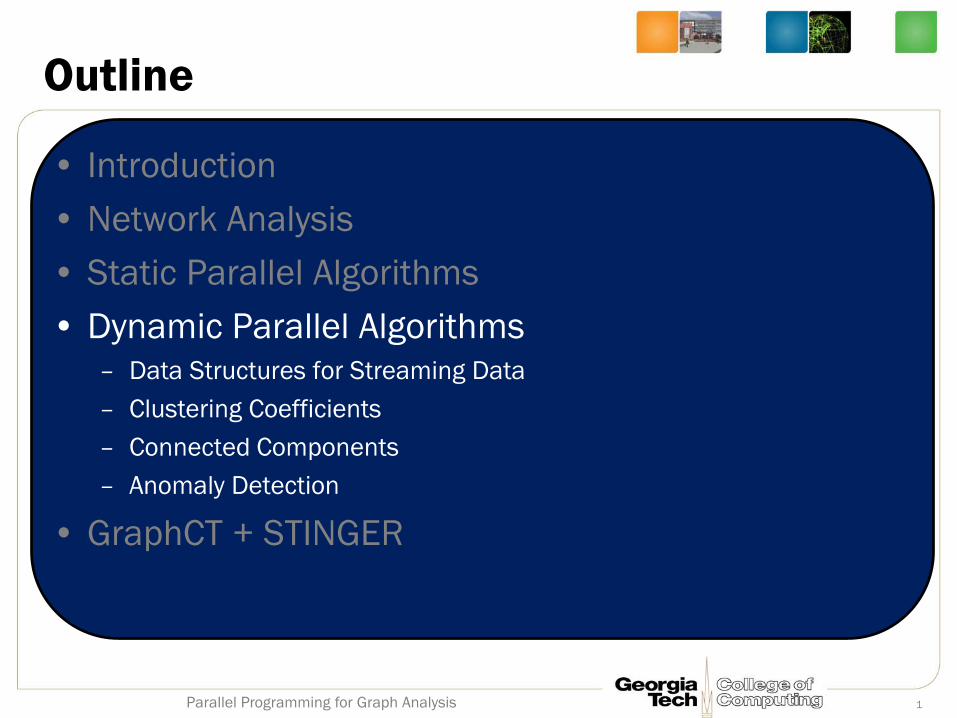
Outline • Introduction • Network Analysis • Static Parallel Algorithms • Dynamic Parallel Algorithms – Data Structures for Streaming Data – Clustering Coefficients – Connected Components – Anomaly Detection • GraphCT + STINGER Parallel Programming for Graph Analysis 1
Transcript of Parallel Programming for Graph Analysis
Outline
• Introduction
• Network Analysis
• Static Parallel Algorithms
• Dynamic Parallel Algorithms – Data Structures for Streaming Data
– Clustering Coefficients
– Connected Components
– Anomaly Detection
• GraphCT + STINGER
Parallel Programming for Graph Analysis 1

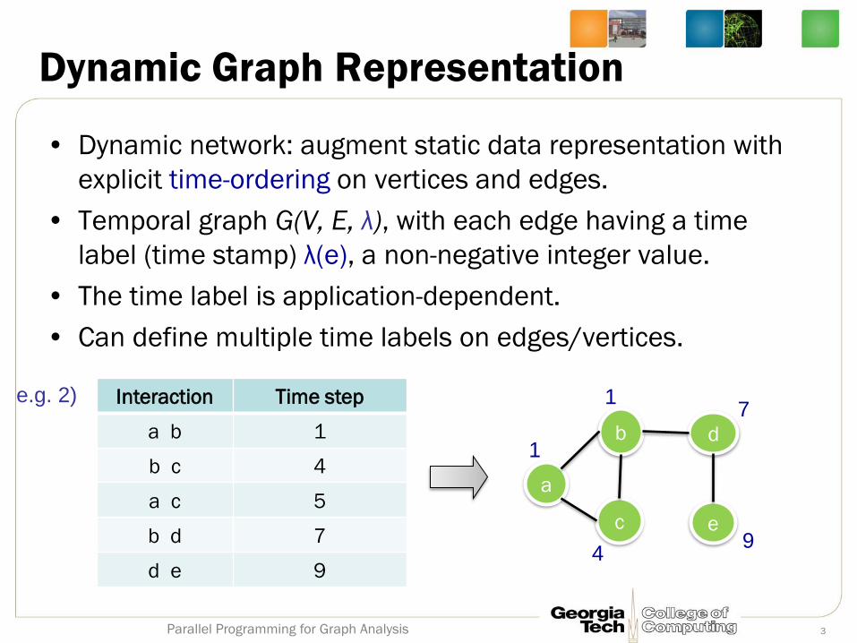
Dynamic Graph Representation
• Dynamic network: augment static data representation with
explicit time-ordering on vertices and edges.
• Temporal graph G(V, E, λ), with each edge having a time
label (time stamp) λ(e), a non-negative integer value.
• The time label is application-dependent.
• Can define multiple time labels on edges/vertices.
2
a
b
c
d
e
1
5
9 4
Interaction Time step
a b 1
b c 4
a c 5
b d 7
d e 9
e.g. 1) 7
Parallel Programming for Graph Analysis
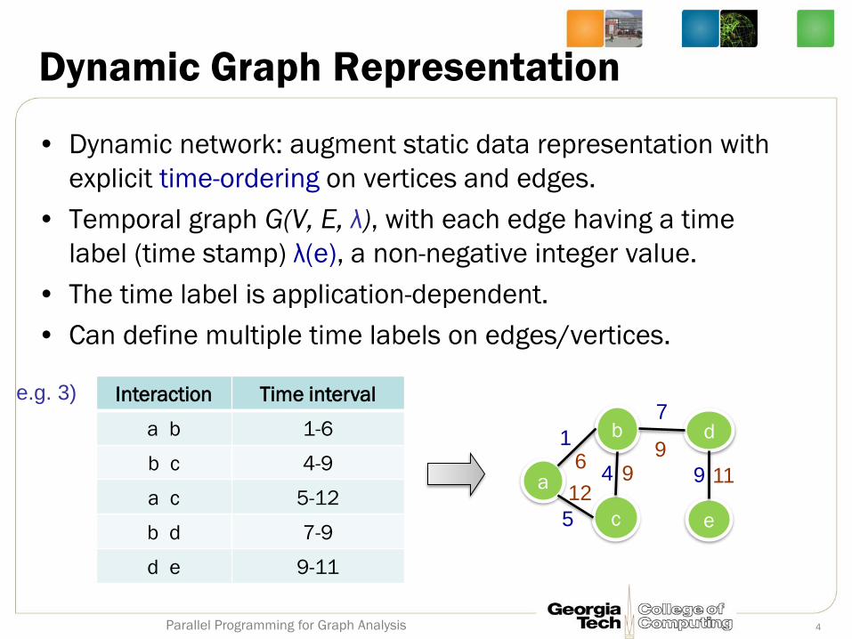
Dynamic Graph Representation
• Dynamic network: augment static data representation with
explicit time-ordering on vertices and edges.
• Temporal graph G(V, E, λ), with each edge having a time
label (time stamp) λ(e), a non-negative integer value.
• The time label is application-dependent.
• Can define multiple time labels on edges/vertices.
3
a
b
c
d
e
1
9 4
Interaction Time step
a b 1
b c 4
a c 5
b d 7
d e 9
e.g. 2) 1 7
Parallel Programming for Graph Analysis
Dynamic Graph Representation
Parallel Programming for Graph Analysis 4
• Dynamic network: augment static data representation with
explicit time-ordering on vertices and edges.
• Temporal graph G(V, E, λ), with each edge having a time
label (time stamp) λ(e), a non-negative integer value.
• The time label is application-dependent.
• Can define multiple time labels on edges/vertices.
a
b
c
d
e
1
5
9 4
Interaction Time interval
a b 1-6
b c 4-9
a c 5-12
b d 7-9
d e 9-11
e.g. 3) 7
6 9
12
9
11
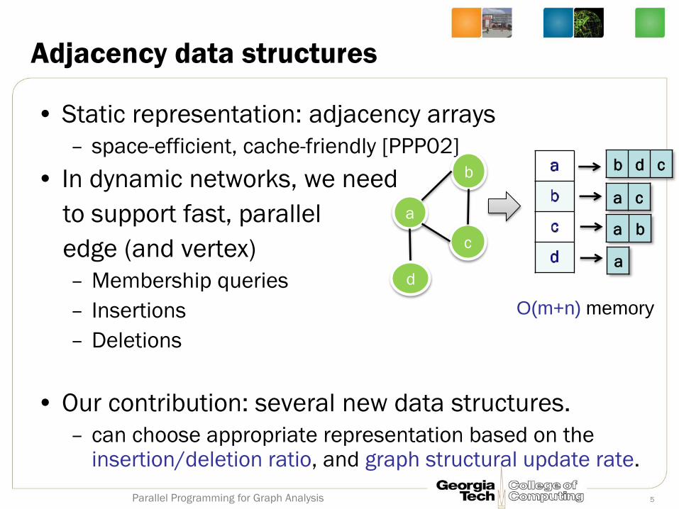
Adjacency data structures
• Static representation: adjacency arrays
– space-efficient, cache-friendly [PPP02]
• In dynamic networks, we need
to support fast, parallel
edge (and vertex)
– Membership queries
– Insertions
– Deletions
• Our contribution: several new data structures.
– can choose appropriate representation based on the insertion/deletion ratio, and graph structural update rate.
a
b
c
d
a b
b d c
a
a c
O(m+n) memory
5 Parallel Programming for Graph Analysis
p
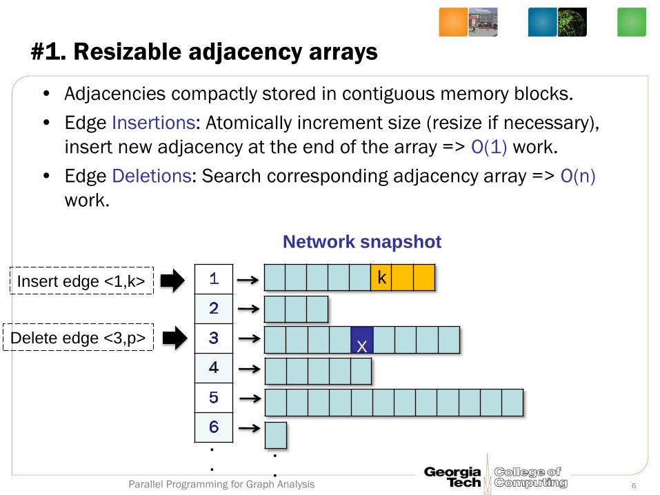
#1. Resizable adjacency arrays
• Adjacencies compactly stored in contiguous memory blocks.
• Edge Insertions: Atomically increment size (resize if necessary),
insert new adjacency at the end of the array => O(1) work.
• Edge Deletions: Search corresponding adjacency array => O(n)
work.
Insert edge <1,k>
Delete edge <3,p> X
Network snapshot
.
. .
.
k
6 Parallel Programming for Graph Analysis
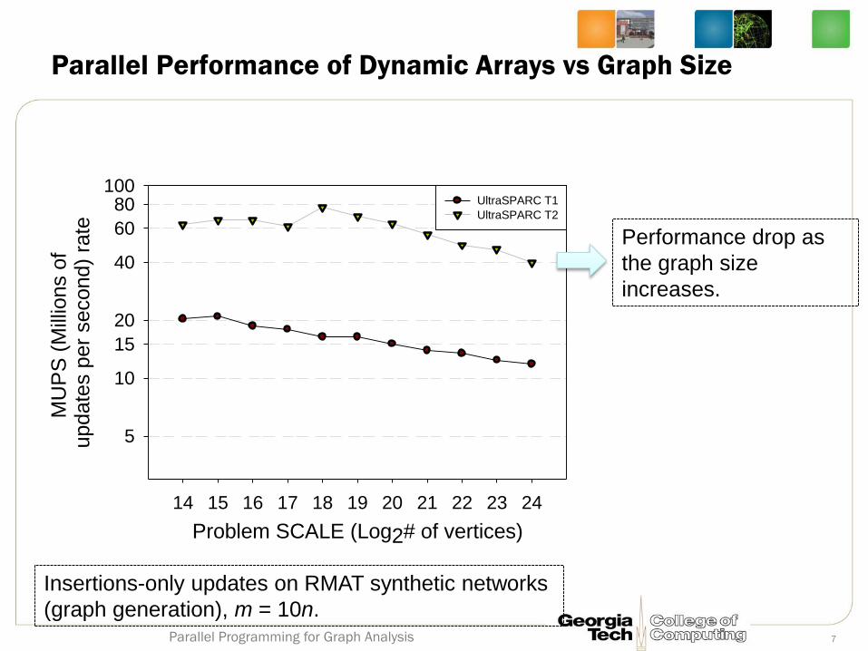
Parallel Performance of Dynamic Arrays vs Graph Size
Problem SCALE (Log2# of vertices)
14 15 16 17 18 19 20 21 22 23 24
MU
PS
(M
illio
ns o
f update
s p
er
second)
rate
5
10
15
20
40
60
80100
UltraSPARC T1
UltraSPARC T2
Insertions-only updates on RMAT synthetic networks
(graph generation), m = 10n.
Performance drop as
the graph size
increases.
7 Parallel Programming for Graph Analysis
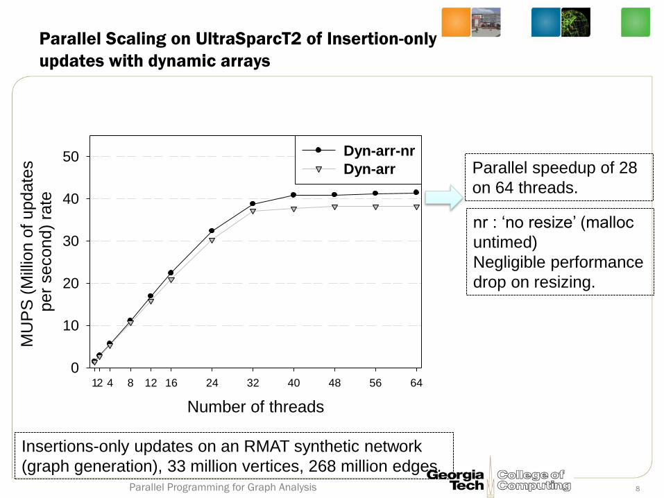
Parallel Scaling on UltraSparcT2 of Insertion-only
updates with dynamic arrays
Insertions-only updates on an RMAT synthetic network
(graph generation), 33 million vertices, 268 million edges.
nr : ‘no resize’ (malloc
untimed)
Negligible performance
drop on resizing.
Number of threads
12 4 8 12 16 24 32 40 48 56 64
MU
PS
(M
illio
n o
f update
s
per
second)
rate
0
10
20
30
40
50 Dyn-arr-nr
Dyn-arr Parallel speedup of 28
on 64 threads.
8 Parallel Programming for Graph Analysis

• [SA96] Binary search trees with priorities associated with each node, and
maintained in heap order.
• Self-balancing tree structure. O(log n) search, insertion, and deletion.
• Existing work-efficient parallel algorithms for set operations (union,
intersection, difference) on treaps.
• Our contribution: parallelization of treap operations
#2. Treaps
1 Adjacencies of
a vertex
represented
as a treap: 2 3
7 4 5
9 8 6
1
7
8
13
20
18
16
9
12
Vertex ID
Priority (random integer)
9 Parallel Programming for Graph Analysis
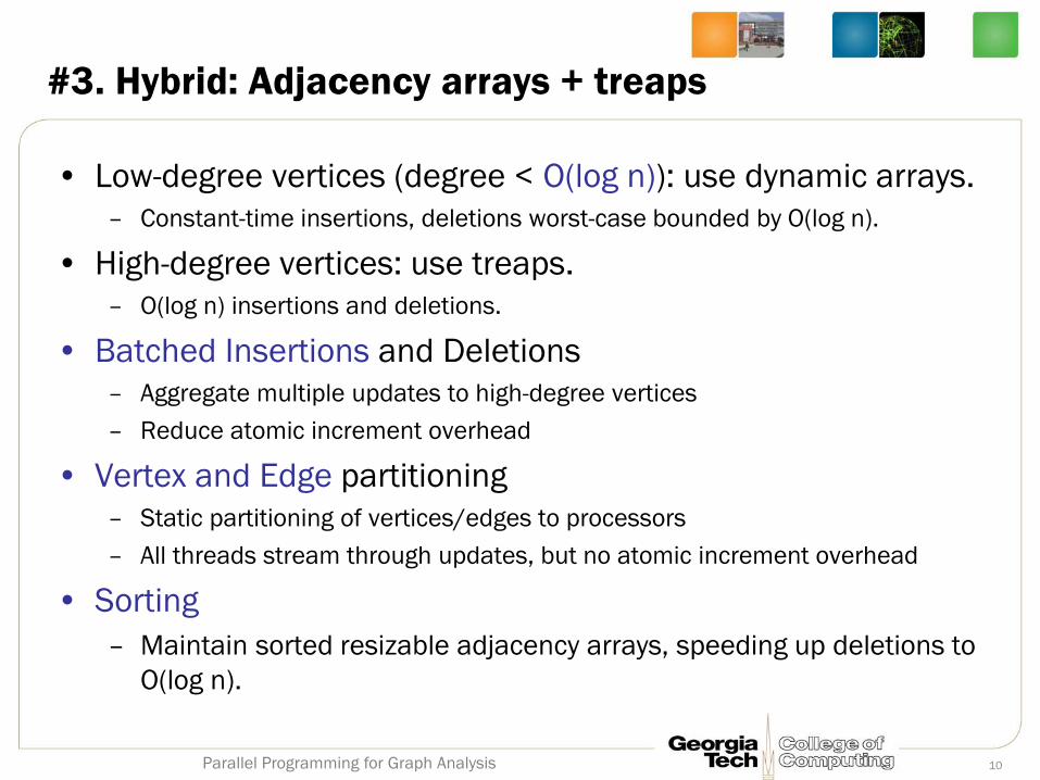
• Low-degree vertices (degree < O(log n)): use dynamic arrays.
– Constant-time insertions, deletions worst-case bounded by O(log n).
• High-degree vertices: use treaps.
– O(log n) insertions and deletions.
• Batched Insertions and Deletions
– Aggregate multiple updates to high-degree vertices
– Reduce atomic increment overhead
• Vertex and Edge partitioning
– Static partitioning of vertices/edges to processors
– All threads stream through updates, but no atomic increment overhead
• Sorting
– Maintain sorted resizable adjacency arrays, speeding up deletions to
O(log n).
#3. Hybrid: Adjacency arrays + treaps
10 Parallel Programming for Graph Analysis
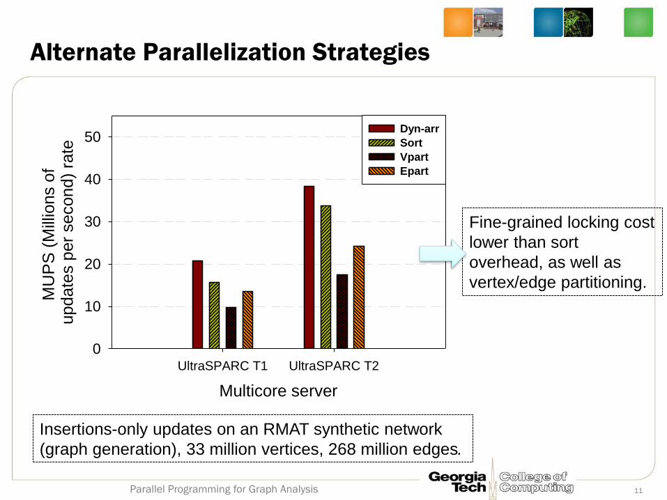
Alternate Parallelization Strategies
Multicore server
UltraSPARC T1 UltraSPARC T2
MU
PS
(M
illio
ns o
f update
s p
er
second)
rate
0
10
20
30
40
50Dyn-arr
Sort
Vpart
Epart
Insertions-only updates on an RMAT synthetic network
(graph generation), 33 million vertices, 268 million edges.
Fine-grained locking cost
lower than sort
overhead, as well as
vertex/edge partitioning.
11 Parallel Programming for Graph Analysis
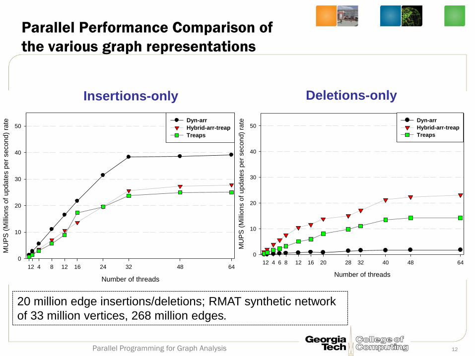
Parallel Performance Comparison of
the various graph representations
Number of threads
12 4 8 12 16 24 32 48 64
MU
PS
(M
illio
ns o
f u
pd
ate
s p
er
se
co
nd
) ra
te
0
10
20
30
40
50Dyn-arr
Hybrid-arr-treap
Treaps
Number of threads
12 4 6 8 12 16 20 28 32 40 48 64
MU
PS
(M
illio
ns o
f u
pd
ate
s p
er
se
co
nd
) ra
te
0
10
20
30
40
50Dyn-arr
Hybrid-arr-treap
Treaps
20 million edge insertions/deletions; RMAT synthetic network
of 33 million vertices, 268 million edges.
Insertions-only Deletions-only
12 Parallel Programming for Graph Analysis
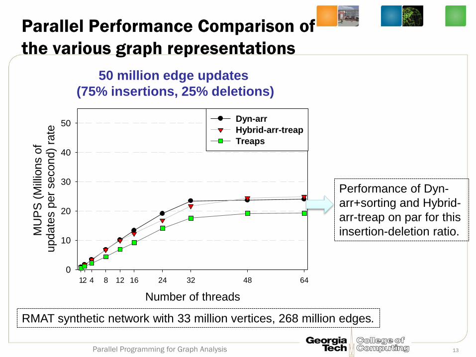
Parallel Performance Comparison of
the various graph representations
Number of threads
12 4 8 12 16 24 32 48 64
MU
PS
(M
illio
ns o
f update
s p
er
second)
rate
0
10
20
30
40
50Dyn-arr
Hybrid-arr-treap
Treaps
RMAT synthetic network with 33 million vertices, 268 million edges.
50 million edge updates
(75% insertions, 25% deletions)
Performance of Dyn-
arr+sorting and Hybrid-
arr-treap on par for this
insertion-deletion ratio.
13 Parallel Programming for Graph Analysis
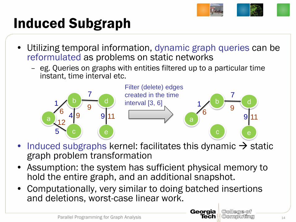
• Utilizing temporal information, dynamic graph queries can be reformulated as problems on static networks – eg. Queries on graphs with entities filtered up to a particular time
instant, time interval etc.
• Induced subgraphs kernel: facilitates this dynamic static graph problem transformation
• Assumption: the system has sufficient physical memory to hold the entire graph, and an additional snapshot.
• Computationally, very similar to doing batched insertions and deletions, worst-case linear work.
Induced Subgraph
a
b
c
d
e
1
5
9 4
7
6 9
12
9
11
Filter (delete) edges
created in the time
interval [3, 6]
a
b d
e
1
9
7
6 9
11
c
14 Parallel Programming for Graph Analysis
• Level-synchronous graph traversal for low-diameter
graphs, and each edge in the graph visited only
once/twice.
• Dynamic networks
– Filter vertices and edges according to time-stamp
information, recompute BFS from scratch
– Dynamic graph algorithms for BFS [DFR06]: better
amortized work bounds, space requirements – harder to
parallelize.
• Our contribution: Fast, lock-free parallel algorithm
for shared memory parallel systems processing
time stamps, and with edge filtering
Graph traversal
15 Parallel Programming for Graph Analysis
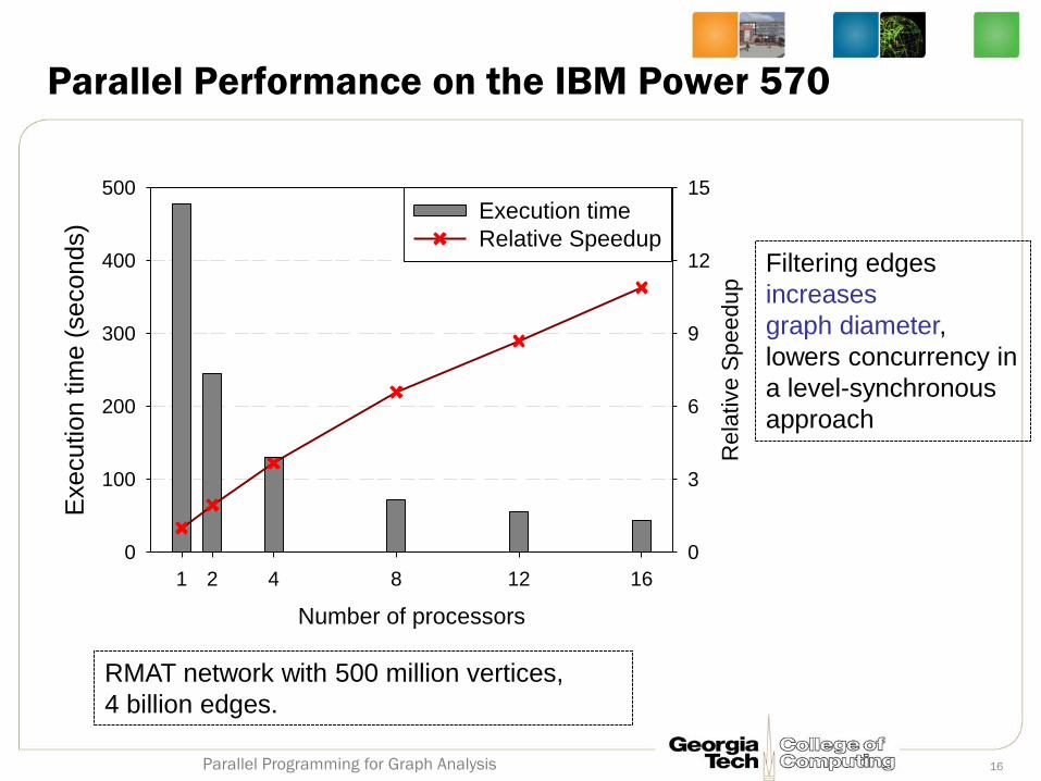
Parallel Performance on the IBM Power 570
RMAT network with 500 million vertices,
4 billion edges.
Filtering edges
increases
graph diameter,
lowers concurrency in
a level-synchronous
approach
Number of processors
1 2 4 8 12 16
Execution t
ime (
se
conds)
0
100
200
300
400
500
Rela
tive S
pee
dup
0
3
6
9
12
15
Execution time
Relative Speedup
16 Parallel Programming for Graph Analysis
STREAMING DATA ANALYSIS
17 Parallel Programming for Graph Analysis

Outline
• Background: Streaming Data Analysis
– Existing approaches do not meet current needs.
– Characteristics of data, problem, & related approaches
• Data structures for massive streaming graph analysis
– STINGER: Extensible, hybrid data structure supporting efficient, no-lock access
• Case study: Updating clustering coefficients, a localized graph metric
18 Parallel Programming for Graph Analysis
Background
• Streaming data analysis
– Known control & experimental paradigm
– New problem domains, unknown territory
• Characteristics
– Current data rates & unserved apps
– Irregular, partial, & massive data
– Archetypal questions
• Existing related, but different, topics
19 Parallel Programming for Graph Analysis
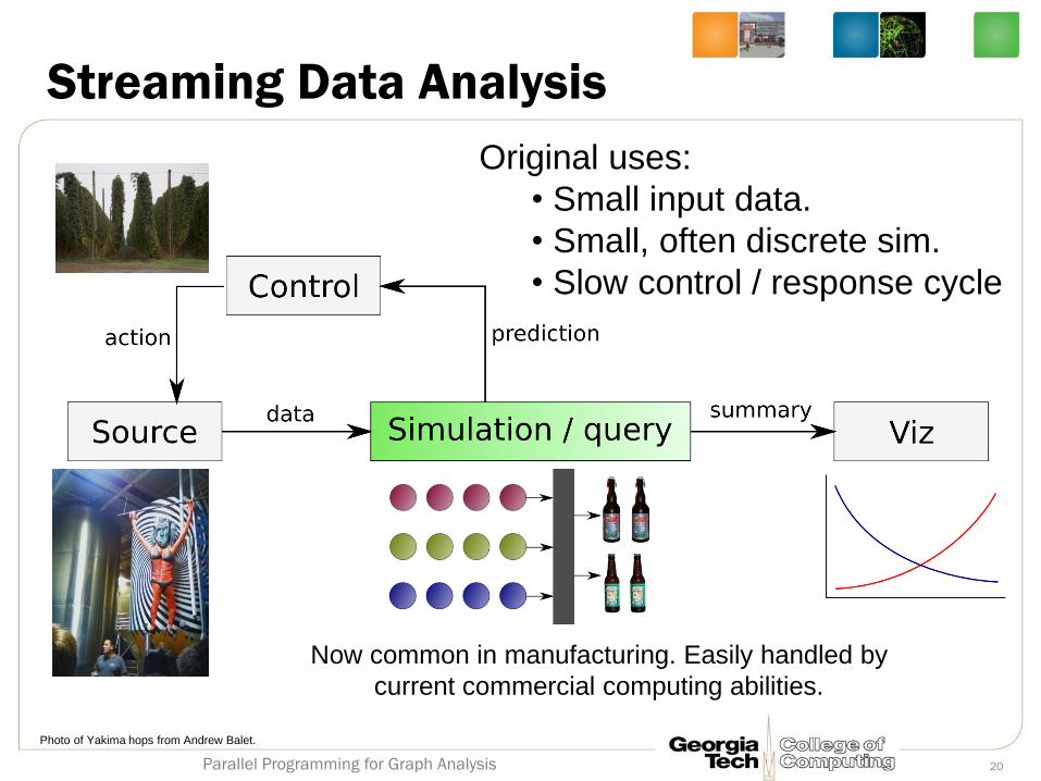
Streaming Data Analysis
Photo of Yakima hops from Andrew Balet.
Original uses:
• Small input data.
• Small, often discrete sim.
• Slow control / response cycle
Now common in manufacturing. Easily handled by
current commercial computing abilities.
20 Parallel Programming for Graph Analysis
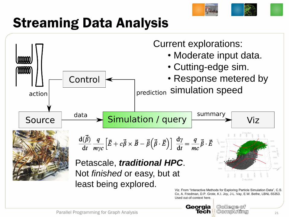
Streaming Data Analysis
Current explorations:
• Moderate input data.
• Cutting-edge sim.
• Response metered by
simulation speed
Petascale, traditional HPC.
Not finished or easy, but at
least being explored. Viz. From “Interactive Methods for Exploring Particle Simulation Data”, C.S.
Co, A. Friedman, D.P. Grote, K.I. Joy, J-L. Vay, E.W. Bethe, LBNL-55353.
Used out-of-context here.
21 Parallel Programming for Graph Analysis
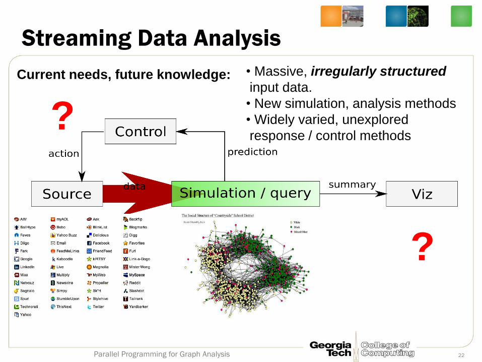
Streaming Data Analysis
• Massive, irregularly structured
input data.
• New simulation, analysis methods
• Widely varied, unexplored
response / control methods
?
?
Current needs, future knowledge:
22 Parallel Programming for Graph Analysis
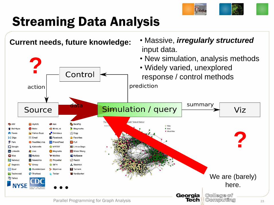
Streaming Data Analysis
• Massive, irregularly structured
input data.
• New simulation, analysis methods
• Widely varied, unexplored
response / control methods
?
?
Current needs, future knowledge:
We are (barely)
here. ... 23 Parallel Programming for Graph Analysis
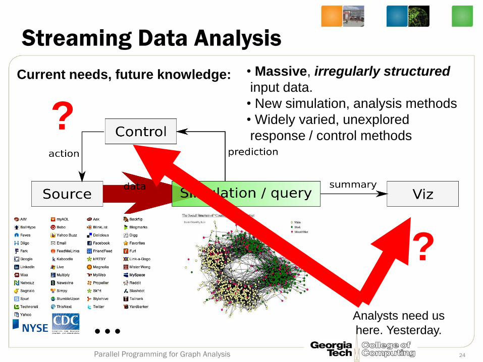
Streaming Data Analysis
• Massive, irregularly structured
input data.
• New simulation, analysis methods
• Widely varied, unexplored
response / control methods
?
?
Current needs, future knowledge:
Analysts need us
here. Yesterday. ... 24 Parallel Programming for Graph Analysis
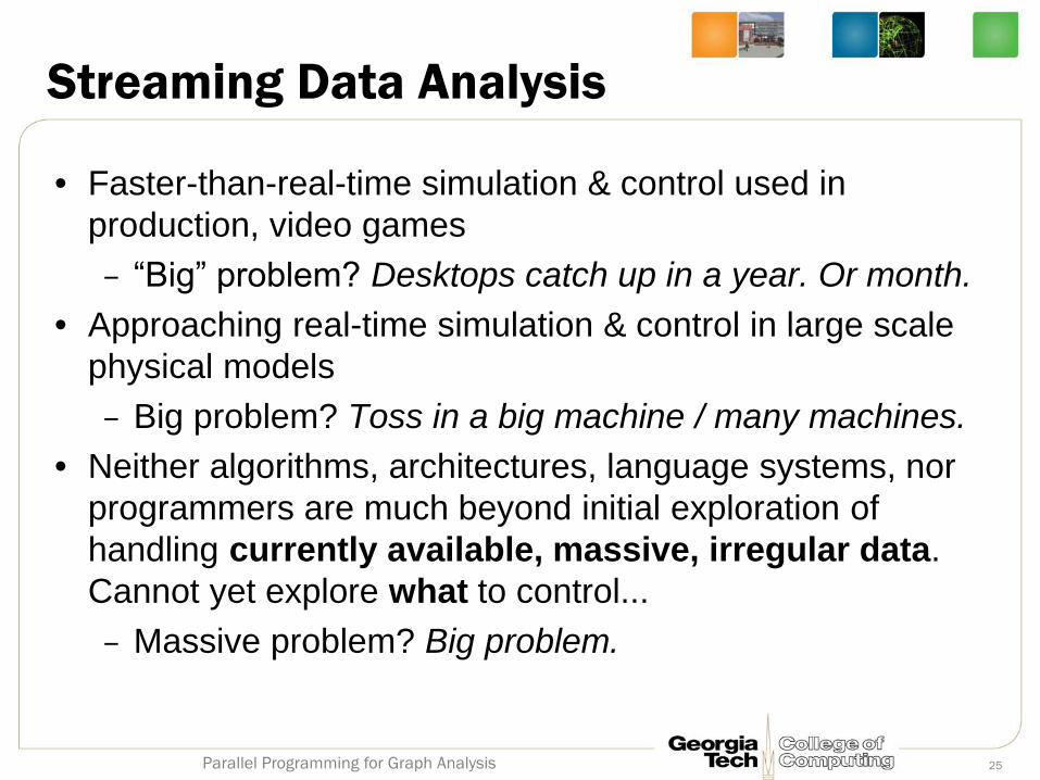
Streaming Data Analysis
• Faster-than-real-time simulation & control used in
production, video games
– “Big” problem? Desktops catch up in a year. Or month.
• Approaching real-time simulation & control in large scale
physical models
– Big problem? Toss in a big machine / many machines.
• Neither algorithms, architectures, language systems, nor
programmers are much beyond initial exploration of
handling currently available, massive, irregular data.
Cannot yet explore what to control...
– Massive problem? Big problem.
25 Parallel Programming for Graph Analysis
Current Example Data Rates
• Financial:
– NYSE processes 1.5TB daily, maintains 8PB
• Social:
– Facebook adds >100k users, 55M “status” updates, 80M
photos daily; more than 750M active users with an average of
130 “friend” connections each.
– Foursquare, a new service, reports 1.2M location check-ins per
week
• Scientific:
– MEDLINE adds from 1 to 140 publications a day
Shared features: All data is rich, irregularly connected to other data.
All is a mix of “good” and “bad” data... And much real data may
be missing or inconsistent.
26 Parallel Programming for Graph Analysis
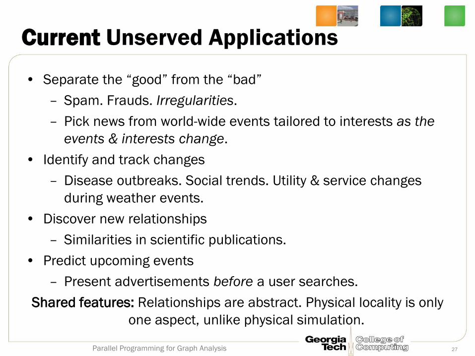
Current Unserved Applications
• Separate the “good” from the “bad”
– Spam. Frauds. Irregularities.
– Pick news from world-wide events tailored to interests as the
events & interests change.
• Identify and track changes
– Disease outbreaks. Social trends. Utility & service changes
during weather events.
• Discover new relationships
– Similarities in scientific publications.
• Predict upcoming events
– Present advertisements before a user searches.
Shared features: Relationships are abstract. Physical locality is only
one aspect, unlike physical simulation.
27 Parallel Programming for Graph Analysis
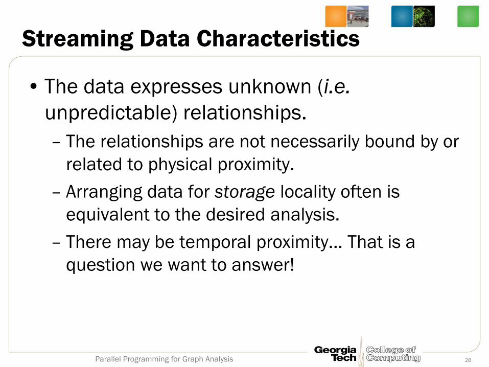
Streaming Data Characteristics
• The data expresses unknown (i.e.
unpredictable) relationships.
– The relationships are not necessarily bound by or
related to physical proximity.
– Arranging data for storage locality often is
equivalent to the desired analysis.
– There may be temporal proximity... That is a
question we want to answer!
28 Parallel Programming for Graph Analysis
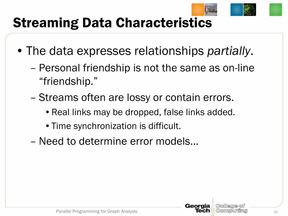
Streaming Data Characteristics
• The data expresses relationships partially.
– Personal friendship is not the same as on-line
“friendship.”
– Streams often are lossy or contain errors.
•Real links may be dropped, false links added.
•Time synchronization is difficult.
– Need to determine error models...
29 Parallel Programming for Graph Analysis
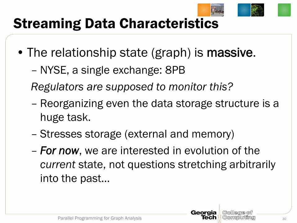
Streaming Data Characteristics
• The relationship state (graph) is massive.
– NYSE, a single exchange: 8PB
Regulators are supposed to monitor this?
– Reorganizing even the data storage structure is a
huge task.
– Stresses storage (external and memory)
– For now, we are interested in evolution of the
current state, not questions stretching arbitrarily
into the past...
30 Parallel Programming for Graph Analysis
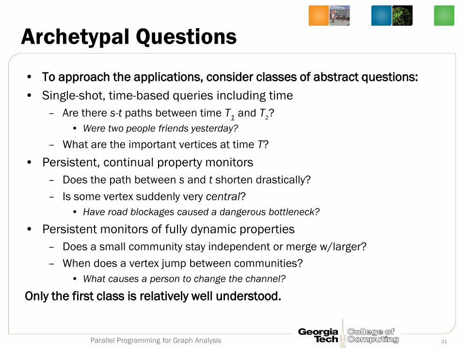
Archetypal Questions
• To approach the applications, consider classes of abstract questions:
• Single-shot, time-based queries including time
– Are there s-t paths between time T1 and T
2?
• Were two people friends yesterday?
– What are the important vertices at time T?
• Persistent, continual property monitors
– Does the path between s and t shorten drastically?
– Is some vertex suddenly very central?
• Have road blockages caused a dangerous bottleneck?
• Persistent monitors of fully dynamic properties
– Does a small community stay independent or merge w/larger?
– When does a vertex jump between communities?
• What causes a person to change the channel?
Only the first class is relatively well understood.
31 Parallel Programming for Graph Analysis
Related Research Topics
• Many related topics exist in the literature.
• None of these quite match the problem's
needs.
• But many of their results are just waiting to
be used and extended...
32 Parallel Programming for Graph Analysis
Related Research Topics
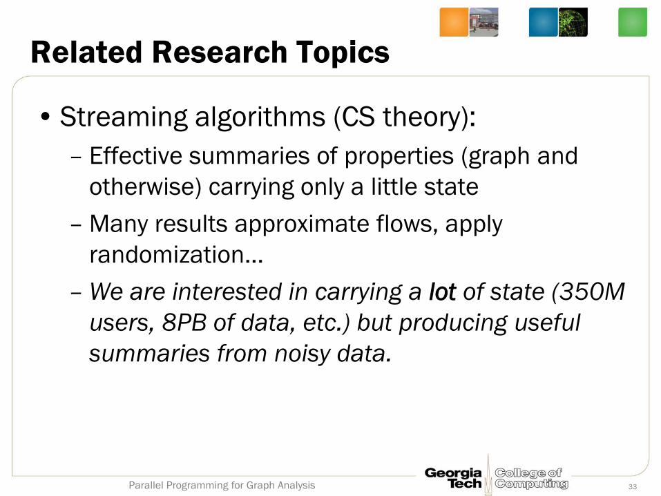
• Streaming algorithms (CS theory):
– Effective summaries of properties (graph and
otherwise) carrying only a little state
– Many results approximate flows, apply
randomization...
– We are interested in carrying a lot of state (350M
users, 8PB of data, etc.) but producing useful
summaries from noisy data.
33 Parallel Programming for Graph Analysis
Related Research Topics
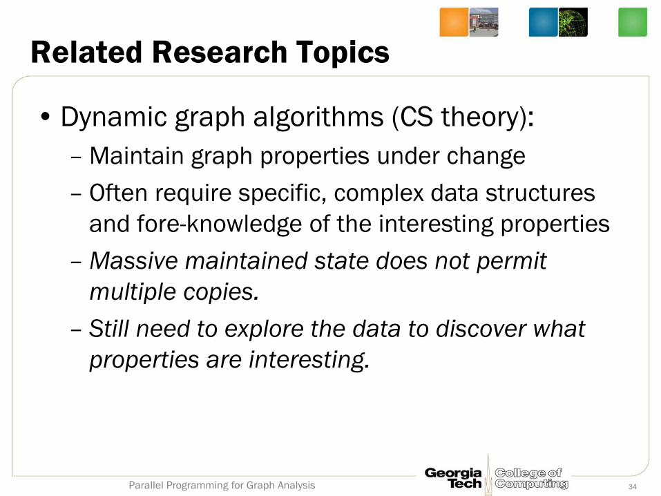
• Dynamic graph algorithms (CS theory):
– Maintain graph properties under change
– Often require specific, complex data structures
and fore-knowledge of the interesting properties
– Massive maintained state does not permit
multiple copies.
– Still need to explore the data to discover what
properties are interesting.
34 Parallel Programming for Graph Analysis
Related Research Topics
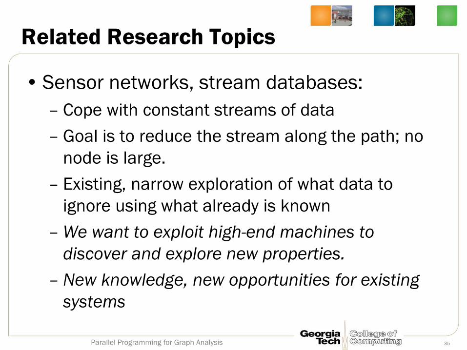
• Sensor networks, stream databases:
– Cope with constant streams of data
– Goal is to reduce the stream along the path; no
node is large.
– Existing, narrow exploration of what data to
ignore using what already is known
– We want to exploit high-end machines to
discover and explore new properties.
– New knowledge, new opportunities for existing
systems
35 Parallel Programming for Graph Analysis
Related Research Topics
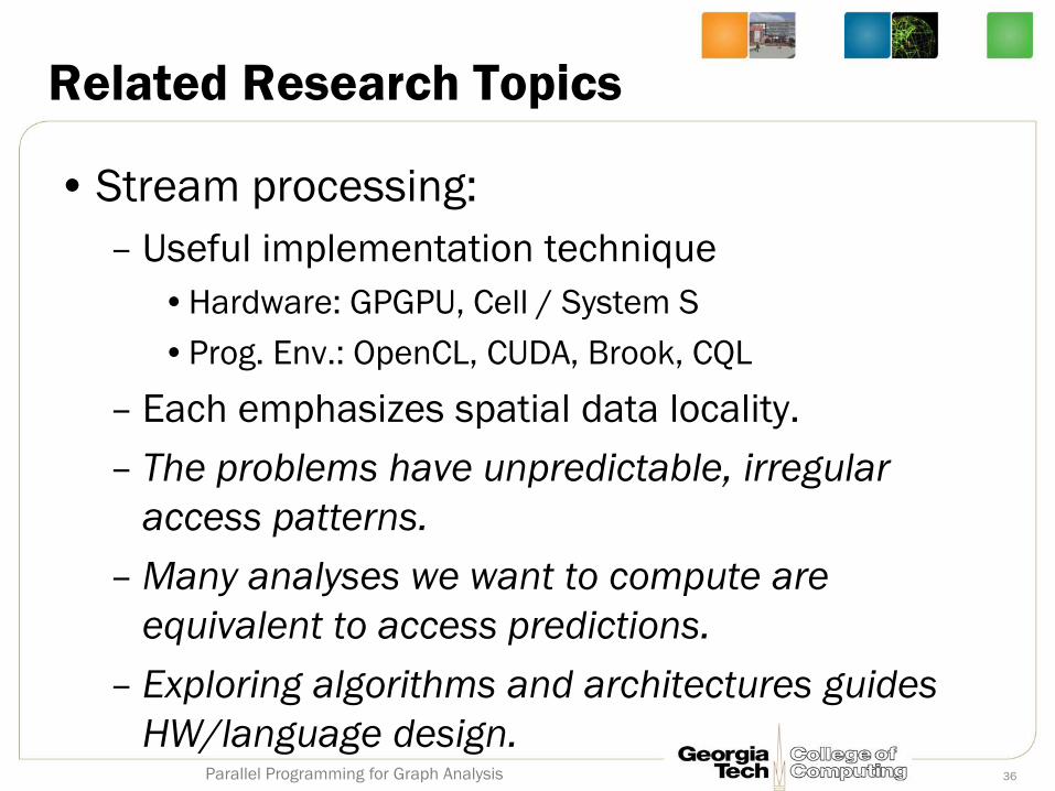
• Stream processing:
– Useful implementation technique
•Hardware: GPGPU, Cell / System S
•Prog. Env.: OpenCL, CUDA, Brook, CQL
– Each emphasizes spatial data locality.
– The problems have unpredictable, irregular
access patterns.
– Many analyses we want to compute are
equivalent to access predictions.
– Exploring algorithms and architectures guides
HW/language design. 36 Parallel Programming for Graph Analysis
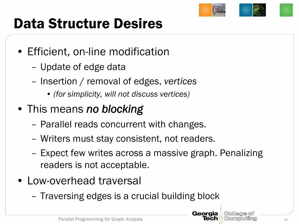
Data Structure Desires
• Efficient, on-line modification
– Update of edge data
– Insertion / removal of edges, vertices
• (for simplicity, will not discuss vertices)
• This means no blocking
– Parallel reads concurrent with changes.
– Writers must stay consistent, not readers.
– Expect few writes across a massive graph. Penalizing
readers is not acceptable.
• Low-overhead traversal
– Traversing edges is a crucial building block
37 Parallel Programming for Graph Analysis
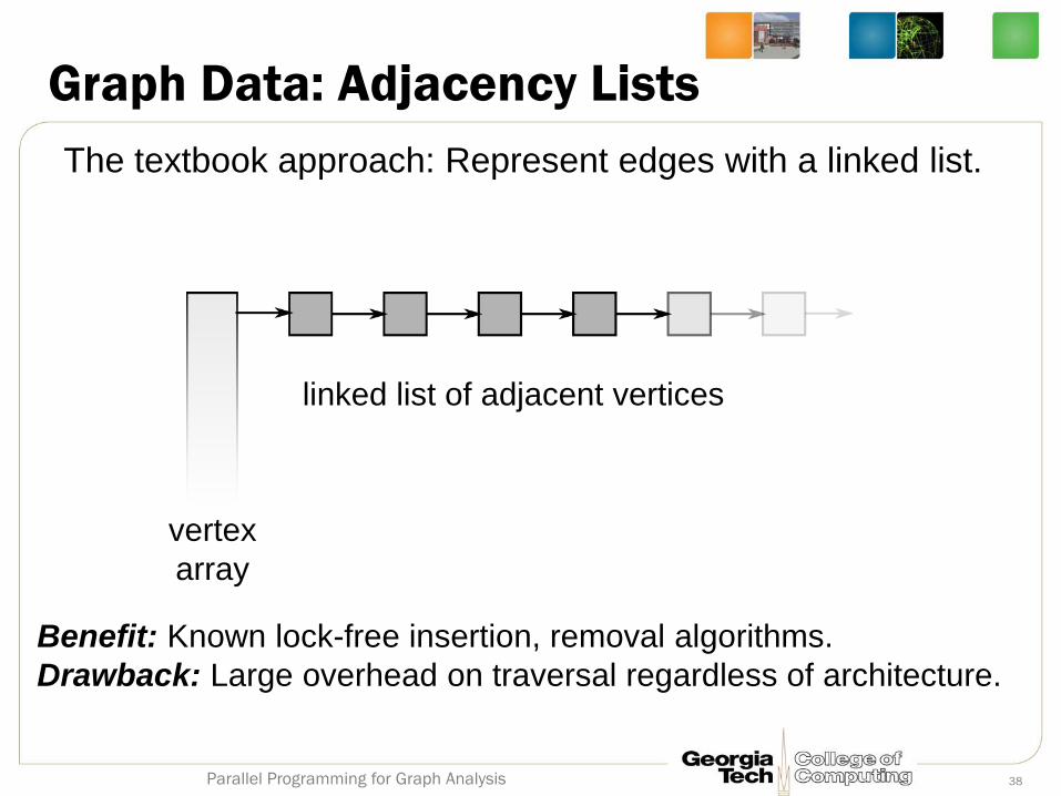
Graph Data: Adjacency Lists
The textbook approach: Represent edges with a linked list.
vertex
array
linked list of adjacent vertices
Benefit: Known lock-free insertion, removal algorithms.
Drawback: Large overhead on traversal regardless of architecture.
38 Parallel Programming for Graph Analysis
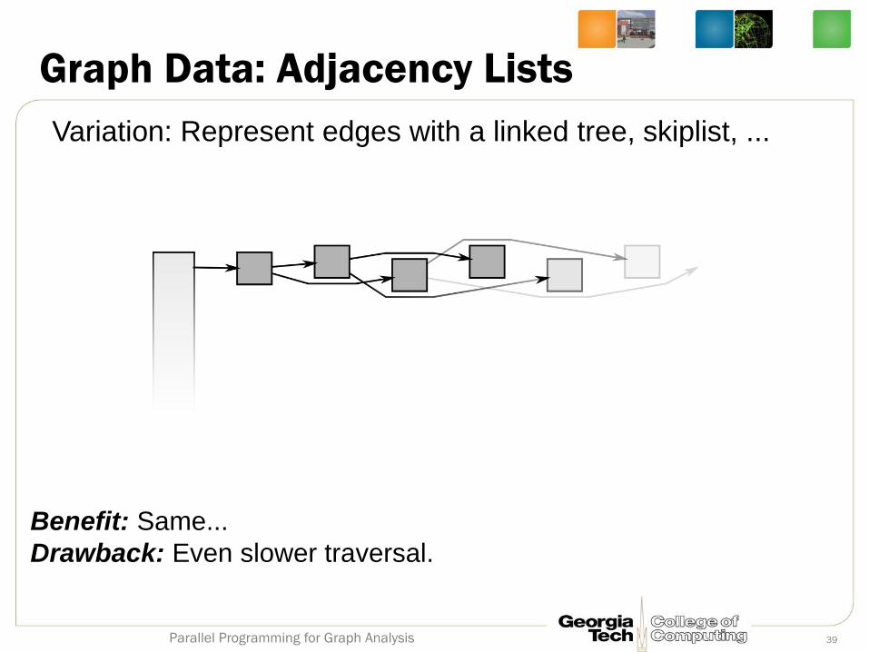
Graph Data: Adjacency Lists
Variation: Represent edges with a linked tree, skiplist, ...
Benefit: Same...
Drawback: Even slower traversal.
39 Parallel Programming for Graph Analysis
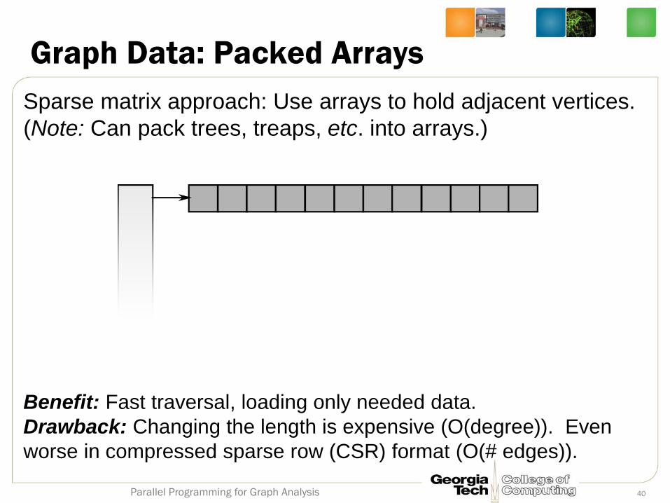
Graph Data: Packed Arrays
Sparse matrix approach: Use arrays to hold adjacent vertices.
(Note: Can pack trees, treaps, etc. into arrays.)
Benefit: Fast traversal, loading only needed data.
Drawback: Changing the length is expensive (O(degree)). Even
worse in compressed sparse row (CSR) format (O(# edges)).
40 Parallel Programming for Graph Analysis
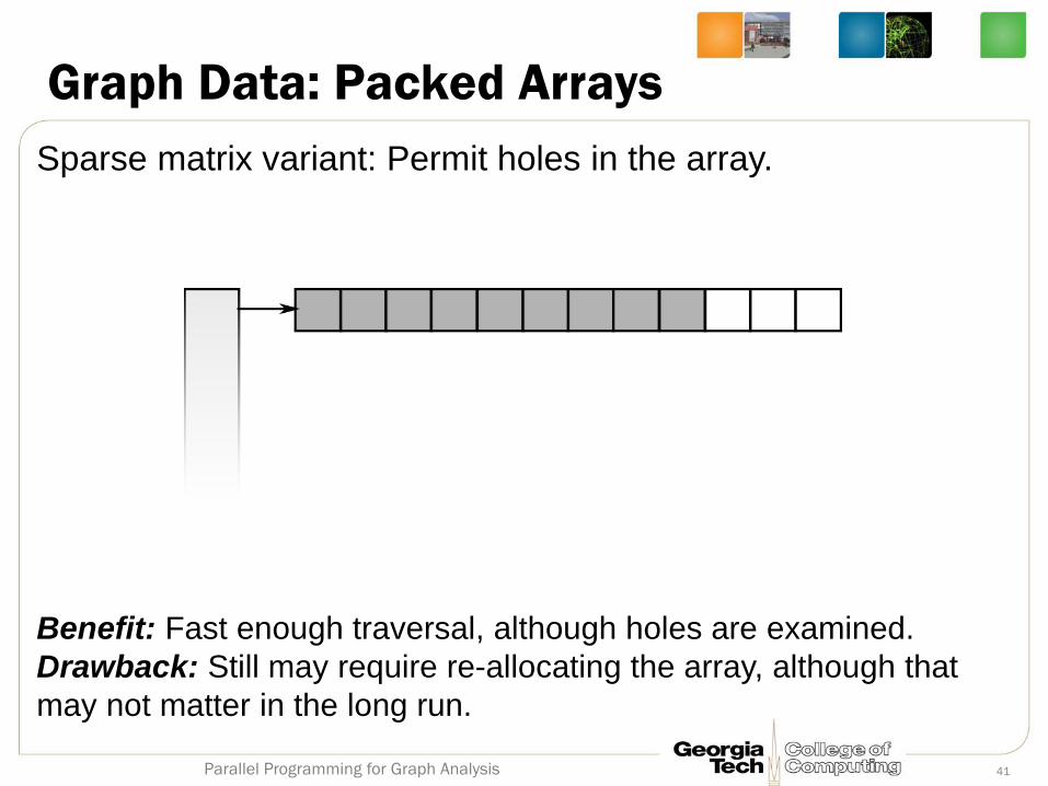
Graph Data: Packed Arrays
Sparse matrix variant: Permit holes in the array.
Benefit: Fast enough traversal, although holes are examined.
Drawback: Still may require re-allocating the array, although that
may not matter in the long run.
41 Parallel Programming for Graph Analysis
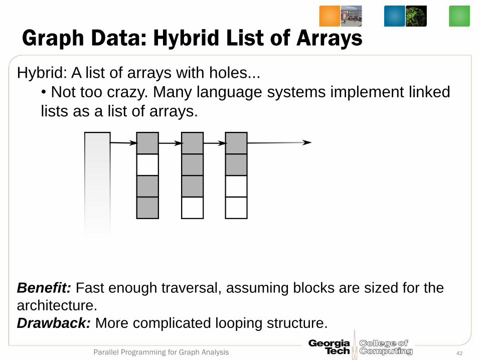
Graph Data: Hybrid List of Arrays
Hybrid: A list of arrays with holes...
• Not too crazy. Many language systems implement linked
lists as a list of arrays.
Benefit: Fast enough traversal, assuming blocks are sized for the
architecture.
Drawback: More complicated looping structure.
42 Parallel Programming for Graph Analysis
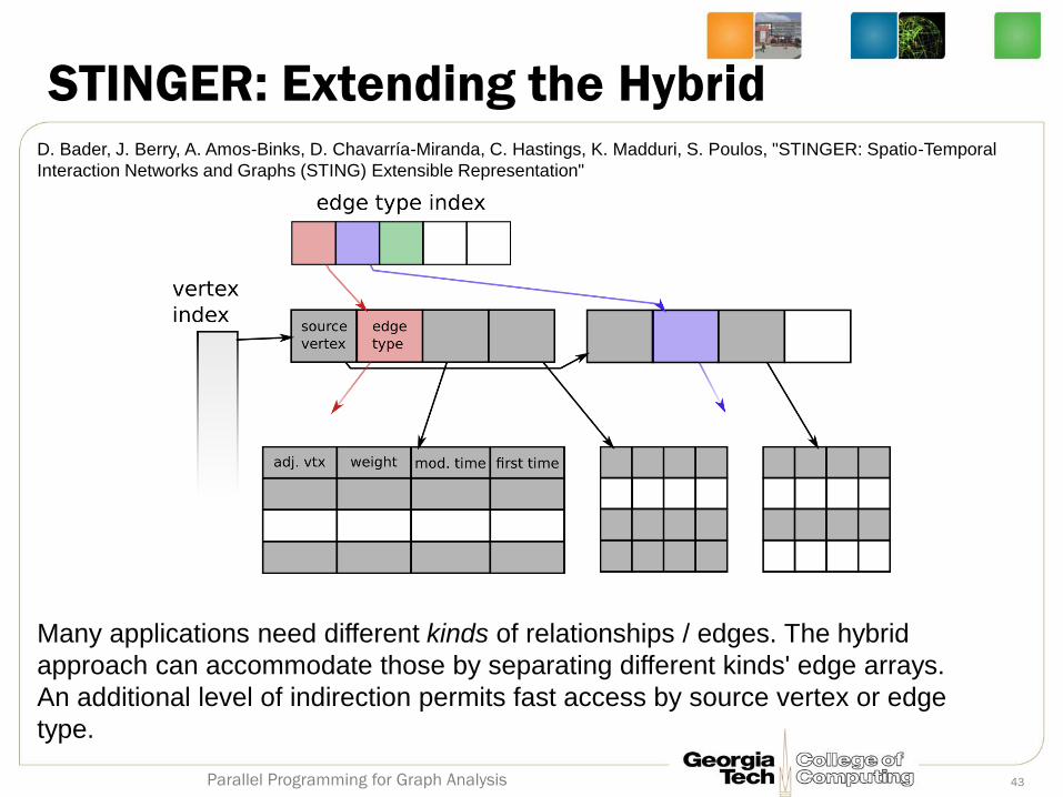
STINGER: Extending the Hybrid
Many applications need different kinds of relationships / edges. The hybrid
approach can accommodate those by separating different kinds' edge arrays.
An additional level of indirection permits fast access by source vertex or edge
type.
D. Bader, J. Berry, A. Amos-Binks, D. Chavarría-Miranda, C. Hastings, K. Madduri, S. Poulos, "STINGER: Spatio-Temporal
Interaction Networks and Graphs (STING) Extensible Representation"
43 Parallel Programming for Graph Analysis
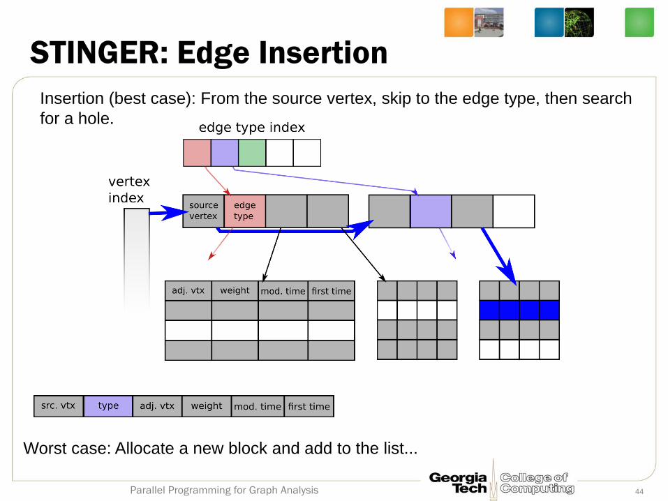
STINGER: Edge Insertion
Insertion (best case): From the source vertex, skip to the edge type, then search
for a hole.
Worst case: Allocate a new block and add to the list...
44 Parallel Programming for Graph Analysis
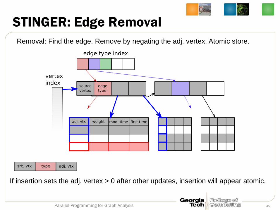
STINGER: Edge Removal
Removal: Find the edge. Remove by negating the adj. vertex. Atomic store.
If insertion sets the adj. vertex > 0 after other updates, insertion will appear atomic.
45 Parallel Programming for Graph Analysis
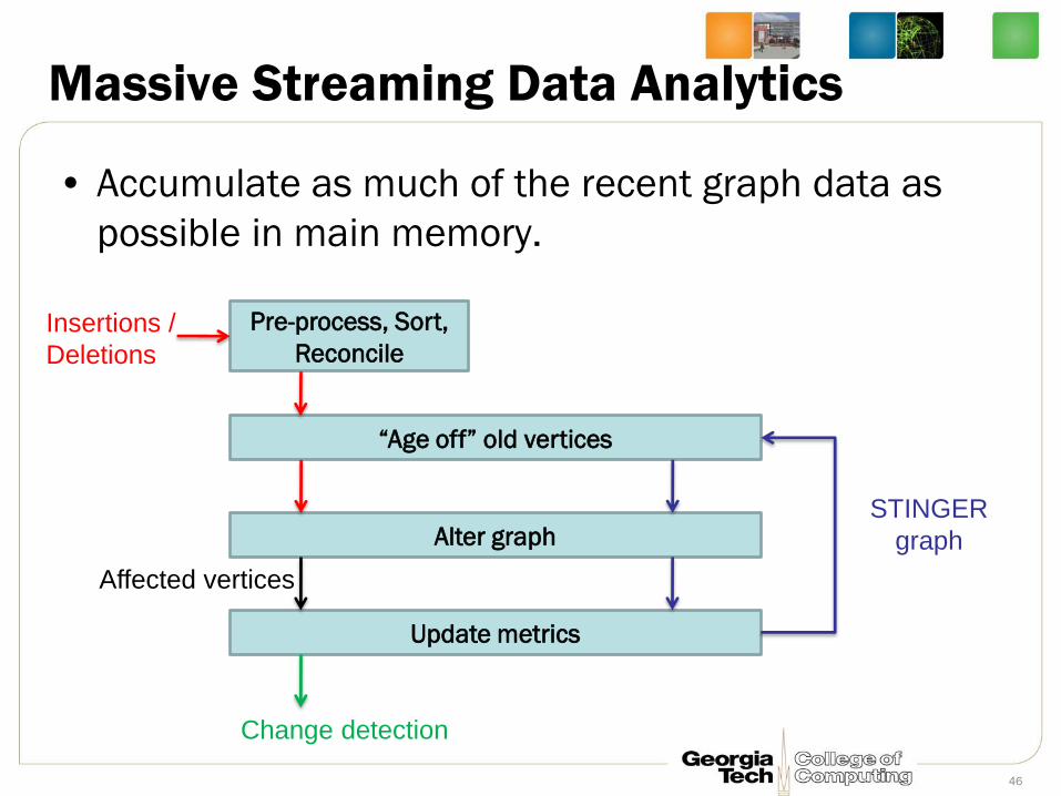
Massive Streaming Data Analytics
• Accumulate as much of the recent graph data as
possible in main memory.
46
Pre-process, Sort,
Reconcile
“Age off” old vertices
Alter graph
Update metrics
STINGER
graph
Insertions /
Deletions
Affected vertices
Change detection
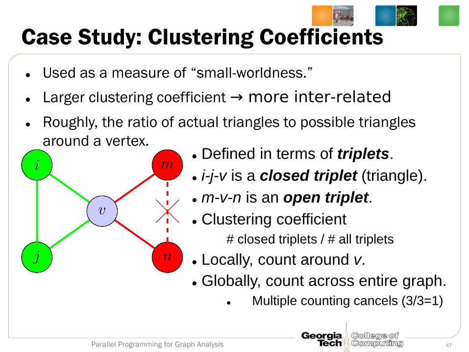
Case Study: Clustering Coefficients
Used as a measure of “small-worldness.”
Larger clustering coefficient → more inter-related
Roughly, the ratio of actual triangles to possible triangles
around a vertex. Defined in terms of triplets.
i-j-v is a closed triplet (triangle).
m-v-n is an open triplet.
Clustering coefficient
# closed triplets / # all triplets
Locally, count around v.
Globally, count across entire graph.
Multiple counting cancels (3/3=1)
47 Parallel Programming for Graph Analysis
Batching Graph Changes
Individual graph changes for local properties will not expose
much parallelism. Need to consider many actions at once
for performance.
Conveniently, batches of actions also amortize transfer
overhead from the data source.
Common paradigm in network servers (c.f. SEDA: Staged Event-
Driven Arch.)
Even more conveniently, clustering coefficients lend
themselves to batches.
Final result independent of action ordering between edges.
Can reconcile all actions on a single edge within the batch.
48 Parallel Programming for Graph Analysis
Streaming updates to clustering coefficients
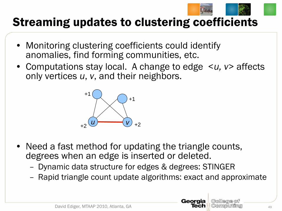
• Monitoring clustering coefficients could identify anomalies, find forming communities, etc.
• Computations stay local. A change to edge <u, v> affects only vertices u, v, and their neighbors.
• Need a fast method for updating the triangle counts, degrees when an edge is inserted or deleted. – Dynamic data structure for edges & degrees: STINGER
– Rapid triangle count update algorithms: exact and approximate
+2 u v +2
+1 +1
David Ediger, MTAAP 2010, Atlanta, GA 49
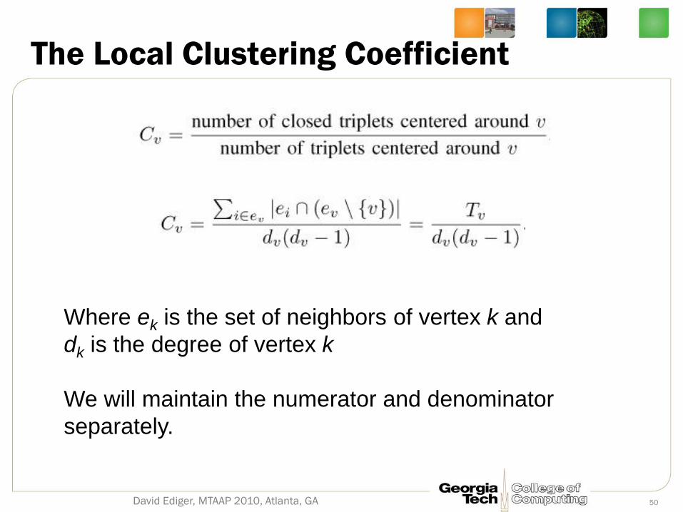
The Local Clustering Coefficient
David Ediger, MTAAP 2010, Atlanta, GA
Where ek is the set of neighbors of vertex k and
dk is the degree of vertex k
We will maintain the numerator and denominator
separately.
50
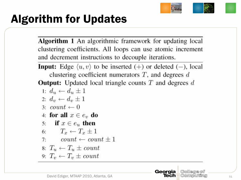
Algorithm for Updates
David Ediger, MTAAP 2010, Atlanta, GA 51
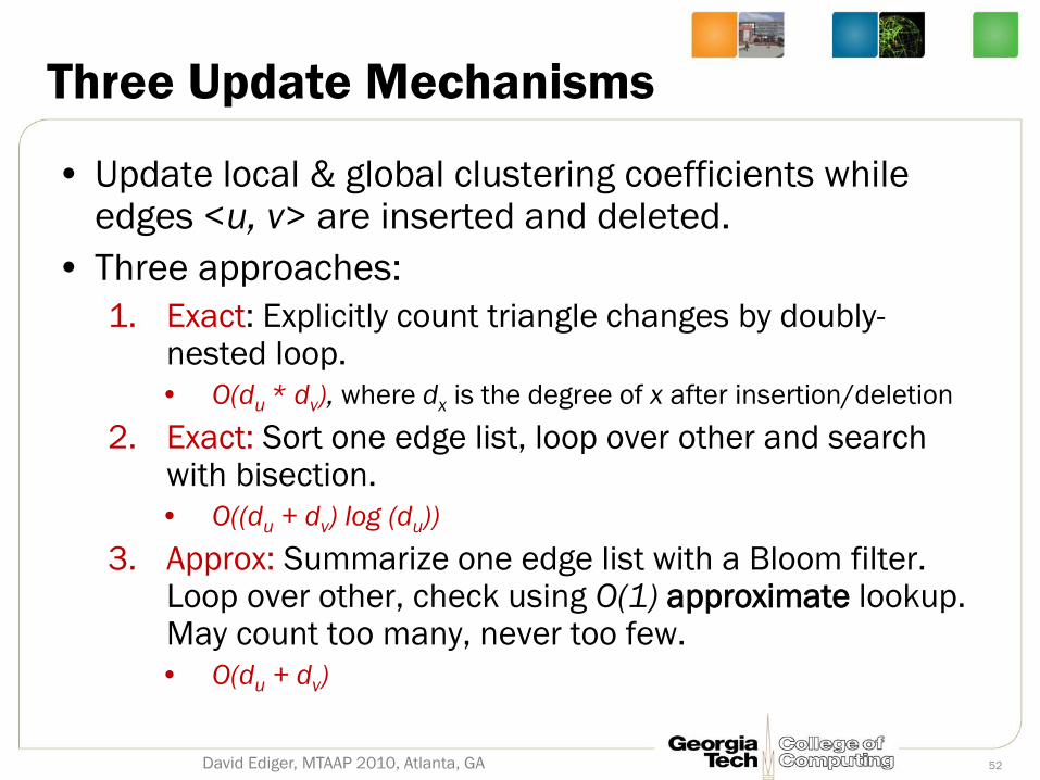
Three Update Mechanisms
• Update local & global clustering coefficients while edges <u, v> are inserted and deleted.
• Three approaches:
1. Exact: Explicitly count triangle changes by doubly-nested loop.
• O(du * dv), where dx is the degree of x after insertion/deletion
2. Exact: Sort one edge list, loop over other and search with bisection.
• O((du + dv) log (du))
3. Approx: Summarize one edge list with a Bloom filter. Loop over other, check using O(1) approximate lookup. May count too many, never too few.
• O(du + dv)
David Ediger, MTAAP 2010, Atlanta, GA 52
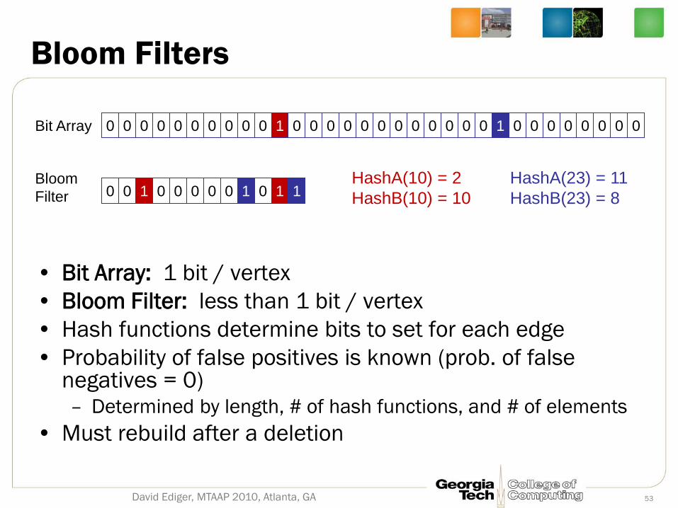
Bloom Filters
• Bit Array: 1 bit / vertex
• Bloom Filter: less than 1 bit / vertex
• Hash functions determine bits to set for each edge
• Probability of false positives is known (prob. of false negatives = 0) – Determined by length, # of hash functions, and # of elements
• Must rebuild after a deletion
David Ediger, MTAAP 2010, Atlanta, GA 53
0 0 0 0 0 0 0 0 0 0 1 0 0 0 0 0 0 0 0 0 0 0 0 1 0 0 0 0 0 0 0 0
0 0 1 0 0 0 0 0 1 0 1 1 HashA(10) = 2
HashB(10) = 10
HashA(23) = 11
HashB(23) = 8
Bit Array
Bloom
Filter
Updating Triplet Counts
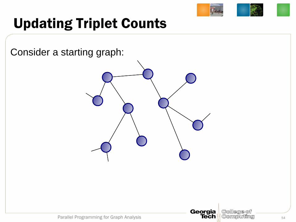
Consider a starting graph:
54 Parallel Programming for Graph Analysis
Updating Triplet Counts
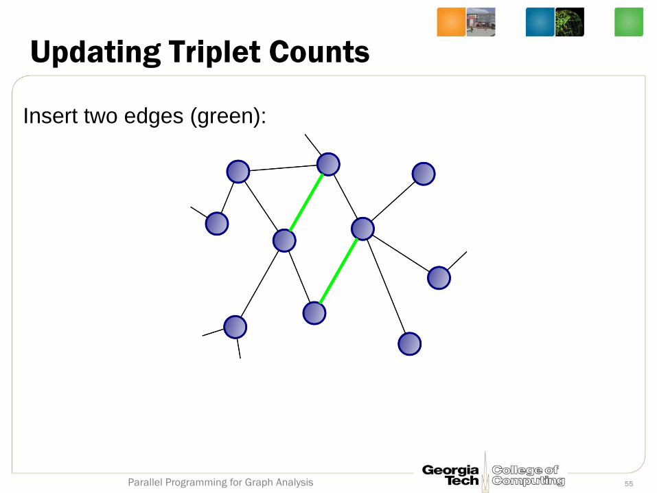
Insert two edges (green):
55 Parallel Programming for Graph Analysis
Updating Triplet Counts
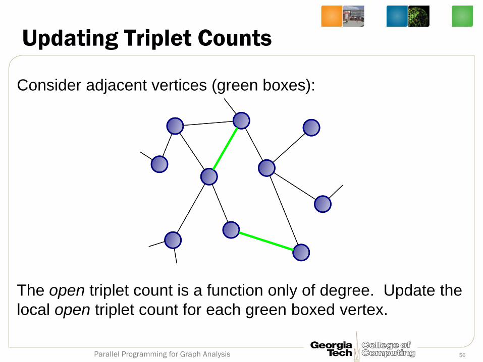
Consider adjacent vertices (green boxes):
The open triplet count is a function only of degree. Update the
local open triplet count for each green boxed vertex.
56 Parallel Programming for Graph Analysis
Updating Triplet Counts
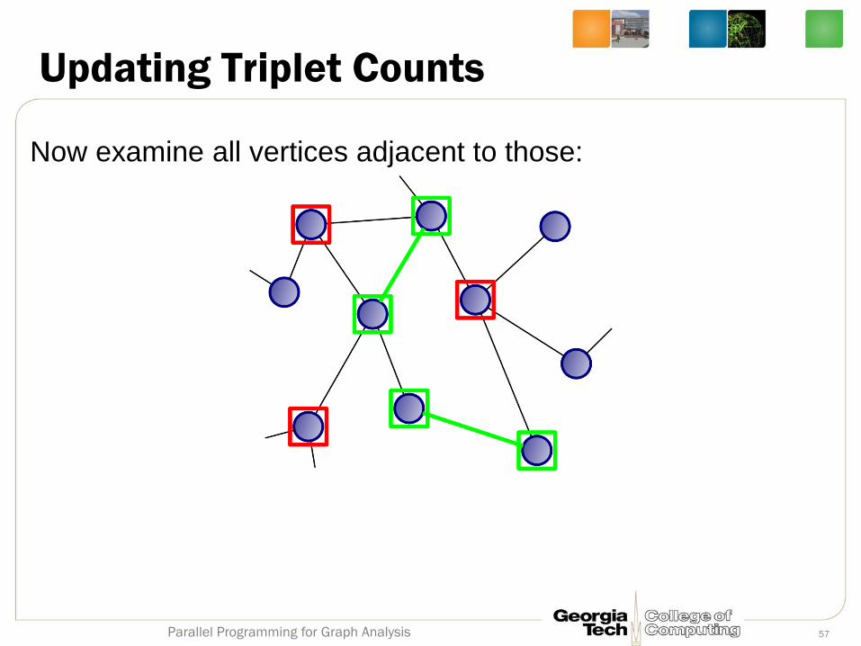
Now examine all vertices adjacent to those:
57 Parallel Programming for Graph Analysis
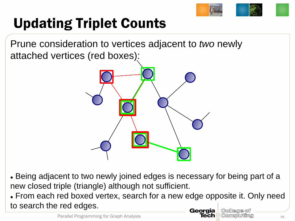
Updating Triplet Counts
Prune consideration to vertices adjacent to two newly
attached vertices (red boxes):
Being adjacent to two newly joined edges is necessary for being part of a
new closed triple (triangle) although not sufficient.
From each red boxed vertex, search for a new edge opposite it. Only need
to search the red edges.
58 Parallel Programming for Graph Analysis
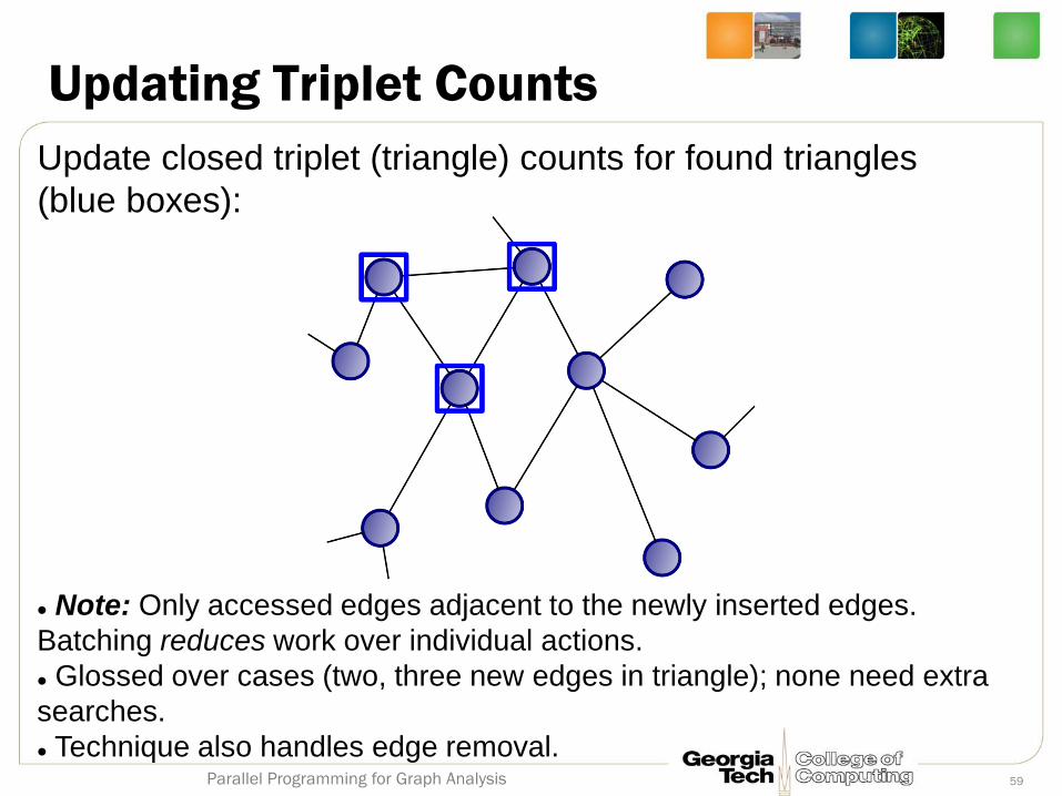
Updating Triplet Counts
Update closed triplet (triangle) counts for found triangles
(blue boxes):
Note: Only accessed edges adjacent to the newly inserted edges.
Batching reduces work over individual actions.
Glossed over cases (two, three new edges in triangle); none need extra
searches.
Technique also handles edge removal. 59 Parallel Programming for Graph Analysis
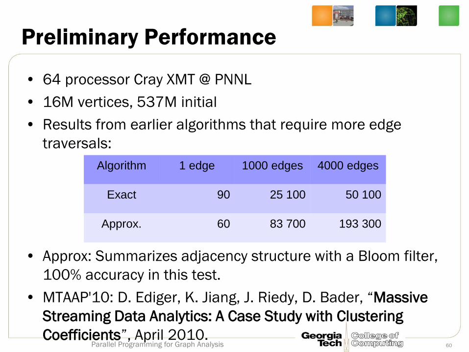
Preliminary Performance
• 64 processor Cray XMT @ PNNL
• 16M vertices, 537M initial
• Results from earlier algorithms that require more edge
traversals:
• Approx: Summarizes adjacency structure with a Bloom filter,
100% accuracy in this test.
• MTAAP'10: D. Ediger, K. Jiang, J. Riedy, D. Bader, “Massive
Streaming Data Analytics: A Case Study with Clustering
Coefficients”, April 2010.
Algorithm 1 edge 1000 edges 4000 edges
Exact 90 25 100 50 100
Approx. 60 83 700 193 300
60 Parallel Programming for Graph Analysis
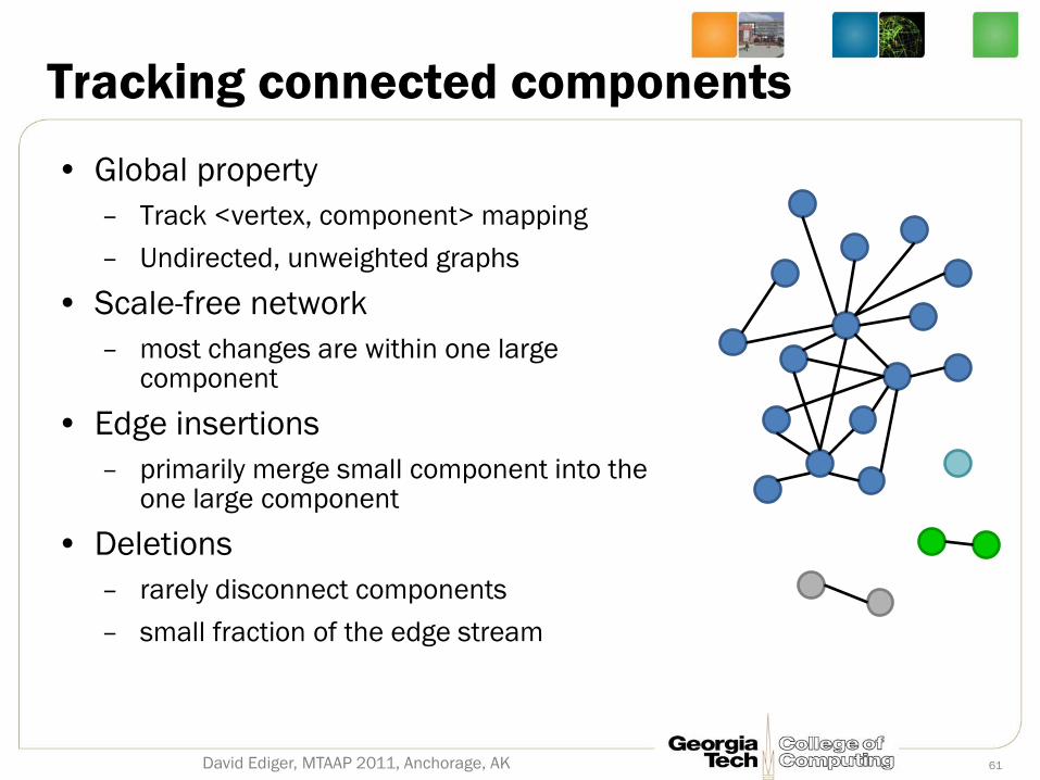
Tracking connected components
• Global property
– Track <vertex, component> mapping
– Undirected, unweighted graphs
• Scale-free network
– most changes are within one large component
• Edge insertions
– primarily merge small component into the one large component
• Deletions
– rarely disconnect components
– small fraction of the edge stream
61 David Ediger, MTAAP 2011, Anchorage, AK
Insertions-only connected components algorithm
Edge insertion (in batches):
• Relabel batch of insertions with component numbers.
• Collapse the graph, removing self-edges. Any edges that remain cross components.
• Compute components of component ↔ component graph. Relabel smaller into larger.
• Problem size reduces from number of changes to number of components.
• Can proceed concurrently with STINGER modification.
62 David Ediger, MTAAP 2011, Anchorage, AK
The Problem with Deletions
• An edge insertion contains local information about
connectivity
– Insert(u, v) = u and v are connected
• An edge deletion cannot always determine locally if
a component has disconnected
– Delete(u, v) = non-existence of edge between u & v
• Re-establishing connectivity after a deletion could
be a global operation
David Ediger, MTAAP 2011, Anchorage, AK 63
Related Work
• Shiloach & Even (1981): Two breadth-first searches
– 1st to restablish connectivity, 2nd to find separation
• Eppstein et al. (1997): Partition according to degree
• Henzinger, King, Warnow (1999): Sequence & coloring
• Henzinger & King (1999): Partition dense to sparse
– Start BFS in the densest subgraph and move up
• Roditty & Zwick (2004): Sequence of graphs
• Conclusion: In the worst case, graph traversal per deletion is
expensive. Use heuristics to avoid it, if possible.
David Ediger, MTAAP 2011, Anchorage, AK 64
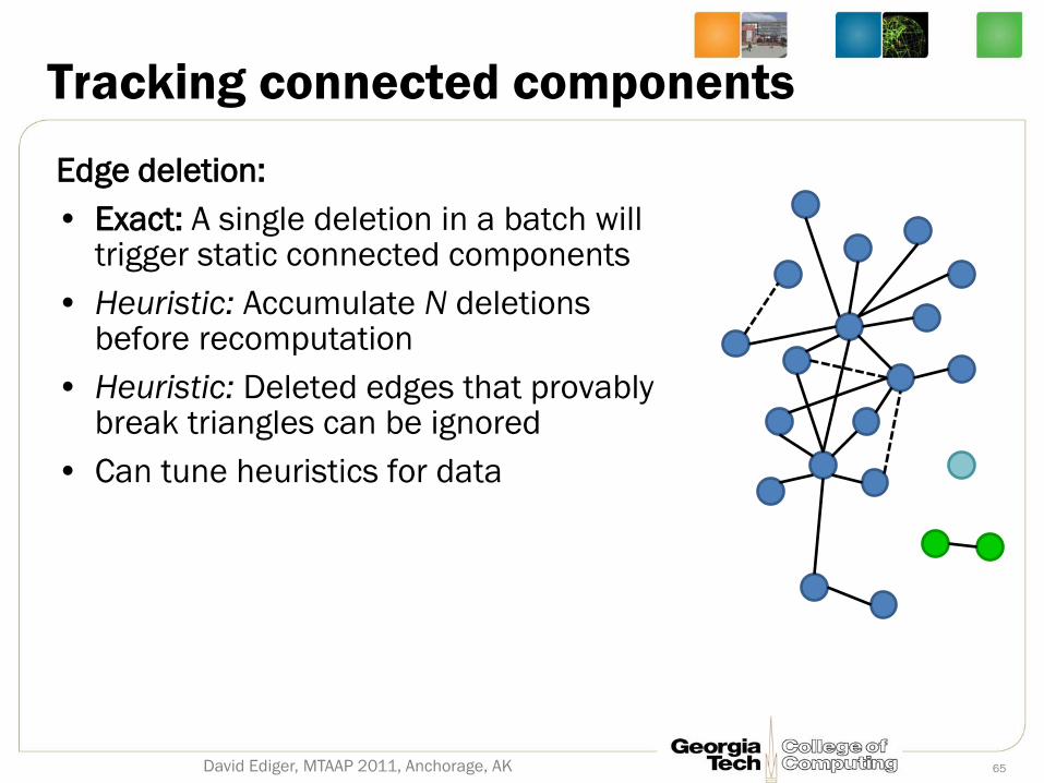
Tracking connected components
Edge deletion:
• Exact: A single deletion in a batch will trigger static connected components
• Heuristic: Accumulate N deletions before recomputation
• Heuristic: Deleted edges that provably break triangles can be ignored
• Can tune heuristics for data
65 David Ediger, MTAAP 2011, Anchorage, AK
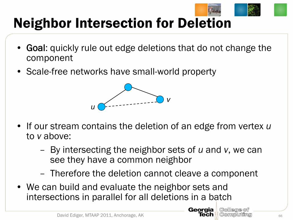
Neighbor Intersection for Deletion
• Goal: quickly rule out edge deletions that do not change the component
• Scale-free networks have small-world property
• If our stream contains the deletion of an edge from vertex u to v above:
– By intersecting the neighbor sets of u and v, we can see they have a common neighbor
– Therefore the deletion cannot cleave a component
• We can build and evaluate the neighbor sets and intersections in parallel for all deletions in a batch
David Ediger, MTAAP 2011, Anchorage, AK 66
u v
Algorithm for Bit Array Intersection
• For each unique source vertex in the batch (in parallel)
– Compute a bit array representing the neighbor list
• Relatively few to construct because of power law dist.
• Perform the deletions in STINGER
• For each destination vertex in the batch (in parallel)
– For each neighbor, query the bit array of the source
– Any common neighbor means the component did not change
• This technique reduces the number of edge deletions that could cause structural change by an order of magnitude in preliminary investigations.
– Example: ~7000 → ~700 for batches of 100k edges
– Actual # of relevant deletions: ~10
David Ediger, MTAAP 2011, Anchorage, AK 67
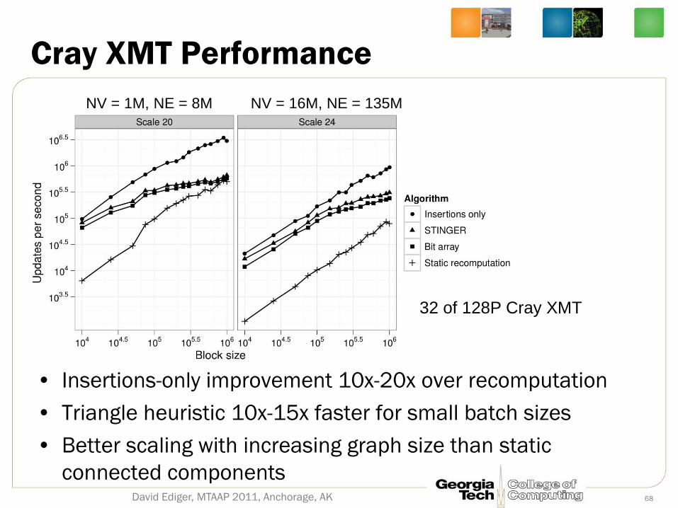
Cray XMT Performance
David Ediger, MTAAP 2011, Anchorage, AK 68
32 of 128P Cray XMT
NV = 1M, NE = 8M NV = 16M, NE = 135M
• Insertions-only improvement 10x-20x over recomputation
• Triangle heuristic 10x-15x faster for small batch sizes
• Better scaling with increasing graph size than static
connected components
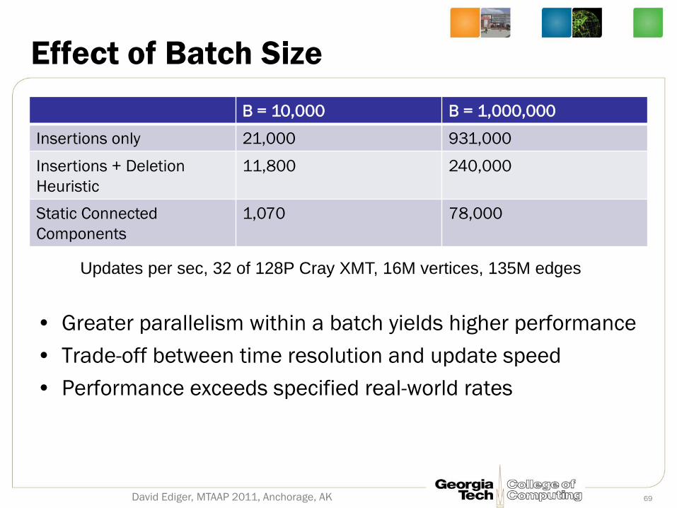
Effect of Batch Size
B = 10,000 B = 1,000,000
Insertions only 21,000 931,000
Insertions + Deletion
Heuristic
11,800 240,000
Static Connected
Components
1,070 78,000
David Ediger, MTAAP 2011, Anchorage, AK 69
Updates per sec, 32 of 128P Cray XMT, 16M vertices, 135M edges
• Greater parallelism within a batch yields higher performance
• Trade-off between time resolution and update speed
• Performance exceeds specified real-world rates
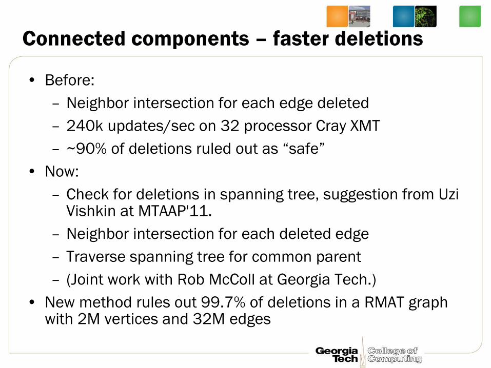
Connected components – faster deletions
• Before:
– Neighbor intersection for each edge deleted
– 240k updates/sec on 32 processor Cray XMT
– ~90% of deletions ruled out as “safe”
• Now:
– Check for deletions in spanning tree, suggestion from Uzi Vishkin at MTAAP'11.
– Neighbor intersection for each deleted edge
– Traverse spanning tree for common parent
– (Joint work with Rob McColl at Georgia Tech.)
• New method rules out 99.7% of deletions in a RMAT graph with 2M vertices and 32M edges
8
2 0
8 8 8 3 3 6 6 8 8 3
8 2 8 3 3 6 6 8 4 8
1
7
9 4
3
5
6
Vertex-component map
Spanning tree
V = 0 1 2 3 4 5 6 7 8 9
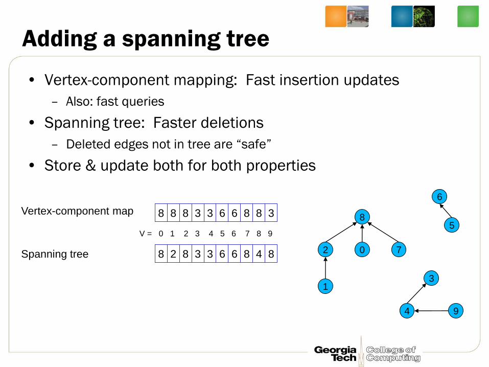
Adding a spanning tree
• Vertex-component mapping: Fast insertion updates
– Also: fast queries
• Spanning tree: Faster deletions
– Deleted edges not in tree are “safe”
• Store & update both for both properties
Spanning Tree Edge
Non-Tree Edge
Root vertex in black
X
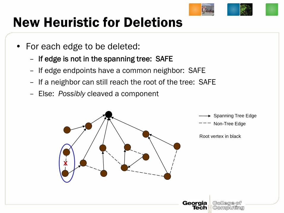
New Heuristic for Deletions
• For each edge to be deleted:
– If edge is not in the spanning tree: SAFE
– If edge endpoints have a common neighbor: SAFE
– If a neighbor can still reach the root of the tree: SAFE
– Else: Possibly cleaved a component
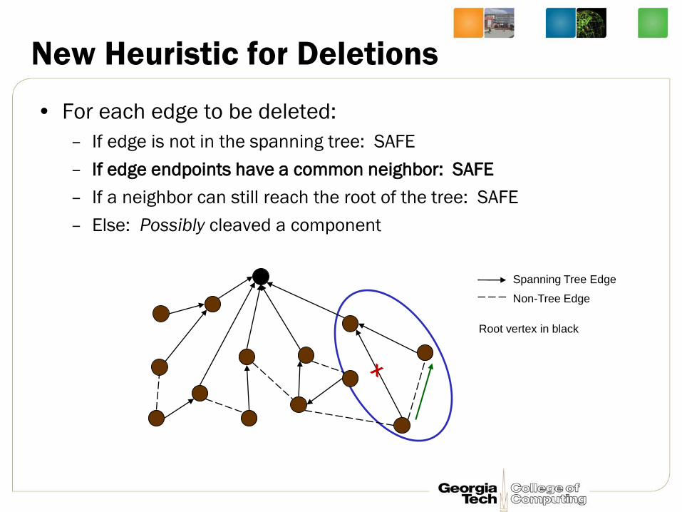
Spanning Tree Edge
Non-Tree Edge
Root vertex in black
New Heuristic for Deletions
• For each edge to be deleted:
– If edge is not in the spanning tree: SAFE
– If edge endpoints have a common neighbor: SAFE
– If a neighbor can still reach the root of the tree: SAFE
– Else: Possibly cleaved a component
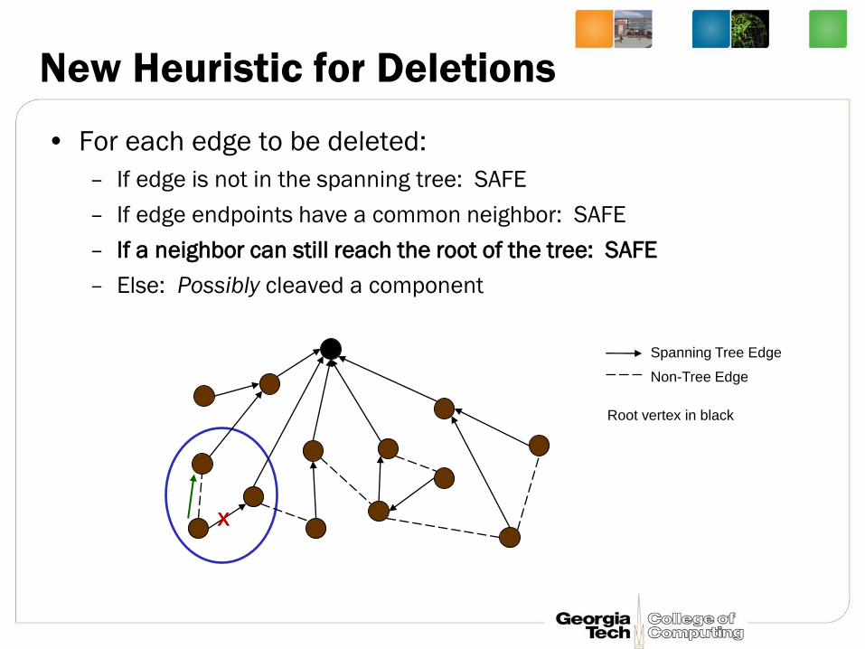
Spanning Tree Edge
Non-Tree Edge
Root vertex in black
X
New Heuristic for Deletions
• For each edge to be deleted:
– If edge is not in the spanning tree: SAFE
– If edge endpoints have a common neighbor: SAFE
– If a neighbor can still reach the root of the tree: SAFE
– Else: Possibly cleaved a component
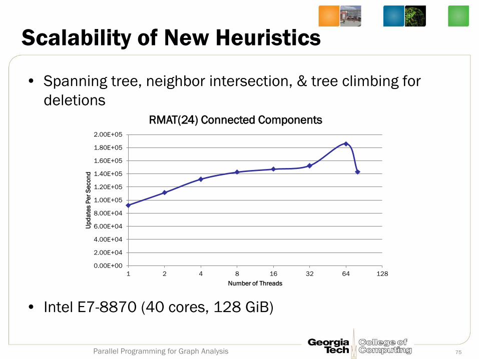
Scalability of New Heuristics
• Spanning tree, neighbor intersection, & tree climbing for
deletions
• Intel E7-8870 (40 cores, 128 GiB)
Parallel Programming for Graph Analysis 75
0.00E+00
2.00E+04
4.00E+04
6.00E+04
8.00E+04
1.00E+05
1.20E+05
1.40E+05
1.60E+05
1.80E+05
2.00E+05
1 2 4 8 16 32 64 128
Up
da
tes P
er
Se
co
nd
Number of Threads
RMAT(24) Connected Components
Q&A
Parallel Programming for Graph Analysis 76