5/3/14

1

STAT 342!

Peter Guttorp!

Outline!

χ2, F and t-distributions (Ch. 7)!Least squares and regression (Ch.11)!Analysis of variance (Ch. 12)!Goodness of fit (Ch. 10)!Ranks and order statistics (Ch. 14)!Bayesian statistics!Dependent data!!

P-value project!

The class will be divided into groups!Each group reads and discusses a paper on P-values!Write a commentary!Present your discussion to the class!

χ2-distribution!

Z~N(0,1)!P(Z2 ≤ z)!

fZ2 (z) =12 z

(φ( z ) + φ(− z))

5/3/14

2

Sum of squares of standard normals!

!!!k is called “degrees of freedom”!!Applet!

fZi2

1

k

∑(z) = x

k2−1e −x/2

2k2Γ(k2)

,x > 0

Friedrich Robert! Helmert 1843-1917!

Confidence interval for normal variance!

Fact: If Zi iid N(μ,σ2), then!!!Pivot: S2/σ2!!

S2 = 1

n − 1(Zi − Z)

2

i=1

n

∑ ∼σ2

n − 1χ2(n − 1)

Ratio of χ2!

U~χ2!(n), V~χ2(m) independent!!!Link!!!

fVm

Un(x) = c xm

2 −1 1+ mn x( )−

m+n2

George W. Snedecor 1881-1974!

Sample average and variance for standard

normals!!!If U is independent of V, is U independent of V2?!!!Deduce ! is independent of S2!!

Cov(X,Xi − X) =

X

5/3/14

3

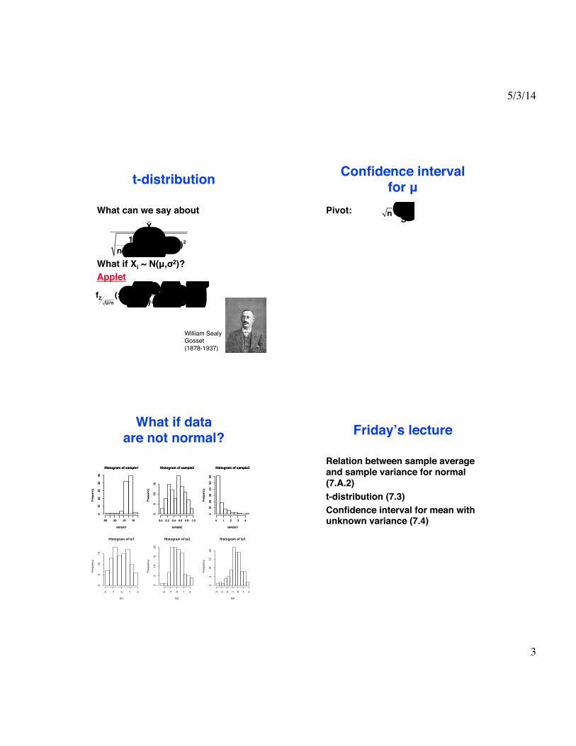
t-distribution!

What can we say about!!!!What if Xi ~ N(μ,σ2)?!Applet!

X1

n(n − 1)(Xi − X)

2

i=1

n

∑

fZU/n(x) = Γ( n+12 )

Γ( n2 ) nπ1+ x

2

n⎛⎝⎜

⎞⎠⎟

−n+12

William Sealy Gosset (1878-1937)!

Confidence interval for μ!

Pivot:! n X − µS

What if data are not normal?!

Histogram of sample1

sample1

Frequency

-50 -30 -10 10

010

2030

4050

Histogram of sample2

sample2

Frequency

0.0 0.2 0.4 0.6 0.8 1.0

05

1015

Histogram of sample3

sample3

Frequency

0 1 2 3 4

010

2030

4050

60

Histogram of sample1

sample1

Frequency

-50 -30 -10 10

010

2030

4050

Histogram of sample2

sample2

Frequency

0.0 0.2 0.4 0.6 0.8 1.0

05

1015

Histogram of sample3

sample3

Frequency

0 1 2 3 4

010

2030

4050

60

Histogram of ts1

ts1

Frequency

-2 -1 0 1 2

05

1015

Histogram of ts2

ts2

Frequency

-2 -1 0 1 2

05

1015

20

Histogram of ts3

ts3

Frequency

-4 -3 -2 -1 0 1 2

05

1015

20

Friday’s lecture!

Relation between sample average and sample variance for normal (7.A.2)!t-distribution (7.3)!Confidence interval for mean with unknown variance (7.4)!

5/3/14

4

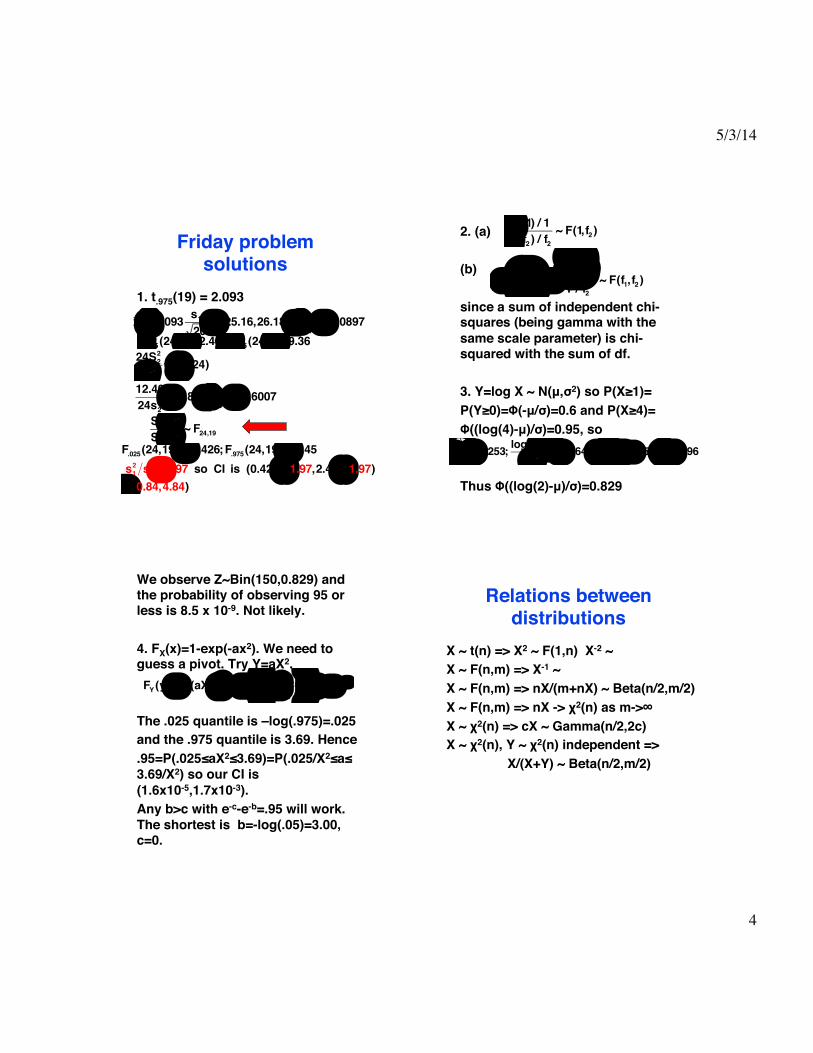
Friday problem solutions!

1. t.975(19) = 2.093!!x1 ± 2.093

s120

= (25.16,26.18)⇒ s1 = 1.0897χ.0252 (24) = 12.40; χ.975

2 (24) = 39.36

12.4024s2

2 = 0.86⇒ s22 = 0.6007

S22

S12σ12

σ22 ~ F24,19

24S22

σ22 ~ χ2(24)

F.025(24,19) = 0.426;F.975(24,19) = 2.45s12 s22 =1.97 so CI is (0.426 × 1.97,2.45 × 1.97)= (0.84,4.84)

2. (a)!!(b)!!since a sum of independent chi-squares (being gamma with the same scale parameter) is chi-squared with the sum of df. !!3. Y=log X ~ N(μ,σ2) so P(X≥1)=!P(Y≥0)=Φ(-μ/σ)=0.6 and P(X≥4)=!Φ((log(4)-μ)/σ)=0.95, so!!!Thus Φ((log(2)-μ)/σ)=0.829!

χ2(1) / 1χ2(f2 ) / f2

~ F(1,f2 )

Z = 1f1

Zi1

f1

∑ =

1f1

Xi1

f1

∑Y / f2

~ F(f1,f2 )

− µσ= 0.253; log 4 − µ

σ= 1.645⇒ µ = −.252,σ = .996

We observe Z~Bin(150,0.829) and the probability of observing 95 or less is 8.5 x 10-9. Not likely.!!4. FX(x)=1-exp(-ax2). We need to guess a pivot. Try Y=aX2. !!!The .025 quantile is –log(.975)=.025!and the .975 quantile is 3.69. Hence!.95=P(.025≤aX2≤3.69)=P(.025/X2≤a≤ 3.69/X2) so our CI is (1.6x10-5,1.7x10-3).!Any b>c with e-c-e-b=.95 will work. The shortest is b=-log(.05)=3.00, c=0.!

FY(y) = P(aX2 ≤ y) = P X ≤ y

a⎛⎝⎜

⎞⎠⎟= 1− e −y

Relations between distributions!

X ~ t(n) => X2 ~ F(1,n) X-2 ~ !X ~ F(n,m) => X-1 ~!X ~ F(n,m) => nX/(m+nX) ~ Beta(n/2,m/2)!X ~ F(n,m) => nX -> χ2(n) as m->∞!X ~ χ2(n) => cX ~ Gamma(n/2,2c)!X ~ χ2(n), Y ~ χ2(n) independent =>!

! !X/(X+Y) ~ Beta(n/2,m/2)!

5/3/14

5

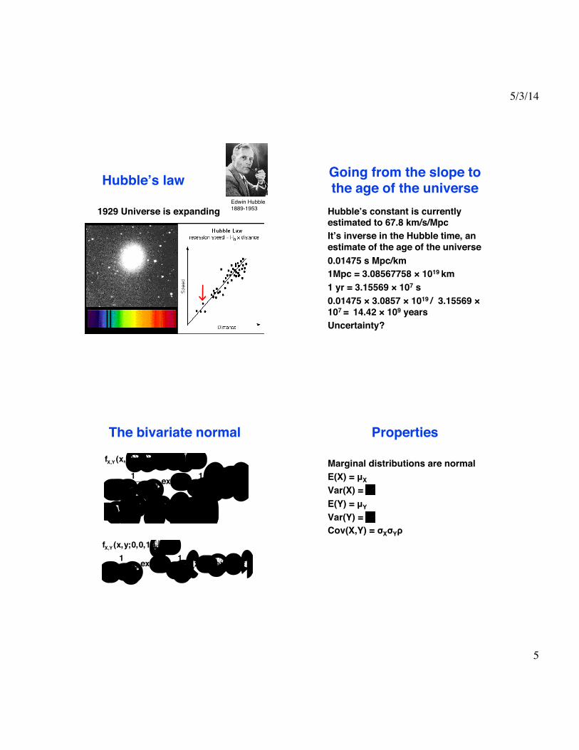
Hubble’s law !

1929 Universe is expanding!!!!!!

Edwin Hubble!1889-1953!

Going from the slope to the age of the universe!

Hubble’s constant is currently estimated to 67.8 km/s/Mpc!It’s inverse in the Hubble time, an estimate of the age of the universe!0.01475 s Mpc/km!1Mpc = 3.08567758 × 1019 km!1 yr = 3.15569 × 107 s!0.01475 × 3.0857 × 1019 / 3.15569 × 107 = 14.42 × 109 years!Uncertainty?!!

The bivariate normal!

fX,Y (x,y;µX,µY,σX2 ,σY

2 ,ρ) =

12πσXσY 1− ρ2

exp(− 12

11− ρ2

x − µX

σX

⎛⎝⎜

⎞⎠⎟

2

−2ρ x − µX

σX

y − µYσY

+ y − µYσY

⎛⎝⎜

⎞⎠⎟

2

)

fX,Y (x,y;0,0,1,1,ρ) =1

2π 1− ρ2exp(− 1

21

1− ρ2x2 − 2ρxy + y2( ))

Properties!

Marginal distributions are normal!E(X) = μX!Var(X) =!E(Y) = μY!Var(Y) =!Cov(X,Y) = σXσYρ!

σX2

σY2

5/3/14

6

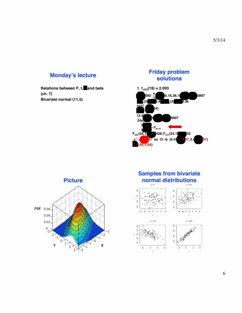
Monday’s lecture!

Relations between F, t, and beta!(ch. 7) !Bivariate normal (11.5) !

χ2

Friday problem solutions!

1. t.975(19) = 2.093!!x1 ± 2.093

s120

= (25.16,26.18)⇒ s1 = 1.0897χ.0252 (24) = 12.40; χ.975

2 (24) = 39.36

12.4024s2

2 = 0.86⇒ s22 = 0.6007

S22

S12σ12

σ22 ~ F24,19

24S22

σ22 ~ χ2(24)

F.025(24,19) = 0.426;F.975(24,19) = 2.45s12 s22 =1.97 so CI is (0.426 × 1.97,2.45 × 1.97)= (0.84,4.84)

Picture!Samples from bivariate

normal distributions!

64 66 68 70 72 74 76

130

150

170

190

x

y

ρ = 0

66 68 70 72 74 76 78

130

150

170

190

x

y

ρ = 0.5

65 70 75 80

120

140

160

180

200

x

y

ρ = -0.5

65 70 75 80

140

160

180

200

x

y

ρ = 0.95

5/3/14

7

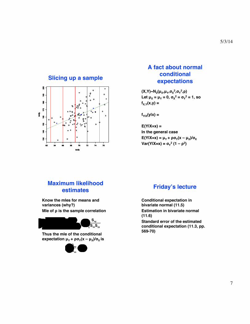
Slicing up a sample!

62 64 66 68 70 72 74 76

130

140

150

160

170

180

190

200

biv$x

biv$y

62 64 66 68 70 72 74 76

130

140

150

160

170

180

190

200

biv$x

biv$y

62 64 66 68 70 72 74 76

130

140

150

160

170

180

190

200

biv$x

biv$y

62 64 66 68 70 72 74 76

130

140

150

160

170

180

190

200

biv$x

biv$y

62 64 66 68 70 72 74 76

130

140

150

160

170

180

190

200

biv$x

biv$y

A fact about normal conditional

expectations!(X,Y)~N2(μX,μY,σX

2,σY2,ρ)!

Let μX = μY = 0, σX2 = σY

2 = 1, so!fX,Y(x,y) = !!fY|X(y|x) = !!E(Y|X=x) = !In the general case!E(Y|X=x) = μY + ρσY(x – μX)/σX!Var(Y|X=x) = σY

2 (1 – ρ2)!!

Maximum likelihood estimates!

Know the mles for means and variances (why?)!Mle of ρ is the sample correlation!!!!Thus the mle of the conditional expectation μY + ρσY(x – μX)/σX is!

ρ =(xi∑ − x)(yi − y)

(xi − x∑ )2 (yi − y)2∑=

Sxy

SxxSyy

y +Sxy

Sxx(x − x)

Friday’s lecture!

Conditional expectation in bivariate normal (11.5)!Estimation in bivariate normal (11.6)!Standard error of the estimated conditional expectation (11.3, pp.569-70)!

5/3/14

8

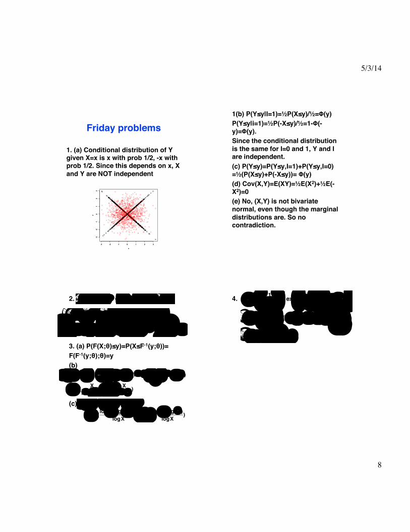
Friday problems!

1. (a) Conditional distribution of Y given X=x is x with prob 1/2, -x with prob 1/2. Since this depends on x, X and Y are NOT independent!

-3 -2 -1 0 1 2 3

-3-2

-10

12

3

x

y

-3 -2 -1 0 1 2 3

-3-2

-10

12

3

x

y

1(b) P(Y≤y|I=1)=½P(X≤y)/½=Φ(y)!P(Y≤y|i=1)=½P(-X≤y)/½=1-Φ(-y)=Φ(y).!Since the conditional distribution is the same for I=0 and 1, Y and I are independent.!(c) P(Y≤y)=P(Y≤y,I=1)+P(Y≤y,I=0) =½(P(X≤y)+P(-X≤y))= Φ(y)!(d) Cov(X,Y)=E(XY)=½E(X2)+½E(-X2)=0!(e) No, (X,Y) is not bivariate normal, even though the marginal distributions are. So no contradiction.!

2.!!!!!3. (a) P(F(X;θ)≤y)=P(X≤F-1(y;θ))=!F(F-1(y;θ);θ)=y!(b)!!!!(c) !

L(ρ) = 12π

⎛⎝

⎞⎠

n

(1− ρ2 )−n/2 exp − 12(1− ρ2 )

(xi2 − 2ρxiyi + yi2 )∑⎛⎝⎜

⎞⎠⎟

′ℓ (ρ) = nρ1− ρ2

− ρ(1− ρ2 )2

xi2 − 2ρ xiy∑ i+ yi2∑∑( )

+xiyi∑

1− ρ2= 0⇒ ρ3 − ρ2

xiyi∑n

− ρ 1−(xi2 + yi2 )∑n

⎛

⎝⎜⎞

⎠⎟−

xiyi∑n

= 0

1− α = P( α2 ≤ F(X θ) ≤ 1− α2 ) = P(F−1( α2 ) ≤

Xθ≤ F−1(1− α

2 ))

= P( XF−1(1− α

2 )≤ θ ≤ X

F−1( α2 ))

1− α = P( α2 ≤ 1− e −Xθ

≤ 1− α2 )

= P(log(− log(1−α2 ))

logX≤ θ ≤ log(− log(

α2 ))

logX)

4. !

L(α) = 12πσ2

⎛⎝

⎞⎠

n/2

exp − 12σ2 (yi − αxi)2∑⎛

⎝⎞⎠

′ℓ (α) = 1σ2 xi(∑ yi − αxi) = 0⇒ α =

xiyi∑xi2∑

′′ℓ (α) = − 1σ2 xi2∑ < 0

5/3/14

9

Standard error of the conditional expectation!Yi are random, xi are fixed.!SYx is independent of!Thus the variance is!!!!Slope?!Intercept?!Variance?!!

Y

σY2

n+ (x − x)

2

Sxx2 (xi − x)2Var(Yi)∑ = σY

2 1n+ (x − x)

2

Sxx

⎛⎝⎜

⎞⎠⎟

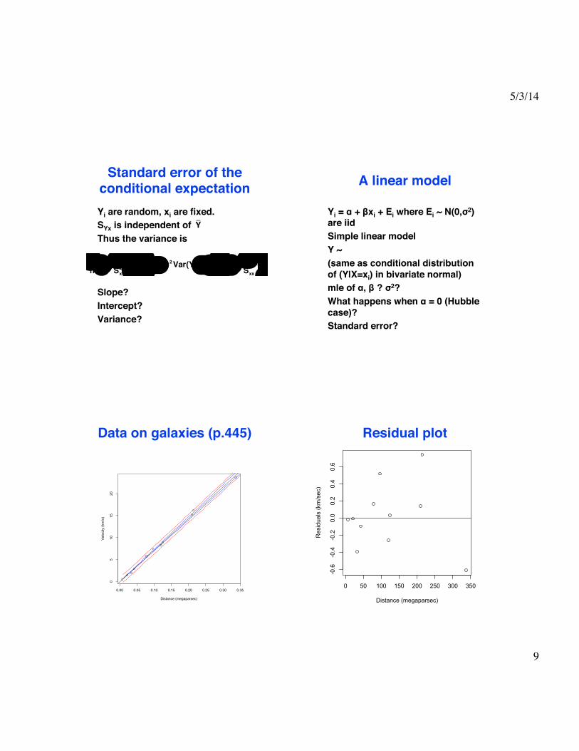
A linear model!

Yi = α + βxi + Ei where Ei ~ N(0,σ2) are iid!Simple linear model!Y ~ !(same as conditional distribution of (Y|X=xi) in bivariate normal)!mle of α, β ? σ2?!What happens when α = 0 (Hubble case)?!Standard error?!

Data on galaxies (p.445)!

0.00 0.05 0.10 0.15 0.20 0.25 0.30 0.35

05

1015

20

Distance (megaparsec)

Vel

ocity

(km

/s)

Residual plot!

0 50 100 150 200 250 300 350

-0.6

-0.4

-0.2

0.0

0.2

0.4

0.6

Distance (megaparsec)

Res

idua

ls (k

m/s

ec)

5/3/14

10

Sum of squares!Let ! ! ! !and write!

! ! ! . Squaring both sides and summing we get !!Now, the second term is!!so the first must be !We write this decomposition!SSTot = SSRes + SSModel!!

yi = y + β(xi − x)yi − y = yi − yi + yi − y

(yi − y)2 = (yi − yi )

2 + (∑∑∑ yi − y)2

β2 (xi∑ − x)2 = Sxy2 Sxx = Syy ρ

2

Syy(1− ρ2 )

SSTot ~ σ2χ2(n − 1)SSRes ~ σ2χ2(n − 2)SSmodel ~ σ2χ2(1)

⎫⎬⎭independent

Monday’s lecture!

The simple linear model!Estimating the age of the universe!Decomposing the sum of squares!

Confidence bands and tests!

Slope:!!!!!!!Regression:!!

β =(xi − x)(Yi − Y)∑(xi − x)2∑

~ N(β, σ2

(xi − x)2∑)

!σ2 = SSRes / (n − 2)

β − β!σ2 / Sxx

~

SSModel 1SSRes n − 2

∼F1,n−2

What if we drop the normal assumption?!

Yi = α + βxi + Ei where Ei have mean zero, variance σ2, and are uncorrelated.!No likelihood theory available!Method of least squares (Legendre, 1805)!

Adrien-Marie!Legendre!1752-1833!

5/3/14

11

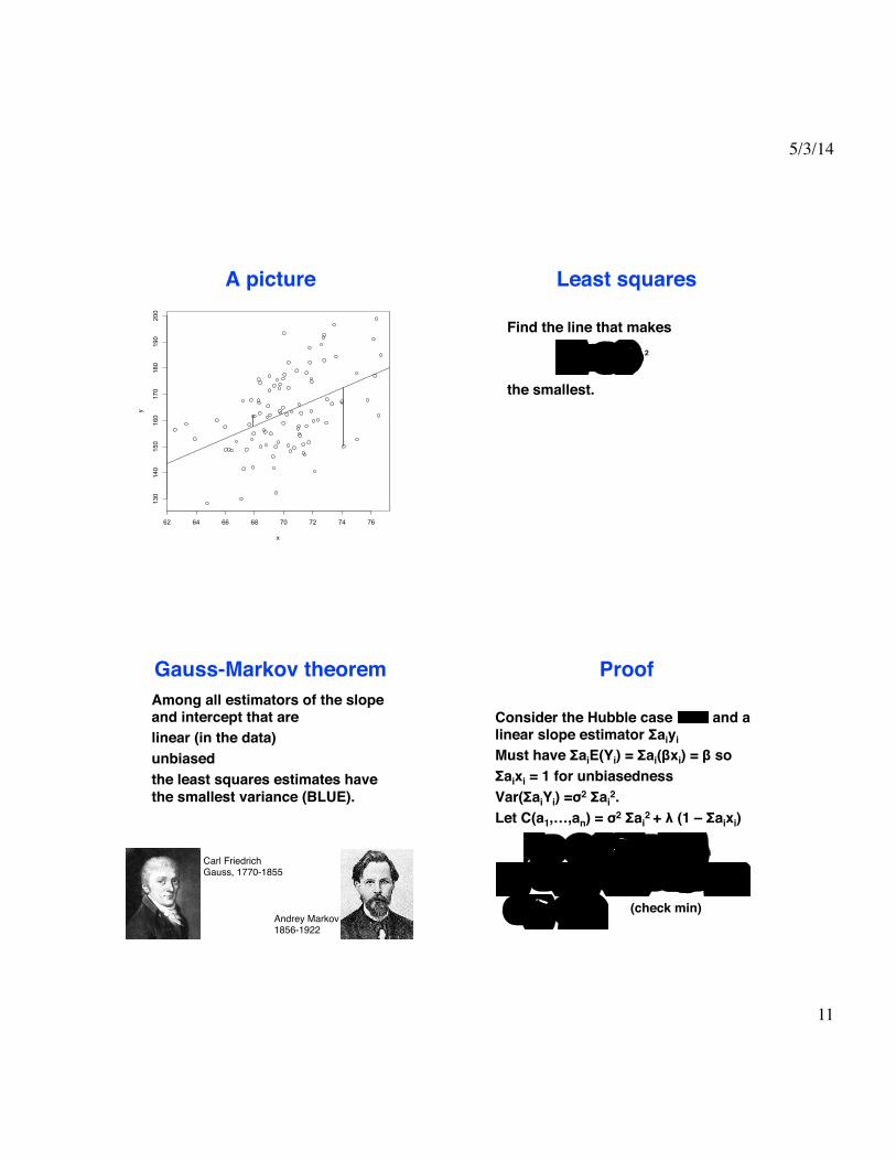
A picture!

!!

62 64 66 68 70 72 74 76

130

140

150

160

170

180

190

200

x

y

Least squares!

Find the line that makes!!!the smallest.!

(yii=1

n

∑ − α − βxi)2

Gauss-Markov theorem!Among all estimators of the slope and intercept that are!linear (in the data)!unbiased!the least squares estimates have the smallest variance (BLUE).!

Carl Friedrich!Gauss, 1770-1855!

Andrey Markov!1856-1922!

Proof!

Consider the Hubble case and a linear slope estimator Σaiyi!Must have ΣaiE(Yi) = Σai(βxi) = β so !Σaixi = 1 for unbiasedness!Var(ΣaiYi) =σ2 Σai

2.!Let C(a1,…,an) = σ2 Σai

2 + λ (1 – Σaixi)!! ∂C

∂ai= 2aiσ2 − λxi;

∂C∂λ

= 1− aixi∑

∂C∂ai

∑ xi = 2σ2 aixi∑1

!"#− λ xi2∑ = 0⇒ λ = 2σ2 1

xi2∑ai =

λ2σ2 xi =

xixi2∑

(check min)!

α = 0

5/3/14

12

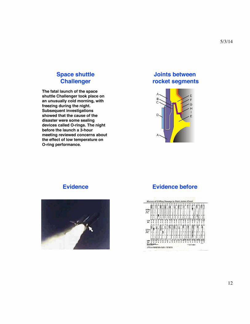
Space shuttle Challenger!

The fatal launch of the space shuttle Challenger took place on an unusually cold morning, with freezing during the night. Subsequent investigations showed that the cause of the disaster were some sealing devices called O-rings. The night before the launch a 3-hour meeting reviewed concerns about the effect of low temperature on O-ring performance. !!

Joints between rocket segments!

Evidence! Evidence before!

5/3/14

13

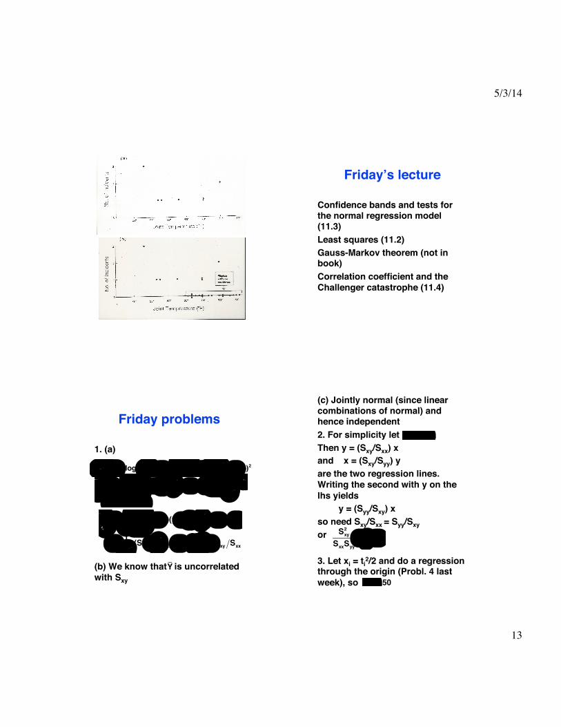
Friday’s lecture!

Confidence bands and tests for the normal regression model (11.3)!Least squares (11.2)!Gauss-Markov theorem (not in book)!Correlation coefficient and the Challenger catastrophe (11.4)!

Friday problems!

1. (a)!!!!!!!!!(b) We know that is uncorrelated with Sxy !!!!!! !

ℓ(α,β) = n

2log(2πσ2 ) − 1

2σ2 (yi − α − β(xi − x))2∑

∂ℓ∂α

= 12σ2 (yi − α∑ − β(xi − x) =

yi − nα∑2σ2

= 0⇔ α = y

∂ℓ∂β

= 12σ2 (xi − x)(yi − α∑ − β(xi − x)) =

= 12σ2 (Sxy − βSxx ) = 0⇔ β = Sxy Sxx

Y

(c) Jointly normal (since linear combinations of normal) and hence independent!2. For simplicity let!Then y = (Sxy/Sxx) x !and x = (Sxy/Syy) y !are the two regression lines. Writing the second with y on the lhs yields !

!y = (Syy/Sxy) x!so need Sxy/Sxx = Syy/Sxy!or!!3. Let xi = ti

2/2 and do a regression through the origin (Probl. 4 last week), so !

x = y = 0.

Sxy2

SxxSyy= ρ2 = 1

a = 0.50

5/3/14

14

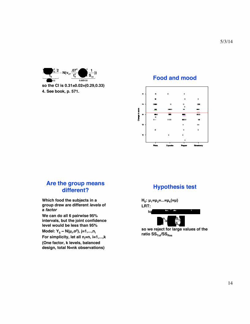
!!so the CI is 0.31±0.02=(0.29,0.33)!4. See book, p. 571.!

Y0 − a t02 2t0

v0=0.313! "# $#

∼N(v0,.072

t02(1+ t0

4

41Sxx

)

0.000133! "## $##

)Food and mood!

Cha

nge

in s

core

Pizza Cupcake Pepper Strawberry-4

-20

24

Cha

nge

in s

core

Pizza Cupcake Pepper Strawberry-4

-20

24

Cha

nge

in s

core

Pizza Cupcake Pepper Strawberry-4

-20

24

Cha

nge

in s

core

Pizza Cupcake Pepper Strawberry-4

-20

24

Cha

nge

in s

core

Pizza Cupcake Pepper Strawberry-4

-20

24

Cha

nge

in s

core

Pizza Cupcake Pepper Strawberry-4

-20

24

Are the group means different?!

Which food the subjects in a group drew are different levels of a factor!We can do all 6 pairwise 95% intervals, but the joint confidence level would be less than 95%!Model: Yij ~ N(μi,σ2), j=1,...,ni!For simplicity, let all ni=n, i=1,...,k!(One factor, k levels, balanced design, total N=nk observations)!

Hypothesis test!

H0: μ1=μ2=...=μk(=μ)!LRT:!!!!so we reject for large values of the ratio SSTot/SSRes!!

log(Λ) = ℓ(µ1,..., µk; σA2 ) − ℓ(µ; σ0

2 )

= kn2log SSTot

SSRes⎛⎝⎜

⎞⎠⎟

5/3/14

15

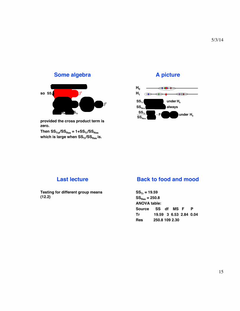
Some algebra!

!so!!!!!provided the cross product term is zero.!Then SSTot/SSRes = 1+SSTr/SSRes!which is large when SSTr/SSRes is. !!

Yij − Yii = Yij − Yii + Yii − Yii

SSTot = (Yij − Yii )2j=1

N

∑i=1

N

∑

= (Yij − Yii )2j=1

n

∑i=1

k

∑ + ni(Yii − Yii )2i=1

k

∑= SSRes + SSTr

A picture!

H0!H1!

SSTr ∼ σ2χ2(k − 1) under H0

SSRes ∼ σ2χ2(N − k) always

SSTr k − 1SSRes N − k

∼F(k − 1,N − k)under H0

Last lecture!

Testing for different group means (12.2)!

Back to food and mood!

SSTr = 19.59!SSRes = 250.8!ANOVA table:!Source SS df MS F P!Tr ! !19.59 3 6.53 2.84 0.04!Res ! 250.8 109 2.30!

5/3/14

16

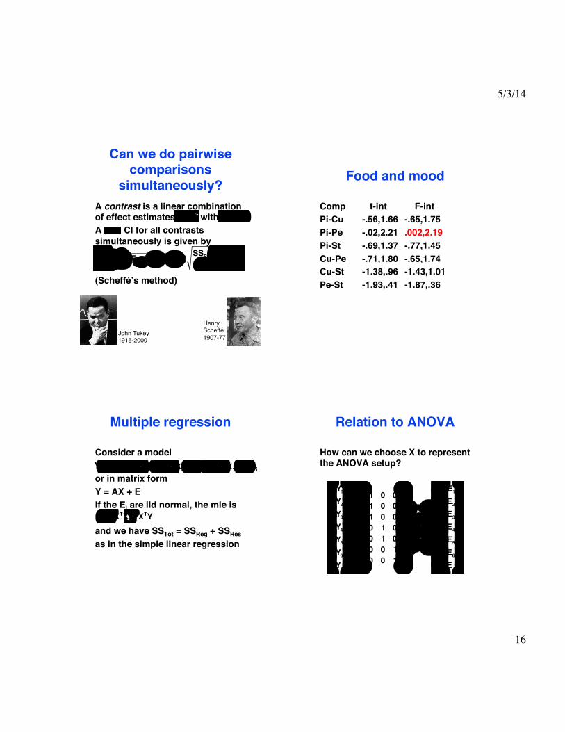
Can we do pairwise comparisons

simultaneously?!A contrast is a linear combination of effect estimates with!A ! CI for all contrasts simultaneously is given by!!!(Scheffé’s method)!!

Henry Scheffé!1907-77!

ciµ i∑ ci = 0.∑1− α

ciµ i ± F1−α (k − 1,N − k∑ ) SSResN − k

ci2

ni∑⎛⎝⎜

⎞⎠⎟

John Tukey!1915-2000!

Food and mood!

Comp ! t-int ! F-int!Pi-Cu !-.56,1.66 !-.65,1.75!Pi-Pe !-.02,2.21 !.002,2.19!Pi-St! !-.69,1.37 !-.77,1.45!Cu-Pe !-.71,1.80 !-.65,1.74!Cu-St !-1.38,.96 !-1.43,1.01!Pe-St !-1.93,.41 !-1.87,.36!

Multiple regression!

Consider a model!!or in matrix form!Y = AX + E!If the Ei are iid normal, the mle is!!and we have SSTot = SSReg + SSRes!as in the simple linear regression!

Yi = α0 + α1xi1 + α2xi2 +!+ αpx1p +Ei

A = XTX( )−1XTY

Relation to ANOVA!

How can we choose X to represent the ANOVA setup?!

Y1Y2Y3Y4Y5Y6Y7

⎡

⎣

⎢⎢⎢⎢⎢⎢⎢⎢⎢

⎤

⎦

⎥⎥⎥⎥⎥⎥⎥⎥⎥

=

1 0 01 0 01 0 00 1 00 1 00 0 10 0 1

⎡

⎣

⎢⎢⎢⎢⎢⎢⎢⎢

⎤

⎦

⎥⎥⎥⎥⎥⎥⎥⎥

µ1µ2µ3

⎡

⎣

⎢⎢⎢

⎤

⎦

⎥⎥⎥+

E1E2E3E4E5E6E7

⎡

⎣

⎢⎢⎢⎢⎢⎢⎢⎢⎢

⎤

⎦

⎥⎥⎥⎥⎥⎥⎥⎥⎥

5/3/14

17

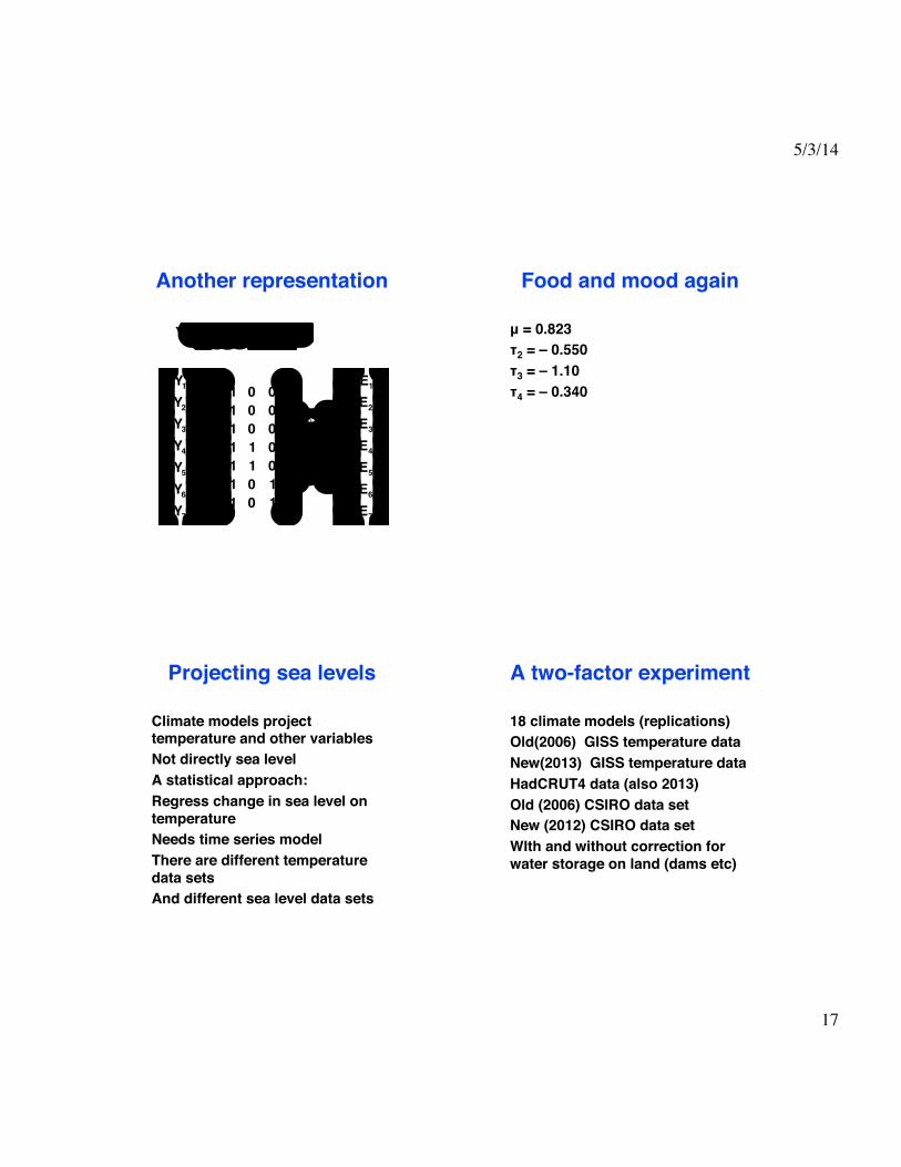
Another representation!

Y1Y2Y3Y4Y5Y6Y7

⎡

⎣

⎢⎢⎢⎢⎢⎢⎢⎢⎢

⎤

⎦

⎥⎥⎥⎥⎥⎥⎥⎥⎥

=

1 0 01 0 01 0 01 1 01 1 01 0 11 0 1

⎡

⎣

⎢⎢⎢⎢⎢⎢⎢⎢

⎤

⎦

⎥⎥⎥⎥⎥⎥⎥⎥

µτ2τ3

⎡

⎣

⎢⎢⎢

⎤

⎦

⎥⎥⎥+

E1E2E3E4E5E6E7

⎡

⎣

⎢⎢⎢⎢⎢⎢⎢⎢⎢

⎤

⎦

⎥⎥⎥⎥⎥⎥⎥⎥⎥

Yij = µ + τi +Eij, τii∑ = 0

Food and mood again!

μ = 0.823!τ2 = – 0.550!τ3 = – 1.10!τ4 = – 0.340!

Projecting sea levels!

Climate models project temperature and other variables!Not directly sea level!A statistical approach:!Regress change in sea level on temperature!Needs time series model!There are different temperature data sets!And different sea level data sets!

A two-factor experiment!

18 climate models (replications)!Old(2006) GISS temperature data!New(2013) GISS temperature data!HadCRUT4 data (also 2013)!Old (2006) CSIRO data set!New (2012) CSIRO data set!WIth and without correction for water storage on land (dams etc)!

5/3/14

18

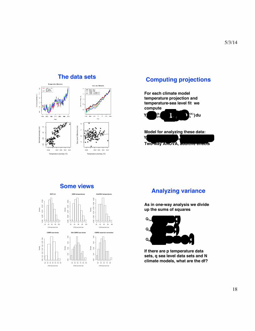
The data sets!

●●

●●

●●●● ● ●● ●●

●

●

●●●

●●

●●●

●

●●●●●

●●●●●

●●●

● ●●●●●●

●●●●

●●● ●●

●●

●●

●●●

●

●●●●●

●●●●●● ●

●●●●

●●●●

●●●

●

●●●●

●●●

●●

● ●● ●●

●●

●●

●●

● ● ●●

● ●●●● ●

●●●

●●

−0.6 −0.2 0.0 0.2 0.4

−15

−10

−50

(a)

Temperature anomaly (°C)

Sea

leve

l ano

mal

y (c

m)

●

●

●

●

●●

●

● ●●

●

●●

●

●

●

●

●●

●

●

●

●

●

●

●

●●

●

●

●

●

●

●●

●

●

●

●●●

●

●

●

●

●

●

●

●

●

●

●●

●

●

●

●

●

●

●

●

●●

●

●

●

●●

●

●

●

●

●

●

●

●

●

●●

●

●

●

●

●

●

●

●●

●

●

●

●

●

●

●● ●

●

●

●

●

●

●

●

●

● ●

●●

●●●

●

●●

●

●

●

●

−0.6 −0.2 0.0 0.2 0.4

−10

12

(c)

Temperature anomaly (°C)

Sea

Leve

l Diff

eren

ce (c

m)

1880 1920 1960 2000

−6−4

−20

24

6

(b)

Year

Res

idua

l (cm

)

1880 1920 1960 2000

−10

12

(d)

Year

Res

idua

l (cm

)

1880 1920 1960 2000

−1.5

−0.5

0.5

1.0

1.5

(e)

Year

Inno

vatio

n (c

m)

Computing projections!

For each climate model temperature projection and temperature-sea level fit we compute!!!!Model for analyzing these data:!!Two-way ANOVA, additive effects!

Yijk = H2100

ijk = (⌢γ ij + δ ijTu(k) )du2000

2100

∫

Yijk = µ + α i + β j +Eijk α ii∑ = β j = 0

j∑

Some views!RCP 2.8

2100 sea level rise

Density

20 40 60 80 100

0.000

0.005

0.010

0.015

0.020

GISS temperatures

2100 sea level rise

Density

20 40 60 80 100

0.000

0.005

0.010

0.015

0.020

HadCRU temperatures

2100 sea level rise

Density

20 40 60 80 100

0.000

0.005

0.010

0.015

0.020

0.025

CSIRO sea levels

2100 sea level rise

Density

25 30 35 40 45 50 55

0.00

0.01

0.02

0.03

0.04

0.05

0.06

Old CSIRO sea levels

2100 sea level rise

Density

40 50 60 70 80 90

0.00

0.01

0.02

0.03

0.04

CSIRO reservoir correction

2100 sea level rise

Density

40 50 60 70 80

0.00

0.01

0.02

0.03

0.04

Analyzing variance!

As in one-way analysis we divide up the sums of squares!!!!!!!If there are p temperature data sets, q sea level data sets and N climate models, what are the df?!

QTemp = Yiii − Yiii( )i,j,k∑ 2

QSeal = Yi ji − Yiii( )i,j,k∑ 2

QRes = Yiji − Yiii − Yi ji + Yiii( )i,j,k∑ 2

5/3/14

19

ANOVA table!

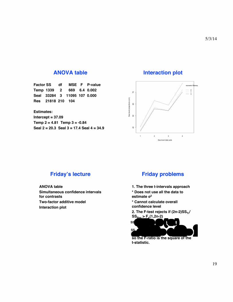
Factor SS df !MSE! F ! P-value!Temp 1339 !2 !669 ! 6.4 ! 0.002!Seal! 33284 !3 11095 107 0.000!Res ! 21818 210 104 !!!Estimates:!Intercept = 37.09!Temp 2 = !4.81 Temp 3 = -0.84!Seal 2 = 20.3 Seal 3 = 17.4 Seal 4 = 34.9!

Interaction plot!

4050

6070

Sea level data sets

Sea

leve

l pro

ject

ions

(cm

)

1 2 3 4

scenario1$temp

213

Friday’s lecture!

ANOVA table!Simultaneous confidence intervals for contrasts!Two-factor additive model!Interaction plot!

Friday problems!

1. The three t-intervals approach!* Does not use all the data to estimate σ2!* Cannot calculate overall confidence level!2. The F-test rejects if (2n-2)SSTr/SSRes > Fα(1,2n-2)!!!!so the F-ratio is the square of the t-statistic.!!

SSTr = n (Yii − Yii )2

i=1

2

∑ = 12n Y1i − Y2i( )2

SSRes2n − 2

= 12

1n − 1

(Y1j − Y1i )2

j=1

n

∑ + 1n − 1

(Y2j − Y2i )2

j=1

n

∑⎛

⎝⎜⎞

⎠⎟

5/3/14

20

3. (a) GLRT is!!!where!!!!Now!and independent of so our F-test rejects when !!!(b) The difference from the one-factor ANOVA derived in class is !

log(Λ) = ℓ(µ1,..., µk; σA2 ) − ℓ(0; σ0

2 )= c − N

2 log(σA2 σ0

2 )

σA2 = 1

N(Yij − Yii )

2

j=1

ni

∑i=1

k

∑ ~ σ2

Nχ2(N − k)

σ02 = 1

NYij2

jk∑ ~ σ2

Nχ2(N)

σ02 − σA

2 = niN∑ Yii

2 ~ σ2

Nχ2(k)

σA2

ni∑ Yii(Yij − Yii )∑∑

> Fα (k,N − k)

that the variance is known, so our test needs not standardize by an estimate of σ2. Instead we use that!!so we reject when!4. Since!we have!!!!yielding !

SSTr ∼ χ2(k − 1) under H0

SSTr > χα2 (k − 1)

SSRes ∼ σ2χ2(N − k)

1− α = P(χα /22 (N − k) ≤ SSRes

σ2 ≤ χ1−α /22 (N − k))

= P( SSResχ1−α /22 (N − k)

≤ σ2 ≤ SSResχα /22 (N − k)

)

5.4123.34

, 5.414.40

⎛⎝

⎞⎠ = (0.23,1.23)

Review!

Independence of sample average and sample variance for normal !Chi-square, F and t!Confidence intervals for normal!

Mean with unknown variance!Variance!Ratio of variances!

Bivariate normal distribution!Conditional normal distribution!Estimation in bivariate normal!SE of estimated conditional expectation!!!!!

Standard error of slope!Simple linear model!Decomposing the sum of squares!Confidence bands and tests!Least squares!Gauss-Markov theorem!Testing for different group means!Decomposing the sum of squares!ANOVA table!Simultaneous confidence intervals for contrasts!Two-factor additive model!Interaction plot!!!!!!!!