OXYGEN ISOTOPES IN FORAMINIFERA: OVERVIEW …orca.cf.ac.uk/41988/1/Pearson 2012 Oxygen isotope...

OXYGEN ISOTOPES IN FORAMINIFERA: OVERVIEW AND HISTORICAL REVIEW

PAUL N. PEARSON

School of Earth and Ocean Sciences, Main Building, Cardiff University, Park Place, Cardiff, CF10 3AT, United Kingdom

[email protected]

ABSTRACT.—Foraminiferal tests are a common component of many marine sediments. The oxygen iso-tope ratio (δ18O) of test calcite is frequently used to reconstruct aspects of their life environment. The δ18O depends mainly on the isotope ratio of the water it is precipitated from, the temperature of calcifica-tion, and, to a lesser extent, the carbonate ion concentration. Foraminifera and other organisms can poten-tially preserve their original isotope ratio for many millions of years, although diagenetic processes can alter the ratios. Work on oxygen isotope ratios of foraminifera was instrumental in the discovery of the orbital theory of the ice ages and continues to be widely used in the study of rapid climate change. Com-pilations of deep sea benthic foraminifer oxygen isotopes have revealed the long history of global climate change over the past 100 million years. Planktonic foraminifer oxygen isotopes are used to investigate the history of past sea surface temperatures, revealing the extent of past 'greenhouse' warming and global sea surface temperatures.

INTRODUCTION

THE MEASUREMENT of oxygen isotope ratios of biogenic calcite is one of the longest-established and most widely used of all paleocli-mate proxies. It principally provides information on the temperature or oxygen isotope ratio of seawater at the time of calcification if the other parameter is known or assumed. The signal can, in principle, survive for hundreds of millions of years in fossils. Although many types of organ-isms produce calcite skeletons, foraminifera have been employed particularly widely because of their abundance and diversity in marine sediment, especially deep-sea oozes where many of the longest and most continuous paleoclimate records are found. Here, the development of the proxy in both benthic and planktonic foraminifera is re-viewed in two parts. Part 1 is an overview of the principles of the technique and its early develop-ment, together with some of its complications and limitations. Part 2 outlines some of the major ap-plications in paleoclimate studies from the 1970s to the present.

PART 1: PRINCIPLES AND HISTORY

Oxygen isotopes

Note: A number of textbooks provide succinct accounts of oxygen isotope systematics and measurement; this section is based mainly on Faure and Mensing (2005), Allègre (2008), and Hoefs (2009). Oxygen has three stable isotopes, 16O, 17O, and 18O, which occur on Earth in the approximate proportions 99.757%, 0.038%, and 0.205%, re-spectively (Rosman and Taylor, 1998; other sources give slightly different figures). These dif-ferent abundances reflect the fact that the three isotopes are produced by different synthetic path-ways in stars. The proportions vary somewhat in natural Earth materials because each substance has its own prior history of fractionation (proc-esses that sorted or partitioned the isotopes) and mixing (processes that combined or assimilated the isotopes). Fractionations occur in two main ways, isotope-exchange reactions and kinetic ef-fects. Because molecules with a heavy isotope have slightly greater covalent bond strengths and lower vibrational frequencies than their lighter counterparts, they are slightly less reactive. They are also slower to diffuse along concentration gradients and across membranes. Examples of fractionation processes that affect oxygen isotopes in water are evaporation, in which the light iso-tope 16O is slightly preferred, and condensation,

In Reconstructing Earth’s Deep-Time Climate—The State of the Art in 2012, Paleontological Society Short Course, November 3, 2012. The Paleontological Society Papers, Volume 18, Linda C. Ivany and Brian T. Huber (eds.), pp. 1–38. Copyright © 2012 The Paleontological Society.

where the heavy isotope 18O is slightly preferred. The physical mixing of two water masses with different isotopic ratios (e.g. when a river flows into the sea) will produce water with an interme-diate ratio. Because most natural fractionation and mix-ing processes are strictly mass dependent, the iso-topes 17O and 18O fractionate and combine rela-tive to 16O proportionally according to their re-spective masses (18O fractionating twice as much as 17O), so for most applications, there is little to be gained by measuring both isotopes. The normal procedure is to measure the ratio of 18O to 16O in a sample. By convention, the isotope ratio, R, is defined as the abundance of the heavier isotope over the abundance of the lighter isotope. For the global average proportions given above, this is expressed as follows:

R = = = 0.002055 18O16O

0.205

99.757

Because natural fractionations are, in practice, quite small, and 18O is always very much rarer than 16O, the isotopic ratios of natural materials are generally quite close to this average value. Small differences between small numbers are un-wieldy, so (as is the convention for other stable isotope systems) oxygen isotope ratios are gener-ally quoted as deviations (delta values) from the oxygen isotope ratio (δ18O) of a standard sub-stance in parts per thousand ('per mil', sometimes ‘per mille’, signified by the symbol, ‘‰’).

δ18O = x 1000 Rsample - Rstandard

Rstandard

There are also good, practical reasons for this convention because isotope ratios of sample mate-rials are almost always measured relative to a laboratory standard rather than as an absolute ra-tio, which is much more difficult to determine accurately. Note that if a sample has a positive δ18O, it is said to be enriched in the heavy isotope relative to the standard and, if negative, it is said to be depleted. It so happens that two different standard val-ues are in widespread use from which these delta-values are quoted: Vienna Standard Mean Ocean Water (VSMOW) and Vienna Pee Dee Belemnite (VPDB, which is a carbonate standard; the his-

torical reason for the adoption of this is described below). The original standards were simply SMOW and PDB, but because original supplies of both standards ran out and some inter-laboratory differences emerged in defining what the precise values were relative to other available reference materials, a worldwide convention was deter-mined (at a meeting in Vienna) (Gonfiantini, 1984; see Coplen, 1994, for further discussion). Deviations from VSMOW tend to be used in stud-ies of the hydrological cycle and also for high-temperature processes, such as in metamorphic rocks, and studies of phosphates and silica. Devia-tions from VPDB tend to be used in studies of low-temperature carbonates, including foramini-fera. Note that carbon isotope ratios in carbonates, 13C/12C, are also quoted relative to the same VPBD standard (as δ13C ‰). The oxygen isotope ratios of carbonate sam-ples are usually measured using a gas source mass spectrometer. The sample is reacted with 100% phosphoric acid, producing CO2 gas that is ion-ized in a vacuum chamber by electron bombard-ment. The mass spectrometer accelerates the ions under high voltage, and a magnetic field splits them into streams of different isotope ratio that generate electrical currents in the detectors. The ratio of these currents is proportional to the iso-tope ratio of the sample. By alternately switching between a standard of known isotope ratio (gener-ally a CO2 reference gas supplied by the National Institute of Standards and Technology) and an unknown sample, the isotope ratio of the un-known can be calculated. In this way, the follow-ing masses are usually measured: 12C16O16O (mass 44), 13C16O16O (mass 45), and 12C18O16O (mass 46) (higher masses are created from other combinations of 13C and 18O, but these are rare and not routinely measured). From these ratios, the δ18O and δ13C of the sample are calculated simultaneously and quoted relative to VPDB. In reality, some complications have to be taken into account, notably subtraction of the contribution of molecules containing 17O to the above masses, and the effect of isotopic fractionation associated with the phosphoric acid reaction.

Foraminiferal calcite Foraminifera are single-celled eukaryotic or-ganisms belonging to the Phylum Granuloreticu-losa, which comprises amoeboid organisms char-acterized by pseudopodia that have a granular texture to the flowing cytoplasm (Lee et al.,

THE PALEONTOLOGICAL SOCIETY PAPERS, VOL. 18

2

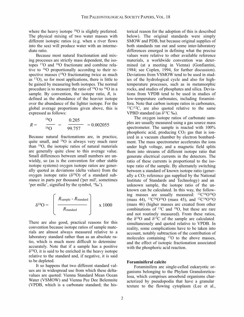
2000). Most foraminifera are marine, and many secrete a test (or shell) made of calcium carbonate (CaCO3; generally low-Mg calcite, but high-Mg calcite in porcelaneous species and aragonite in some groups). Some foraminifera live among the ocean plankton distributed in the upper part of the water column; others are benthic, living directly on the sea floor or at shallow depths in the sedi-ment (Figure 1). Foraminifera are heterotrophs, feeding on organic matter rather than photosyn-thesizing, although many species live in symbiotic association with photosynthetic algae. Foraminif-eral tests can occur in large numbers, and in many places, they form a significant component of the sea-floor sediment (for quantitative estimates, see Schiebel, 2002). The oxygen in foraminiferal cal-cite derives from the seawater (or, in the case of infaunal species, the pore water) in which the or-ganism lived. Hence, the isotope ratios can pro-vide information about the composition and his-tory of that water, and the environmental condi-tions in which the test was secreted. Most foraminiferal tests are built from suc-

cessive chambers added episodically throughout life, starting with a first-formed chamber (prolo-culus). The chambers all have small openings or foramina (singular: foramen) that provide internal connections between them and allow cytoplasm flow inside and outside the test (hence 'foramini-fera', which means 'bearers of foramina'). Gener-ally, the chambers increase in size through the life cycle (ontogeny). Different groups of foraminifera have adopted a wide variety of chamber shapes and geometries of chamber addition, with spiral arrangements being the most common. This means that many types of foraminifera can be readily distinguished by eye (Figure 1). Foramini-fer tests are large enough (mostly in the range 0.1–1.0 mm) that they can be manually separated (picked) under a binocular microscope with a fine brush or needle, and their isotopic ratios can be determined either individually or by combining relatively small numbers of tests of the same spe-cies. This is a convenient advantage in paleocli-mate research over smaller biogenic particles such as coccoliths, which are also very common in ma-

PEARSON: OXYGEN ISOTOPES IN FORAMINIFERA

FIGURE 1.—Foram art: calcite tests of selected benthic (left) and planktonic (right) foraminifera. These are from exceptionally well-preserved Paleogene sediments of Tanzania (33–45 Ma). Scale is approximate; diameters are from about 0.20–0.75 mm. Images: P. N. Pearson and I. K. McMillan. Note the literature is split between those who use the adjective 'planktonic' versus 'planktic' and between those who use 'benthonic' versus 'benthic'. It so happens that planktonic and benthic are clearly in the ascendancy as of 2012, by roughly 10:1 and 30:1 respectively, as shown by a word search on abstracts. It has been argued that planktic is the correct Greek form of the adjective (Rodhe, 1974; Emiliani, 1991) but it has been pointed out that planktonic, like electronic, is perfectly good English, however ugly it may be in Greek (Hutchinson, 1974). The majority usage is followed here.

3

rine carbonates, but cannot easily be separated into species, and are too small to analyze indi-vidually. Foraminiferal life cycles generally last weeks or months, although there is evidence that some of very large (> 1 cm) benthic species of the past may have lived for several years (Purton and Brasier, 1999). The complex process of test secre-tion (biomineralization) has been studied for many living species, both benthic (Erez, 2003) and planktonic (Hemleben et al., 1989). The de-tails vary across the biological subgroups, as do the distinctive test microstructures that result. Chamber formation is always episodic with a pe-riod of rest and feeding in between. The solid chambers are constructed in a matter of hours from many millions of minute calcite plaques, or microgranules, which themselves are formed in-tracellularly (Hemleben et al., 1989). In some species, seawater is vacuolated and transported inside the cell (Bentov et al., 2009). The vacuole in which the calcite is precipitated is separated from both seawater and cytoplasm by membranes (Erez, 2003). The chamber itself is formed on an organic template, and an organic membrane is found within the test wall of most species. The temperature within the cell is set by ambient conditions, but the observed rates of cal-cification are at least an order of magnitude slower than inorganic precipitation (Erez, 2003). Because the formation of calcite is so clearly bio-logically mediated, there is considerable potential for biological fractionation of the various isotopes and trace metals incorporated into the calcite (see Zeebe et al., 2008, for a review). Despite this, foraminifera have been found to secrete calcium carbonate close to isotopic equilibrium, unlike certain other types of calcifiers such as corals, echinoderms, and arthropods (Wefer and Berger, 1991). However, small but significant disequilib-rium effects (sometimes called vital effects) have been reported and are discussed further below.

The heroic age of oxygen isotopes As mentioned above, a molecule with a heavy isotope has a slightly greater covalent bond strength and a lower vibrational frequency than its lighter counterpart so it is slightly less reactive. This difference in reactivity is influenced by the ambient temperature such that an increase in tem-perature lessens the difference in reaction rates (essentially, this is because everything vibrates faster at higher temperature). The idea that this effect could be exploited by measuring the oxy-

gen isotope ratio of a calcite shell to determine its temperature of calcification dates back to the work of Harold Urey and colleagues (Urey, 1947, 1948; the latter paper reports results of collabora-tive work between himself, Charles McKinney, John McCrea, and Samuel Epstein at the Univer-sity of Chicago; see also Epstein, 1997, for a per-sonal account of the period). Urey (1947) began his investigation by making calculations of the isotope exchange reaction between water and car-bonate ions. As he himself explained: “If calcium carbonate is crystallized slowly in the presence of water at 0°C, the calculations show that the ratio of the oxygen isotopes in the calcium carbonate should be 1.026 to 500 if the ratio of the isotopes in the water is 1 to 500, i.e. oxygen 18 is very slightly concentrated in the calcium carbonate in relation to the water. On the other hand, if the temperature is 25°C, the oxygen isotopes will be concentrated only to the extent of 1.022 as com-pared with 1 in 500 on water. This shows that there is a slight temperature coefficient for the abundance of 18O isotope in the calcium carbon-ate.” (Urey, 1948, p. 491; note that these figures would now be revised somewhat.) Urey (1948) pointed out that these differ-ences, although small, were measurable and con-sistent with the actual isotopic ratios of a variety of biogenic carbonates that he and his colleagues measured to investigate the effect. They did this on a pioneering mass spectrometer built to the design of Alfred Nier (see Nier, 1947, and McKinney et al., 1950, for early analytical devel-opments). Among the carbonates measured were two samples of Globigerina ooze from the Pacific Ocean at 60°S. Globigerina is a genus of plank-tonic foraminifer, hence, these were the first of the very many foraminifera to be dissolved and analyzed in the pursuit of temperature informa-tion. The δ18O values of these samples were re-ported as +2.14 and +1.85 relative to a mollusk that grew at 13°C (note the PDB standard had yet to be defined). These enriched isotope ratios im-plied a cooler calcification temperature for the foraminifera than the mollusk, which was consis-tent with the high-latitude location. “I suddenly found myself with a geologic thermometer in my hands,” Urey is reported to have said (Emiliani, 1958, p. 2). Although he also admitted it was "not useful" (Epstein, 1997, p. 8), it was evidently an interesting problem and, in the immediate post-war period, a welcome non-military application of isotope physics. Urey (1948) reported measure-ments of a variety of samples from the Cretaceous


4

chalk of England to underline his point, estimat-ing temperatures of 17 to 27°C. However, he also identified several caveats that remain centrally important: that the isotope ratio of the water in which the calcite grew could have changed through time, which would change the baseline for the calculation; that biological disequilibrium effects might be expected (later called 'vital ef-fects' by Urey et al., 1951); and that the preserva-tion of many fossils may not be good enough for a reliable measurement to be made. The theory of mass-dependent fractionation of the isotopes applies well to gases, but only ap-proximately to liquids and not at all to ionic crys-tals (Faure and Mensing, 2005). Hence, it is nec-essary to conduct experiments to empirically de-termine the actual temperature relationship by growing calcite at different temperatures. This job was given to Urey's graduate student, John McCrea, who published the first oxygen-isotope paleotemperature equation based on inorganically grown calcite crystals, and showed that it was close to the theoretical expectation (McCrea, 1950). A revised version of this temperature scale based on analyses of mollusk shells grown be-tween 7 and 30°C was published by Epstein et al. (1953). The historic Epstein et al. (1953) paleo-temperature equation is:

T(°C) = 16.5− 4.3(δ18Occ − δ18Osw) + 0.14(δ18Occ− δ18Osw)2

where δ18Occ is the measured value in calcium carbonate and δ18Osw is the isotope ratio of the water from which it is precipitated. The slope of this relationship means that a 0.23‰ increase in δ18Occ corresponds to a difference of about 1°C. There are many subsequent variants of this equa-tion, but they mostly take the same general form. Refinements and developments of paleotempera-ture equations are discussed in the following sec-tion. Further Mesozoic analyses were reported by Urey et al. (1951) in a celebrated paper that in-cluded the presentation of a series of measure-ments through the rostrum of a Jurassic belemnite from Scotland, from which it was argued that the organism lived through four seasonal cycles. The presentation of these results at the Geological So-ciety of America annual meeting in 1950 report-edly caused a sensation (Allègre, 2008). Other specimens analyzed were belemnites from the Maastrichtian Pee Dee Formation of Carolina, which subsequently became the basis for the PDB

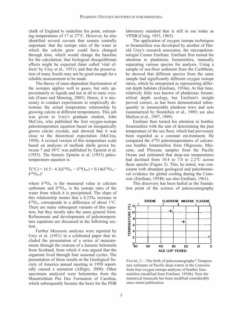
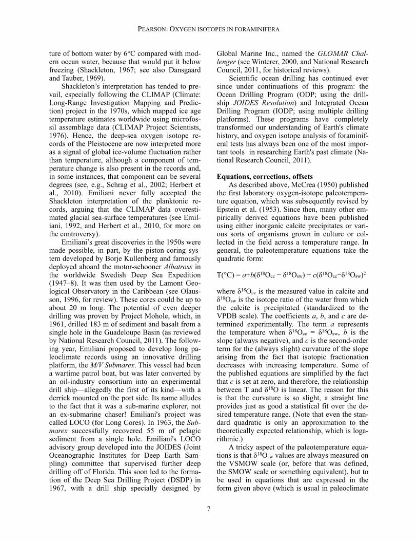
laboratory standard that is still in use today as VPDB (Craig, 1953, 1965). The application of oxygen isotope techniques to foraminifera was developed by another of Har-old Urey's research associates, the micropaleon-tologist Cesare Emiliani. Emiliani first turned his attention to planktonic foraminifera, manually separating various species for analysis. Using a sample of sea-floor sediment from the Caribbean, he showed that different species from the same sample had significantly different oxygen isotope ratios, which he interpreted as representing differ-ent depth habitats (Emiliani, 1954a). At that time, relatively little was known of planktonic forami-niferal depth ecology, but Emiliani's insight proved correct, as has been demonstrated subse-quently in innumerable plankton tows and nets (summarized by Hemleben et al., 1989; see also Mulitza et al., 1997, 1999). Emiliani then turned his attention to benthic foraminifera with the aim of determining the past temperature of the sea floor, which had previously been regarded as a constant environment. He compared the δ18O paleotemperatures of calcare-ous benthic foraminifera from Oligocene, Mio-cene, and Pliocene samples from the Pacific Ocean and estimated that deep-sea temperatures had declined from 10.4 to 7.0 to 2.2°C across these epochs (Figure 2). This, he noted, was con-sistent with abundant geological and paleobotani-cal evidence for global cooling during the Ceno-zoic (Emiliani, 1954b; see also Emiliani, 1961). This discovery has been hailed as the founda-tion point of the science of paleoceanography


AGE (106 YEARS)

T

EMPE

RATU

RE (o

C)

FIGURE 2.—The birth of paleoceanography? Tempera-ture estimates of Pacific deep waters in the Cenozoic from four oxygen isotope analyses of benthic fora-minifera (modified from Emiliani, 1954b). Note the numerical timescale has been modified considerably since initial publication.

5

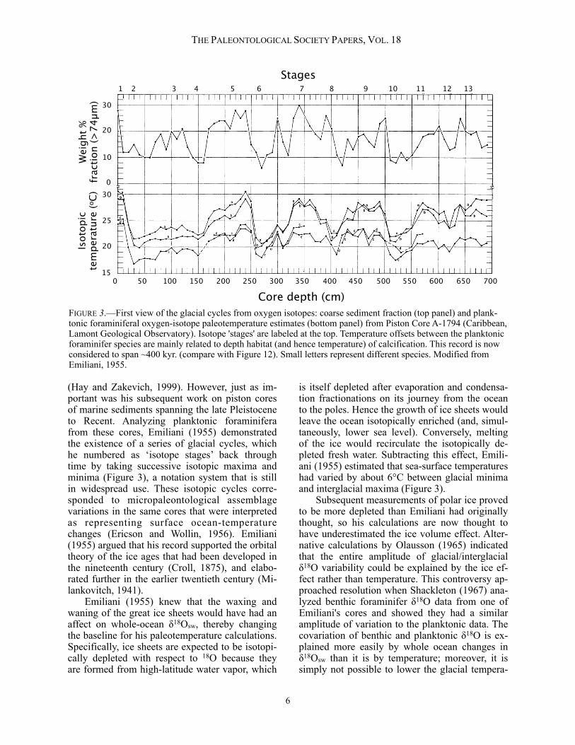
(Hay and Zakevich, 1999). However, just as im-portant was his subsequent work on piston cores of marine sediments spanning the late Pleistocene to Recent. Analyzing planktonic foraminifera from these cores, Emiliani (1955) demonstrated the existence of a series of glacial cycles, which he numbered as ‘isotope stages’ back through time by taking successive isotopic maxima and minima (Figure 3), a notation system that is still in widespread use. These isotopic cycles corre-sponded to micropaleontological assemblage variations in the same cores that were interpreted as representing surface ocean-temperature changes (Ericson and Wollin, 1956). Emiliani (1955) argued that his record supported the orbital theory of the ice ages that had been developed in the nineteenth century (Croll, 1875), and elabo-rated further in the earlier twentieth century (Mi-lankovitch, 1941). Emiliani (1955) knew that the waxing and waning of the great ice sheets would have had an affect on whole-ocean δ18Osw, thereby changing the baseline for his paleotemperature calculations. Specifically, ice sheets are expected to be isotopi-cally depleted with respect to 18O because they are formed from high-latitude water vapor, which

is itself depleted after evaporation and condensa-tion fractionations on its journey from the ocean to the poles. Hence the growth of ice sheets would leave the ocean isotopically enriched (and, simul-taneously, lower sea level). Conversely, melting of the ice would recirculate the isotopically de-pleted fresh water. Subtracting this effect, Emili-ani (1955) estimated that sea-surface temperatures had varied by about 6°C between glacial minima and interglacial maxima (Figure 3). Subsequent measurements of polar ice proved to be more depleted than Emiliani had originally thought, so his calculations are now thought to have underestimated the ice volume effect. Alter-native calculations by Olausson (1965) indicated that the entire amplitude of glacial/interglacial δ18O variability could be explained by the ice ef-fect rather than temperature. This controversy ap-proached resolution when Shackleton (1967) ana-lyzed benthic foraminifer δ18O data from one of Emiliani's cores and showed they had a similar amplitude of variation to the planktonic data. The covariation of benthic and planktonic δ18O is ex-plained more easily by whole ocean changes in δ18Osw than it is by temperature; moreover, it is simply not possible to lower the glacial tempera-


Core depth (cm)0 50 100 150 200 250 300 350 400 450 500 550 600 650 700

Stages1 2 3 4 5 6 7 8 9 10 11 12 13

Isoto

pic

tem

pera

ture

(oC)

Weig

ht %

fract

ion

(>74

m)

15

20

25

300

10

20

30

FIGURE 3.—First view of the glacial cycles from oxygen isotopes: coarse sediment fraction (top panel) and plank-tonic foraminiferal oxygen-isotope paleotemperature estimates (bottom panel) from Piston Core A-1794 (Caribbean, Lamont Geological Observatory). Isotope 'stages' are labeled at the top. Temperature offsets between the planktonic foraminifer species are mainly related to depth habitat (and hence temperature) of calcification. This record is now considered to span ~400 kyr. (compare with Figure 12). Small letters represent different species. Modified from Emiliani, 1955.

6

ture of bottom water by 6°C compared with mod-ern ocean water, because that would put it below freezing (Shackleton, 1967; see also Dansgaard and Tauber, 1969). Shackleton’s interpretation has tended to pre-vail, especially following the CLIMAP (Climate: Long-Range Investigation Mapping and Predic-tion) project in the 1970s, which mapped ice age temperature estimates worldwide using microfos-sil assemblage data (CLIMAP Project Scientists, 1976). Hence, the deep-sea oxygen isotope re-cords of the Pleistocene are now interpreted more as a signal of global ice-volume fluctuation rather than temperature, although a component of tem-perature change is also present in the records and, in some instances, that component can be several degrees (see, e.g., Schrag et al., 2002; Herbert et al., 2010). Emiliani never fully accepted the Shackleton interpretation of the planktonic re-cords, arguing that the CLIMAP data overesti-mated glacial sea-surface temperatures (see Emil-iani, 1992, and Herbert et al., 2010, for more on the controversy). Emiliani’s great discoveries in the 1950s were made possible, in part, by the piston-coring sys-tem developed by Borje Kullenberg and famously deployed aboard the motor-schooner Albatross in the worldwide Swedish Deep Sea Expedition (1947–8). It was then used by the Lamont Geo-logical Observatory in the Caribbean (see Olaus-son, 1996, for review). These cores could be up to about 20 m long. The potential of even deeper drilling was proven by Project Mohole, which, in 1961, drilled 183 m of sediment and basalt from a single hole in the Guadeloupe Basin (as reviewed by National Research Council, 2011). The follow-ing year, Emiliani proposed to develop long pa-leoclimate records using an innovative drilling platform, the M/V Submarex. This vessel had been a wartime patrol boat, but was later converted by an oil-industry consortium into an experimental drill ship—allegedly the first of its kind—with a derrick mounted on the port side. Its name alludes to the fact that it was a sub-marine explorer, not an ex-submarine chaser! Emiliani's project was called LOCO (for Long Cores). In 1963, the Sub-marex successfully recovered 55 m of pelagic sediment from a single hole. Emiliani's LOCO advisory group developed into the JOIDES (Joint Oceanographic Institutes for Deep Earth Sam-pling) committee that supervised further deep drilling off of Florida. This soon led to the forma-tion of the Deep Sea Drilling Project (DSDP) in 1967, with a drill ship specially designed by

Global Marine Inc., named the GLOMAR Chal-lenger (see Winterer, 2000, and National Research Council, 2011, for historical reviews). Scientific ocean drilling has continued ever since under continuations of this program: the Ocean Drilling Program (ODP; using the drill-ship JOIDES Resolution) and Integrated Ocean Drilling Program (IODP; using multiple drilling platforms). These programs have completely transformed our understanding of Earth's climate history, and oxygen isotope analysis of foraminif-eral tests has always been one of the most impor-tant tools in researching Earth's past climate (Na-tional Research Council, 2011).

Equations, corrections, offsets As described above, McCrea (1950) published the first laboratory oxygen-isotope paleotempera-ture equation, which was subsequently revised by Epstein et al. (1953). Since then, many other em-pirically derived equations have been published using either inorganic calcite precipitates or vari-ous sorts of organisms grown in culture or col-lected in the field across a temperature range. In general, the paleotemperature equations take the quadratic form:

T(°C) = a+b(δ18Occ − δ18Osw) + c(δ18Occ−δ18Osw)2

where δ18Occ is the measured value in calcite and δ18Osw is the isotope ratio of the water from which the calcite is precipitated (standardized to the VPDB scale). The coefficients a, b, and c are de-termined experimentally. The term a represents the temperature when δ18Occ = δ18Osw, b is the slope (always negative), and c is the second-order term for the (always slight) curvature of the slope arising from the fact that isotopic fractionation decreases with increasing temperature. Some of the published equations are simplified by the fact that c is set at zero, and therefore, the relationship between T and δ18O is linear. The reason for this is that the curvature is so slight, a straight line provides just as good a statistical fit over the de-sired temperature range. (Note that even the stan-dard quadratic is only an approximation to the theoretically expected relationship, which is loga-rithmic.) A tricky aspect of the paleotemperature equa-tions is that δ18Osw values are always measured on the VSMOW scale (or, before that was defined, the SMOW scale or something equivalent), but to be used in equations that are expressed in the form given above (which is usual in paleoclimate


7

studies) they must be standardized to the VPDB (or PDB) scale. This means a small but significant correction or conversion factor must be applied to the δ18Osw value. This conversion simultaneously corrects for the following: 1) that the absolute scales are offset from each other; and 2) that there is an experimental difference in the fractionation of the oxygen isotopes that occurs when reacting carbonate with phosphoric acid at 25°C (as is done with calcite samples) versus that caused in the equilibrium between water and CO2 at 25.3°C (as is done with water samples) (see Grossman, 2012, for more details). If this was not compli-cated enough, it is important to appreciate that the accepted value for the (V)SMOW to (V)PDB conversion has changed through time. The origi-nal value taken by Epstein et al. (1953) was thought to be -0.20‰. This was subsequently re-vised to -0.22‰ (Friedmann and O'Neil, 1977) and -0.27‰ (Hut, 1987). When using old equa-tions, it is generally necessary to use the value that was assumed in the original study in order to be faithful to the original calibration (see Bemis et al., 1998, for review). However, as Grossman (2012) points out, that rule does not apply to the original Epstein et al. (1953) equation because it was directly standardized with PDB-derived CO2, so in that case, the currently accepted value of -0.27‰ is appropriate. A problem that gradually became apparent from field studies is that the paleotemperature equations were repeatedly found to give tempera-tures that are slightly too high by ~1–2°C com-pared with in-situ temperature measurements (Shackleton et al., 1973; Kahn, 1979; Williams et al., 1981; Deuser and Ross, 1981; Sautter and Thunell, 1991; Mulitza et al., 2003; see discussion in Bemis et al., 1998). Hence, it seems that some significant (albeit fairly minor overall) vital-effect fractionation may occur in some foraminifera (Shackleton et al., 1973). An experimental break-through was made by Spero (1992), Spero and Lea (1993), and Spero et al. (1997), who found that the carbonate ion concentration [CO32-] and pH local to the planktonic foraminifer test was associated with a significant, additional, negative fractionation of the oxygen isotopes. These pa-rameters might be affected by various biological processes local to the foraminifera. The most no-table of these is the presence of a cloud of photo-synthetic symbionts in some species that would be expected to lower the pH and increase the [CO32-] locally (Rink et al., 1998). In an elegant series of experiments, efforts were made to determine dif-

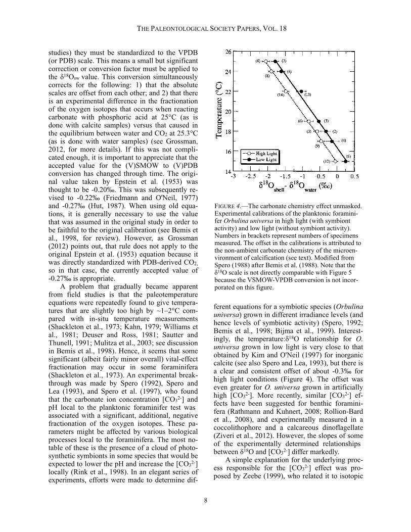
ferent equations for a symbiotic species (Orbulina universa) grown in different irradiance levels (and hence levels of symbiotic activity) (Spero, 1992; Bemis et al., 1998; Bijma et al., 1999). Interest-ingly, the temperature:δ18O relationship for O. universa grown in low light is very close to that obtained by Kim and O'Neil (1997) for inorganic calcite (see also Spero and Lea, 1993), but there is a clear and consistent offset of about -0.3‰ for high light conditions (Figure 4). The offset was even greater for O. universa grown in artificially high [CO32-]. More recently, similar [CO32-] ef-fects have been suggested for benthic foramini-fera (Rathmann and Kuhnert, 2008; Rollion-Bard et al., 2008), and experimentally measured in a coccolithophore and a calcareous dinoflagellate (Ziveri et al., 2012). However, the slopes of some of the experimentally determined relationships between δ18O and [CO32-] differ markedly. A simple explanation for the underlying proc-ess responsible for the [CO32-] effect was pro-posed by Zeebe (1999), who related it to isotopic


FIGURE 4.—The carbonate chemistry effect unmasked. Experimental calibrations of the planktonic foramini-fer Orbulina universa in high light (with symbiont activity) and low light (without symbiont activity). Numbers in brackets represent numbers of specimens measured. The offset in the calibrations is attributed to the non-ambient carbonate chemistry of the microen-vironment of calcification (see text). Modified from Spero (1988) after Bemis et al. (1988). Note that the δ18O scale is not directly comparable with Figure 5 because the VSMOW-VPDB conversion is not incor-porated on this figure.

8

fractionation between the species of dissolved inorganic carbon (H2CO3, HCO3- and CO32-) as a function of pH (Zeebe, 1999). Zeebe (2001) cal-culated a theoretical value of -1.42‰ in δ18O for every 1 unit increase in pH, although experimen-tal determinations of the relationship are still not closely constrained (Spero et al., 1997; Beck et al., 2005). This explanation indicates that the use of the equations such as Kim and O'Neil (1997) would yield temperatures too high by ~1.5°C in symbiotic species. It also suggests that for paleo-applications, a value for pH as well as δ18Osw should be estimated or assumed, especially if large differences in the carbonate system might be expected during the geological past (e.g., Wilson et al., 2002; Bice et al., 2006; Zeebe, 2012), or across some past climatic event (Zeebe et al., 2008; Uchikawa and Zeebe, 2010). Although many shallow-water benthic fora-minifera have photosymbiotic relationships with algae, foraminifera that are commonly used in deep-sea paleoclimate research do not because they live well below the photic zone. One might expect, then, that their paleotemperature curves would lie close to the inorganic relationship. This is indeed the case for some species, but others were found to have consistent offsets (Duplessey et al., 1970; Shackleton and Opdyke, 1973; Shackleton, 1974; Graham et al., 1981; and many subsequent studies). The initial view was that the families Buliminacea (including the common deep-sea genus Uvigerina) and Cassidulinacea give values that are generally close to equilib-rium, whereas the Discorbacea and Rotaliacea (including Cibicidoides) usually give variable negative offsets averaging about -1‰ (Grossman, 1987). Hence, for deep-sea compilations, it be-came standard practice to adjust Cibicidoides val-ues by a fixed number to bring them into line with Uvigerina data (see review by Wefer and Berger, 1991). Subsequently, it has been pointed out (Be-mis et al., 1998; Lynch-Stieglitz et al., 1999; Costa et al., 2006) that if one uses the more recent paleotemperature equation of Kim and O’Neil (1997), Cibicidoides gives values that are closer to equilibrium than does Uvigerina, hence current studies adjust data from other genera to bring them into line with Cibicidoides, and use a paleo-temperature equation calibrated to that genus (e.g., Cramer et al., 2009, 2011). Another problem that must be confronted when using benthic fo-raminiferal δ18O in deep time is that the offsets between common species and genera may have changed over multimillion-year timescales, possi-

bly because of biological evolution (Vincent et al., 1985; Katz et al., 2003). Part of the reason for the offsets between spe-cies of benthic foraminifera may be that some are infaunal and some epifaunal, so they calcify in environments with different pH levels (Bemis et al., 1998; Cramer et al., 2011). Also likely is that while making their test, some foraminifera incor-porate a component of isotopically light metabolic oxygen that originates from their own respired CO2 (Erez, 1978). It has been suggested that spe-cies adapted to low oxygen conditions on the sea floor may have special adaptations enabling oxy-gen exchange with their environment, and so tend to precipitate their tests closer to equilibrium than other species (Grossman, 1987). Several studies have now been published reporting experimental results from deep-sea benthic foraminifera grown in culture (Wilson-Finelli et al., 1998; McCorkle et al., 2008; Barras et al., 2009; Fillipson et al., 2010). The temperature relationships of the cul-tured species are encouragingly close to the pub-lished inorganic paleotemperature relationship. However, there appears to be an additional onto-genetic (growth) effect whereby young/small in-dividuals precipitate their tests with a slight nega-tive offset. This may be because they recycle a higher proportion of oxygen from metabolic CO2 (Barras et al., 2009; Fillipson et al., 2010). In general, the oxygen-isotope technique is very good at identifying relative temperature changes because the slopes of the published rela-tionships are all quite similar, but the possibility of a systematic offset from equilibrium should always be considered in the light of the literature. Clearly, a general rule in any oxygen isotope study based on foraminifera that is designed to determine variations down-core is that a single species should be measured from a restricted size range. This means the sometimes subtle morpho-logical distinctions between species need to be known and appreciated. Considering all this, we come to the question: which paleotemperature equation should one use? There is no right answer to this because it depends on the application. For example, does one prefer an inorganic calibration or one appropriate for the target organism? Which is best, a laboratory cul-ture study or one based on in-situ collections and measurements taken in the ocean? Is a new and more tightly calibrated equation to be preferred to a more widely used historical equation, even if the differences between them are small? To help in this decision, some of the most prominent histori-


9


Reference MaterialCalibra-

tion range (oC)

EquationVSMOW to VPDB

conversion

Epstein et al. (1953) Mollusk shell 7.2–29.5 T(oC) = 16.5 - 4.3 (δ18Occ-δ18Osw) + 0.14 (δ18Occ-δ18Osw) -0.27

O'Neil et al. (1969) reformu-lated by Shackleton (1974)

Synthetic calcite and calcite-water ex-change

0–500 T(oC) = 16.9 - 4.38 (δ18Occ-δ18Osw) + 0.10 (δ18Occ-δ18Osw) -0.20

Horibe and Oba (1972) Cultured mollusks 4.5–23.3T(oC) = 17.04 - 4.34 (δ18Occ-δ18Osw) + 0.16 (δ18Occ-

δ18Osw)-0.20

Erez and Luz (1983)CulturedGlobigerinoides sacculifer (plank-tonic foraminifera)

14–30 T(oC) = 17.0 - 4.52 (δ18Occ-δ18Osw) + 0.03 (δ18Occ-δ18Osw) -0.22

Kim and O'Neil (1997) re-formulated by Bemis et al. (1998)

Synthetic calcite 10–40 T(oC) = 16.1 - 4.64 (δ18Occ-δ18Osw) + 0.09 (δ18Occ-δ18Osw) -0.27

Bemis et al. (1998)Cultured Orbulina universa (high light) (planktonic fora-mininifera)

15–25 T(oC) = 14.9 - 4.80 (δ18Occ-δ18Osw) -0.27

Lynch-Stieglitz et al. (1999) as arranged by Cramer et al. (2011)

In-situ Cibicidoides and Planulina (ben-thic foramininifera)

4–26 T(oC) = 16.1 - 4.76 (δ18Occ-δ18Osw) -0.27

Mielke (2001) in Spero et al. (2003)

Cultured Globoro-talia menardii (planktonic fora-minifera)

? T(oC) = 14.9 - 5.13 (δ18Occ-δ18Osw) -0.27

Spero et al. (unpublished) in Spero et al. (2003)

Cultured Globigeri-noides sacculifer (high light) (plank-tonic foraminifera)

? T(oC) = 12.0 - 5.57 (δ18Occ-δ18Osw) -0.27

Mulitza et al. (2003)In-situ Globigeri-noides sacculifer (high light) (plank-tonic foraminifera)

16–31 T(oC) = 14.91 - 4.35 (δ18Occ-δ18Osw) -0.27

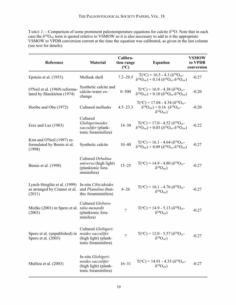
TABLE 1.—Comparison of some prominent paleotemperature equations for calcite δ18O. Note that in each case the δ18Osw term is quoted relative to VSMOW so it is also necessary to add to it the appropriate VSMOW to VPDB conversion current at the time the equation was calibrated, as given in the last column (see text for details).

10

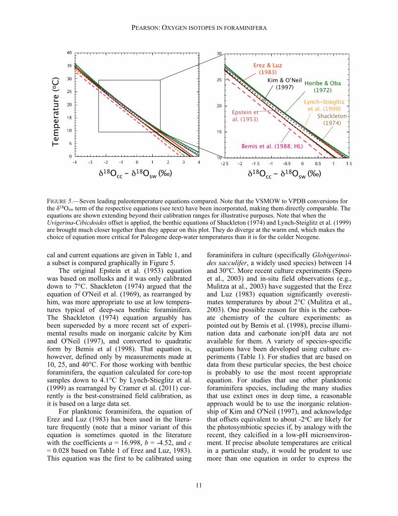
cal and current equations are given in Table 1, and a subset is compared graphically in Figure 5. The original Epstein et al. (1953) equation was based on mollusks and it was only calibrated down to 7°C. Shackleton (1974) argued that the equation of O'Neil et al. (1969), as rearranged by him, was more appropriate to use at low tempera-tures typical of deep-sea benthic foraminifera. The Shackleton (1974) equation arguably has been superseded by a more recent set of experi-mental results made on inorganic calcite by Kim and O'Neil (1997), and converted to quadratic form by Bemis et al (1998). That equation is, however, defined only by measurements made at 10, 25, and 40°C. For those working with benthic foraminifera, the equation calculated for core-top samples down to 4.1°C by Lynch-Stieglitz et al. (1999) as rearranged by Cramer et al. (2011) cur-rently is the best-constrained field calibration, as it is based on a large data set. For planktonic foraminifera, the equation of Erez and Luz (1983) has been used in the litera-ture frequently (note that a minor variant of this equation is sometimes quoted in the literature with the coefficients a = 16.998, b = -4.52, and c = 0.028 based on Table 1 of Erez and Luz, 1983). This equation was the first to be calibrated using

foraminifera in culture (specifically Globigerinoi-des sacculifer, a widely used species) between 14 and 30°C. More recent culture experiments (Spero et al., 2003) and in-situ field observations (e.g., Mulitza at al., 2003) have suggested that the Erez and Luz (1983) equation significantly overesti-mates temperatures by about 2°C (Mulitza et al., 2003). One possible reason for this is the carbon-ate chemistry of the culture experiments: as pointed out by Bemis et al. (1998), precise illumi-nation data and carbonate ion/pH data are not available for them. A variety of species-specific equations have been developed using culture ex-periments (Table 1). For studies that are based on data from these particular species, the best choice is probably to use the most recent appropriate equation. For studies that use other planktonic foraminifera species, including the many studies that use extinct ones in deep time, a reasonable approach would be to use the inorganic relation-ship of Kim and O'Neil (1997), and acknowledge that offsets equivalent to about -2oC are likely for the photosymbiotic species if, by analogy with the recent, they calcified in a low-pH microenviron-ment. If precise absolute temperatures are critical in a particular study, it would be prudent to use more than one equation in order to express the


FIGURE 5.—Seven leading paleotemperature equations compared. Note that the VSMOW to VPDB conversions for the δ18Osw term of the respective equations (see text) have been incorporated, making them directly comparable. The equations are shown extending beyond their calibration ranges for illustrative purposes. Note that when the Uvigerina-Cibicdoides offset is applied, the benthic equations of Shackleton (1974) and Lynch-Steiglitz et al. (1999) are brought much closer together than they appear on this plot. They do diverge at the warm end, which makes the choice of equation more critical for Paleogene deep-water temperatures than it is for the colder Neogene.

Bemis et al. (1988; HL)

Erez & Luz(1983)

Lynch-Stieglitzet al. (1999)Epstein et

al. (1953) Shackleton(1974)

(1997)

18Occ - 18Osw (‰)

Tem

pera

ture

(oC)

18Occ - 18Osw (‰)

Horibe & Oba(1972)

11

uncertainty associated with the choice of equa-tion.

Regional and temporal variations in δ18Osw The most significant complicating factor of using δ18Occ as a paleotemperature indicator is, of course, that it depends on knowing δ18Osw (Urey, 1947). However, this can also be viewed posi-tively because if temperature is known, assumed, or determined (for example, by using another proxy), the method can be used in reverse to in-vestigate regional variations in δ18Osw, or to track the growth and decay of ice sheets through time. The δ18O of seawater can be thought of as reflect-ing two principal factors: 1) interregional variabil-ity that exists at any one time; and 2) the mean value of δ18Osw for the oceans as a whole, which can change over geological time. The δ18O of bottom waters depends on the source area or areas for that water and its history of advection: the transport, mixing, upwelling, and downwelling of ocean currents (Rohling and Cooke, 1999). Consequently, the δ18O of epifau-nal benthic foraminifera can be used (along with several other geochemical tools) to fingerprint deep water masses (Broecker and Peng, 1982). One especially important process that oxygen iso-topes can help identify is sea-ice formation, which expels dense brines with strongly depleted δ18O values. The volume and distribution of such brines influences patterns of deep-water formation and is of potential significance in influencing the global thermohaline circulation of the oceans (Dokken and Jansen, 1999). The influence of brine formation on bottom-water δ18O, as re-flected in benthic foraminiferal data, is especially marked in enclosed basins such as the Weddell Sea in the Southern Hemisphere and the Barents and Nordic seas in the Northern Hemisphere (e.g., Vidal et al., 1998; Mackensen, 2001; Rasmussen and Thomsen, 2009). The principal factor governing the regional δ18O of modern surface seawater is the local evaporation-precipitation (E-P) balance. Because the salinity of seawater also depends on E-P, the two are often correlated, and the variability is sometimes referred to as a salinity effect on δ18Osw. This is clearly only shorthand, however, because the δ18O of precipitation varies system-atically with latitude (which changes the slope of the correlation; Craig, 1965), and additional vari-ability is caused by factors such as river waters flowing into the ocean, iceberg melting, the local climate regime, and advection (see Rohling and

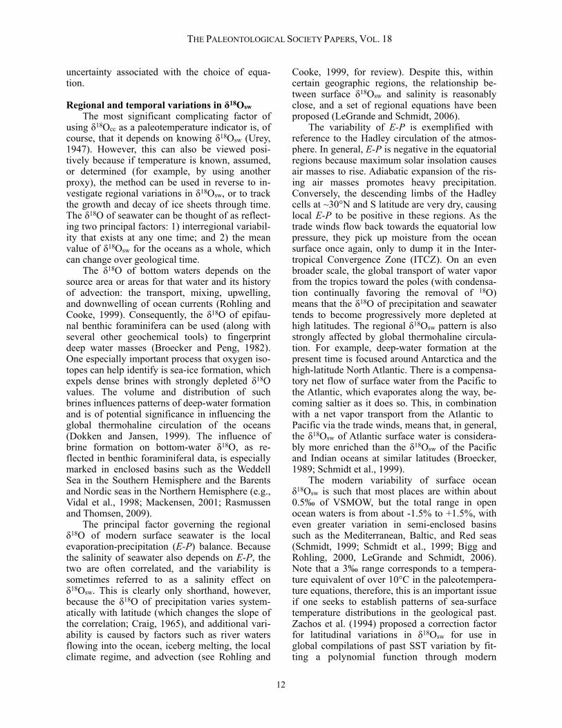
Cooke, 1999, for review). Despite this, within certain geographic regions, the relationship be-tween surface δ18Osw and salinity is reasonably close, and a set of regional equations have been proposed (LeGrande and Schmidt, 2006). The variability of E-P is exemplified with reference to the Hadley circulation of the atmos-phere. In general, E-P is negative in the equatorial regions because maximum solar insolation causes air masses to rise. Adiabatic expansion of the ris-ing air masses promotes heavy precipitation. Conversely, the descending limbs of the Hadley cells at ~30°N and S latitude are very dry, causing local E-P to be positive in these regions. As the trade winds flow back towards the equatorial low pressure, they pick up moisture from the ocean surface once again, only to dump it in the Inter-tropical Convergence Zone (ITCZ). On an even broader scale, the global transport of water vapor from the tropics toward the poles (with condensa-tion continually favoring the removal of 18O) means that the δ18O of precipitation and seawater tends to become progressively more depleted at high latitudes. The regional δ18Osw pattern is also strongly affected by global thermohaline circula-tion. For example, deep-water formation at the present time is focused around Antarctica and the high-latitude North Atlantic. There is a compensa-tory net flow of surface water from the Pacific to the Atlantic, which evaporates along the way, be-coming saltier as it does so. This, in combination with a net vapor transport from the Atlantic to Pacific via the trade winds, means that, in general, the δ18Osw of Atlantic surface water is considera-bly more enriched than the δ18Osw of the Pacific and Indian oceans at similar latitudes (Broecker, 1989; Schmidt et al., 1999). The modern variability of surface ocean δ18Osw is such that most places are within about 0.5‰ of VSMOW, but the total range in open ocean waters is from about -1.5% to +1.5%, with even greater variation in semi-enclosed basins such as the Mediterranean, Baltic, and Red seas (Schmidt, 1999; Schmidt et al., 1999; Bigg and Rohling, 2000, LeGrande and Schmidt, 2006). Note that a 3‰ range corresponds to a tempera-ture equivalent of over 10°C in the paleotempera-ture equations, therefore, this is an important issue if one seeks to establish patterns of sea-surface temperature distributions in the geological past. Zachos et al. (1994) proposed a correction factor for latitudinal variations in δ18Osw for use in global compilations of past SST variation by fit-ting a polynomial function through modern


12

Southern Hemisphere δ18Osw data:

δ18Osw= 0.576 + 0.041x − 0.0017x2 + 0.0000135x3

where x is absolute latitude (N or S) in the range 0–70° (Figure 6). Note that this equation is quite deliberately a blunt tool: it is based only on data from the Southern Hemisphere, but is intended for use in both hemispheres and in deep geological time. It avoids the poles because of the unknown influence of ice (or lack of it). The idea is that it can be used in non-analogue conditions, such as the Paleogene oceans, when different global cir-culation patterns may have operated and a net flow of surface water to the Atlantic cannot be assumed. The Zachos et al. (1994) latitude correction continues to find favor in deep-time paleoclimate studies (e.g., Hollis et al., 2012). It is, however, less appropriate for assessing sites influenced by boundary currents where the latitudinal relation-ship barely applies, and it was never intended for marginal or semi-isolated basins. Moreover, the fundamental relationship between δ18Osw and lati-tude is very likely to have changed through time, especially in the transition from a greenhouse to icehouse climate in the early Oligocene (Bice et al., 2000; Huber et al., 2003). A promising alter-native is to extract surface δ18Osw values for study sites from General Circulation Models. Such models use imposed paleogeographies and green-house gas forcings to simulate past atmospheric and oceanic circulation patterns. In modern isotope-enabled GCMs, the oxygen isotope frac-tionations are also modeled (Schmidt, 1999; Hu-ber et al., 2003; Tindall et al., 2010; Roberts et al., 2011). However, as pointed out by Roberts et al. (2011) and Hollis et al. (in press), these values are strongly dependent on the particular simulation used. The mean value of δ18Osw varies through geo-logical time mainly because of changes in the amount of continental ice, and changes in the rock cycle, principally chemical weathering of rocks and the interaction of seafloor basalts and seawa-ter. The rock-cycle processes are slow, but could become significant at the ~1‰ level over times-cales of 108 years or more (Veizer et al., 1999; Wallmann, 2001; Jaffrés et al., 2007). Much evi-dence exists, for example, that δ18O values of early Paleozoic brachiopods are significantly de-pleted by several parts per mil compared to com-parable Mesozoic and Cenozoic fossils, and a very long-term change in δ18Osw may be partly

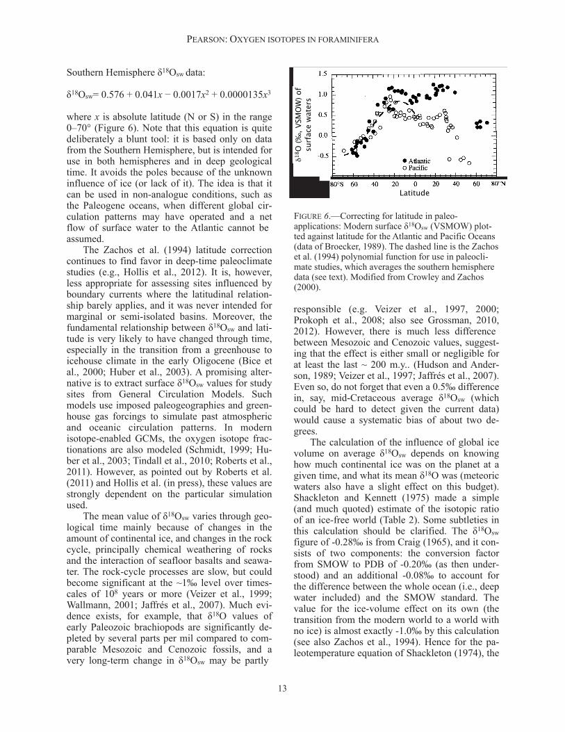
responsible (e.g. Veizer et al., 1997, 2000; Prokoph et al., 2008; also see Grossman, 2010, 2012). However, there is much less difference between Mesozoic and Cenozoic values, suggest-ing that the effect is either small or negligible for at least the last ~ 200 m.y.. (Hudson and Ander-son, 1989; Veizer et al., 1997; Jaffrés et al., 2007). Even so, do not forget that even a 0.5‰ difference in, say, mid-Cretaceous average δ18Osw (which could be hard to detect given the current data) would cause a systematic bias of about two de-grees. The calculation of the influence of global ice volume on average δ18Osw depends on knowing how much continental ice was on the planet at a given time, and what its mean δ18O was (meteoric waters also have a slight effect on this budget). Shackleton and Kennett (1975) made a simple (and much quoted) estimate of the isotopic ratio of an ice-free world (Table 2). Some subtleties in this calculation should be clarified. The δ18Osw figure of -0.28‰ is from Craig (1965), and it con-sists of two components: the conversion factor from SMOW to PDB of -0.20‰ (as then under-stood) and an additional -0.08‰ to account for the difference between the whole ocean (i.e., deep water included) and the SMOW standard. The value for the ice-volume effect on its own (the transition from the modern world to a world with no ice) is almost exactly -1.0‰ by this calculation (see also Zachos et al., 1994). Hence for the pa-leotemperature equation of Shackleton (1974), the


FIGURE 6.—Correcting for latitude in paleo-applications: Modern surface δ18Osw (VSMOW) plot-ted against latitude for the Atlantic and Pacific Oceans (data of Broecker, 1989). The dashed line is the Zachos et al. (1994) polynomial function for use in paleocli-mate studies, which averages the southern hemisphere data (see text). Modified from Crowley and Zachos (2000).

Latitude

18O

(‰, V

SMO

W) o

fsu

rfac

e w

ater

s

13

appropriate value for the δ18Osw term (including the VPDB conversion) is -1.2‰ VSMOW for an ice-free world, whereas for the Erez and Luz (1984) equation, it would be -1.22‰ VSMOW, and for Kim and O'Neil (1997) it would be -1.27‰ VSMOW (see the explanation of appro-priate VSMOW to VPDB conversions, above). The above calculation explains the values for an ice-free world that commonly are encountered in the literature (which are sometimes quoted with the VPDB correction included and sometimes not). However, a more sophisticated approach has now been taken by modeling the growth of present-day ice sheets through their climate his-tory and allowing the δ18O of precipitation (which is now ice buried in the ice sheets) to vary with past climate. Initial calculations indicated that melting of the East Antarctic, West Antarctic, and Greenland ice sheets would respectively contrib-ute -0.91‰, -0.13‰, and -0.07‰ to the ocean, totaling -1.11 ± 0.03‰ for an ice-free ocean (L’Homme et al., 2005). However, it should be noted that Cramer et al. (2011) recalculated the total ice-volume effect using the ice-sheet compo-sitions of L’Homme et al. (2005) and updated val-ues for the mass of the oceans and ice sheets, re-sulting in an estimate of just -0.89‰. At the time of writing, this discrepancy seems unresolved. In either case, for use in a paleotemperature equa-tion, the appropriate VSMOW to VPDB conver-sion term needs to be added (see Table 1).

Depth habitats of planktonic foraminifera As Emiliani (1954a) discovered, planktonic foraminifera are adapted to live across a range of

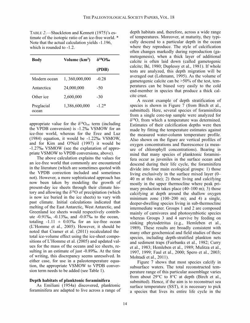
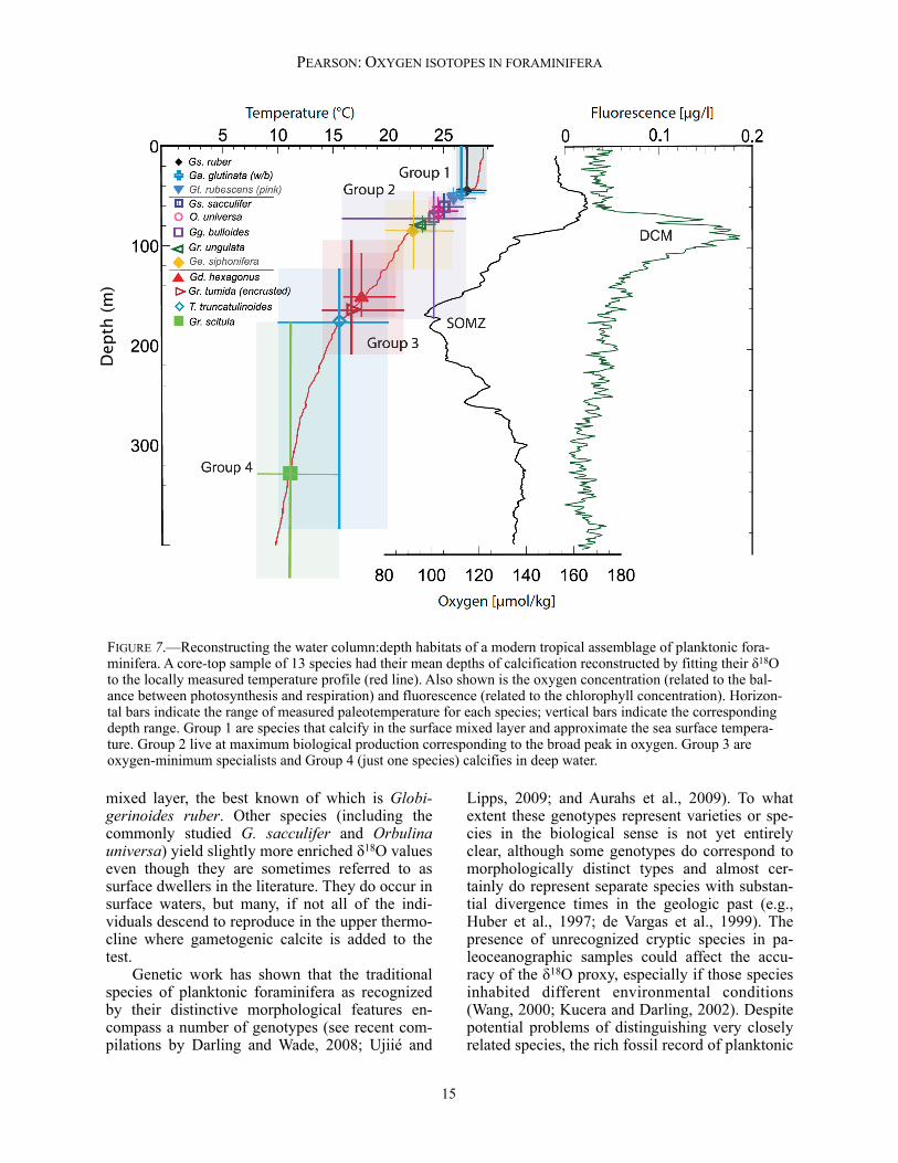
depth habitats and, therefore, across a wide range of temperatures. Moreover, at maturity, they typi-cally descend to a particular depth in the ocean where they reproduce. The style of calcification often changes markedly during reproduction (ga-metogenesis), when a thick layer of additional calcite is often laid down (called gametogenic calcite; Bé, 1980; Duplessy et al., 1981). If whole tests are analyzed, this depth migration will be averaged out (Lohmann, 1995). As the volume of gametogenic calcite can be >50% of the test, tem-peratures can be biased very easily to the cold end-member in species that produce a thick cal-cite crust. A recent example of depth stratification of species is shown in Figure 7 (from Birch et al., submitted). Here, several species of foraminifera from a single core-top sample were analyzed for δ18O, from which a temperature was determined. Estimates of their calcification depths were then made by fitting the temperature estimates against the measured water-column temperature profile. Also shown on the figure are vertical profiles of oxygen concentrations and fluorescence (a meas-ure of chlorophyll concentrations). Bearing in mind that many species of planktonic foramini-fera occur as juveniles in the surface ocean and descend during their life cycle, the foraminifera divide into four main ecological groups: 1) those living exclusively in the surface mixed layer (0–40 m at this site); 2) those living and calcifying mostly in the upper thermocline where peak pri-mary production takes place (40–100 m); 3) those calcifying at depth around the shallow oxygen minimum zone (100–200 m); and 4) a single, deeper-dwelling species living in sub-thermocline intermediate water. Groups 1 and 2 are composed mainly of carnivores and photosymbiotic species whereas Groups 3 and 4 survive by feeding on sinking phytodetritus (e.g., Hemleben et al., 1989). These results are broadly consistent with many other geochemical and field studies of these species, including depth-stratified plankton nets and sediment traps (Fairbanks et al., 1982; Curry et al., 1983; Hemleben et al., 1989; Mulitza et al., 1997, 1999; Faul et al., 2000; Spero et al., 2003; Mohtadi et al., 2011). Figure 7 shows that most species calcify in subsurface waters. The total reconstructed tem-perature range of this particular assemblage varies from about 29°C to 8°C at depth (Birch et al., submitted). Hence, if the aim is to reconstruct sea surface temperature (SST), it is necessary to pick a species that lives its entire life cycle in the


TABLE 2.—Shackleton and Kennett (1975)’s es-timate of the isotopic ratio of an ice-free world. * Note that the actual calculation yields -1.196, which is rounded to -1.2.

Body Volume (km3) δ18O‰

(PDB)

Modern ocean 1, 360,000,000 -0.28

Antarctica 24,000,000 -50

Other ice 2,600,000 -30

Preglacial ocean

1,386,600,000 -1.2*

14

mixed layer, the best known of which is Globi-gerinoides ruber. Other species (including the commonly studied G. sacculifer and Orbulina universa) yield slightly more enriched δ18O values even though they are sometimes referred to as surface dwellers in the literature. They do occur in surface waters, but many, if not all of the indi-viduals descend to reproduce in the upper thermo-cline where gametogenic calcite is added to the test. Genetic work has shown that the traditional species of planktonic foraminifera as recognized by their distinctive morphological features en-compass a number of genotypes (see recent com-pilations by Darling and Wade, 2008; Ujiié and

Lipps, 2009; and Aurahs et al., 2009). To what extent these genotypes represent varieties or spe-cies in the biological sense is not yet entirely clear, although some genotypes do correspond to morphologically distinct types and almost cer-tainly do represent separate species with substan-tial divergence times in the geologic past (e.g., Huber et al., 1997; de Vargas et al., 1999). The presence of unrecognized cryptic species in pa-leoceanographic samples could affect the accu-racy of the δ18O proxy, especially if those species inhabited different environmental conditions (Wang, 2000; Kucera and Darling, 2002). Despite potential problems of distinguishing very closely related species, the rich fossil record of planktonic


FIGURE 7.—Reconstructing the water column:depth habitats of a modern tropical assemblage of planktonic fora-minifera. A core-top sample of 13 species had their mean depths of calcification reconstructed by fitting their δ18O to the locally measured temperature profile (red line). Also shown is the oxygen concentration (related to the bal-ance between photosynthesis and respiration) and fluorescence (related to the chlorophyll concentration). Horizon-tal bars indicate the range of measured paleotemperature for each species; vertical bars indicate the corresponding depth range. Group 1 are species that calcify in the surface mixed layer and approximate the sea surface tempera-ture. Group 2 live at maximum biological production corresponding to the broad peak in oxygen. Group 3 are oxygen-minimum specialists and Group 4 (just one species) calcifies in deep water.

Dept

h (m

)

15

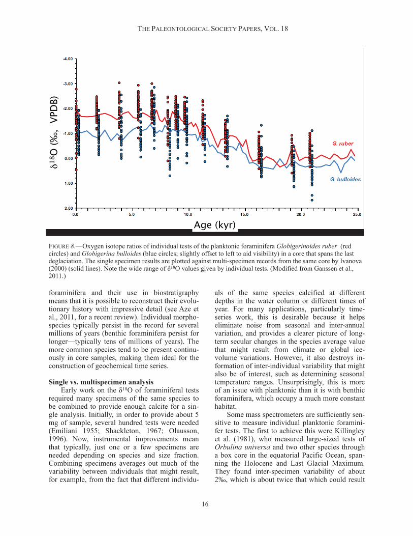
foraminifera and their use in biostratigraphy means that it is possible to reconstruct their evolu-tionary history with impressive detail (see Aze et al., 2011, for a recent review). Individual morpho-species typically persist in the record for several millions of years (benthic foraminifera persist for longer—typically tens of millions of years). The more common species tend to be present continu-ously in core samples, making them ideal for the construction of geochemical time series.

Single vs. multispecimen analysis Early work on the δ18O of foraminiferal tests required many specimens of the same species to be combined to provide enough calcite for a sin-gle analysis. Initially, in order to provide about 5 mg of sample, several hundred tests were needed (Emiliani 1955; Shackleton, 1967; Olausson, 1996). Now, instrumental improvements mean that typically, just one or a few specimens are needed depending on species and size fraction. Combining specimens averages out much of the variability between individuals that might result, for example, from the fact that different individu-

als of the same species calcified at different depths in the water column or different times of year. For many applications, particularly time-series work, this is desirable because it helps eliminate noise from seasonal and inter-annual variation, and provides a clearer picture of long-term secular changes in the species average value that might result from climate or global ice-volume variations. However, it also destroys in-formation of inter-individual variability that might also be of interest, such as determining seasonal temperature ranges. Unsurprisingly, this is more of an issue with planktonic than it is with benthic foraminifera, which occupy a much more constant habitat. Some mass spectrometers are sufficiently sen-sitive to measure individual planktonic foramini-fer tests. The first to achieve this were Killingley et al. (1981), who measured large-sized tests of Orbulina universa and two other species through a box core in the equatorial Pacific Ocean, span-ning the Holocene and Last Glacial Maximum. They found inter-specimen variability of about 2‰, which is about twice that which could result


FIGURE 8.—Oxygen isotope ratios of individual tests of the planktonic foraminifera Globigerinoides ruber (red circles) and Globigerina bulloides (blue circles; slightly offset to left to aid visibility) in a core that spans the last deglaciation. The single specimen results are plotted against multi-specimen records from the same core by Ivanova (2000) (solid lines). Note the wide range of δ18O values given by individual tests. (Modified from Ganssen et al., 2011.)

Age (kyr)

18O

(‰

, V

PD

B)

16

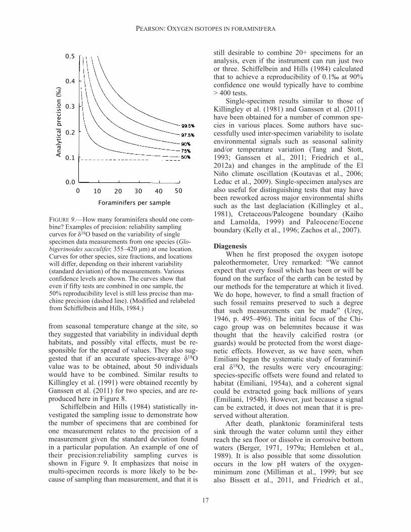
from seasonal temperature change at the site, so they suggested that variability in individual depth habitats, and possibly vital effects, must be re-sponsible for the spread of values. They also sug-gested that if an accurate species-average δ18O value was to be obtained, about 50 individuals would have to be combined. Similar results to Killingley et al. (1991) were obtained recently by Ganssen et al. (2011) for two species, and are re-produced here in Figure 8. Schiffelbein and Hills (1984) statistically in-vestigated the sampling issue to demonstrate how the number of specimens that are combined for one measurement relates to the precision of a measurement given the standard deviation found in a particular population. An example of one of their precision:reliability sampling curves is shown in Figure 9. It emphasizes that noise in multi-specimen records is more likely to be be-cause of sampling than measurement, and that it is

still desirable to combine 20+ specimens for an analysis, even if the instrument can run just two or three. Schiffelbein and Hills (1984) calculated that to achieve a reproducibility of 0.1‰ at 90% confidence one would typically have to combine > 400 tests. Single-specimen results similar to those of Killingley et al. (1981) and Ganssen et al. (2011) have been obtained for a number of common spe-cies in various places. Some authors have suc-cessfully used inter-specimen variability to isolate environmental signals such as seasonal salinity and/or temperature variation (Tang and Stott, 1993; Ganssen et al., 2011; Friedrich et al., 2012a) and changes in the amplitude of the El Niño climate oscillation (Koutavas et al., 2006; Leduc et al., 2009). Single-specimen analyses are also useful for distinguishing tests that may have been reworked across major environmental shifts such as the last deglaciation (Killingley et al., 1981), Cretaceous/Paleogene boundary (Kaiho and Lamolda, 1999) and Paleocene/Eocene boundary (Kelly et al., 1996; Zachos et al., 2007).

Diagenesis When he first proposed the oxygen isotope paleothermometer, Urey remarked: “We cannot expect that every fossil which has been or will be found on the surface of the earth can be tested by our methods for the temperature at which it lived. We do hope, however, to find a small fraction of such fossil remains preserved to such a degree that such measurements can be made” (Urey, 1946, p. 495–496). The initial focus of the Chi-cago group was on belemnites because it was thought that the heavily calcified rostra (or guards) would be protected from the worst diage-netic effects. However, as we have seen, when Emiliani began the systematic study of foraminif-eral δ18O, the results were very encouraging: species-specific offsets were found and related to habitat (Emiliani, 1954a), and a coherent signal could be extracted going back millions of years (Emiliani, 1954b). However, just because a signal can be extracted, it does not mean that it is pre-served without alteration. After death, planktonic foraminiferal tests sink through the water column until they either reach the sea floor or dissolve in corrosive bottom waters (Berger, 1971, 1979a; Hemleben et al., 1989). It is also possible that some dissolution occurs in the low pH waters of the oxygen-minimum zone (Milliman et al., 1999; but see also Bissett et al., 2011, and Friedrich et al.,


0 10 20 30 40 50Foraminifers per sample

Analy

tical

prec

ision

(‰)

0.0

0.1

0.2

0.3

0.4

0.5

FIGURE 9.—How many foraminifera should one com-bine? Examples of precision: reliability sampling curves for δ18O based on the variability of single specimen data measurements from one species (Glo-bigerinoides sacculifer, 355–420 µm) at one location. Curves for other species, size fractions, and locations will differ, depending on their inherent variability (standard deviation) of the measurements. Various confidence levels are shown. The curves show that even if fifty tests are combined in one sample, the 50% reproducibility level is still less precise than ma-chine precision (dashed line). (Modified and relabeled from Schiffelbein and Hills, 1984.)

17

2012a, who suggest water-column effects gener-ally are minimal). Further dissolution in the sedi-ment of both benthic and planktonic foraminiferal tests can be promoted by low pH associated with the aerobic mineralization of organic matter (Jahnke et al., 1997), or, for oxygen-deficient sediments, exposure to oxygen during storage of the cores themselves (Self-Trail and Seefelt, 2004). The external gametogenic calcite often is more resistant to dissolution, so tests can become hollowed out with the internal chamber wall dis-solved away (Bé et al., 1975). If different phases of the foraminiferal calcite were produced at dif-ferent times in the life cycle, such differential dis-solution potentially could alter the isotopic ratios. This effect can be especially important if an iso-topic record is produced from a site that shows varying dissolution intensities through time. Lohmann (1995) highlighted the importance of

assessing the mass balance between chamber cal-cite and gametogenic crust when considering both the original habitat and the potential effects of dissolution. Precipitation of calcite cements from pore waters is a frequently encountered problem. It can occur on the outside of a test, overgrowing sur-face features, or on the inside, commonly filling the test completely. If this happens during shallow burial, the cements are likely to have a more en-riched δ18O than the original plankton tests, but if cements are formed at high temperatures after substantial burial, the opposite will be the case (Schrag, 1999). Diagenetic cements formed from percolating meteoric waters (which are often en-countered in geological sections emplaced on land) also will tend to have depleted δ18O, often by several parts per mil (e.g., Corfield et al., 1990). Clearly, foraminifer tests with substantial


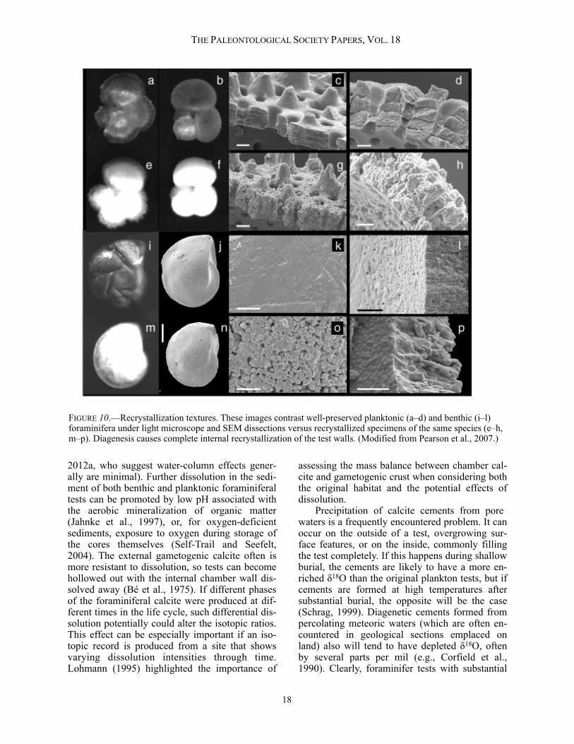
FIGURE 10.—Recrystallization textures. These images contrast well-preserved planktonic (a–d) and benthic (i–l) foraminifera under light microscope and SEM dissections versus recrystallized specimens of the same species (e–h, m–p). Diagenesis causes complete internal recrystallization of the test walls. (Modified from Pearson et al., 2007.)

18

diagenetic overgrowth and infilling are not suit-able for extracting accurate paleoenvironmental information. Fortunately, such effects are usually plainly visible under the light microscopic and/or scanning electron microscope (SEM) (Pearson and Burgess, 2009). Micron-scale recrystallization of tests, which occurs commonly during the shallow burial of deep-sea carbonate oozes, is more of a problem. The biogenic texture of most foraminifer tests is microgranular, with individual granules or plaques in the ~0.1 µm size range and having ir-regular shapes. However, this texture is com-monly replaced entirely by larger, more-equant neomorphic calcite crystals in the ~1 µm range (Pearson et al., 2001). This wholesale recrystalli-zation can cause very substantial alteration of the oxygen-isotope ratios (Pearson et al., 2001, 2007; Williams et al., 2004; Sexton et al., 2006). Per-haps because a component of the original isotopic signature remains after recrystallization, this problem was not fully appreciated for many years,

so claims in the literature that foraminifera are well preserved cannot always be relied upon. Pearson and Burgess (2009) proposed the follow-ing criteria for recognizing exceptionally pre-served tests: (1) tests should be reflective and translucent under reflective light, especially the smaller, thin-walled species; (2) when placed in water or oil, ultrafine features smaller than a mi-cron should survive (e.g. spines, if originally pre-sent); (3) originally smooth parts of the test sur-face and interior should still be smooth on a sub-micron scale; and (4) the original submicron granular texture should be visible in cross-section when the test is broken. These features are illustrated in Figure 10. It was originally hoped that benthic foraminifera might be less prone to recrystallization than planktonic forms because of their denser calcite microstructures (Pearson et al., 2001), but it seems that this is not the case (Sexton et al., 2006; Pearson et al., 2007; Figure 10). Unfortunately, recrystallization is nearly ubiquitous in deep-sea


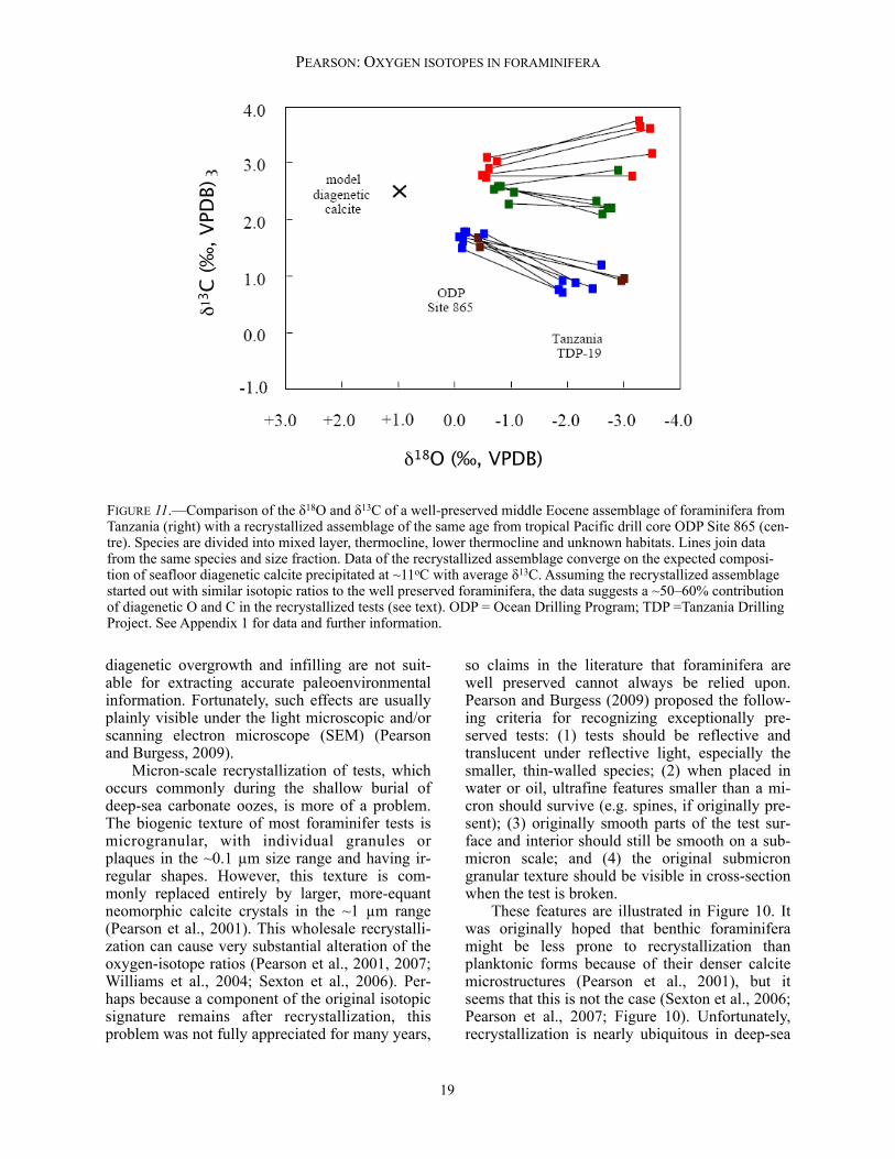
FIGURE 11.—Comparison of the δ18O and δ13C of a well-preserved middle Eocene assemblage of foraminifera from Tanzania (right) with a recrystallized assemblage of the same age from tropical Pacific drill core ODP Site 865 (cen-tre). Species are divided into mixed layer, thermocline, lower thermocline and unknown habitats. Lines join data from the same species and size fraction. Data of the recrystallized assemblage converge on the expected composi-tion of seafloor diagenetic calcite precipitated at ~11oC with average δ13C. Assuming the recrystallized assemblage started out with similar isotopic ratios to the well preserved foraminifera, the data suggests a ~50–60% contribution of diagenetic O and C in the recrystallized tests (see text). ODP = Ocean Drilling Program; TDP =Tanzania Drilling Project. See Appendix 1 for data and further information.

3C

(‰

, V

PD

B)

18O (‰, VPDB)

19

carbonate oozes and chalks of substantial geo-logic age (millions of years). On the other hand, well-preserved foraminifera generally are found in hemipelagic clays, where the low permeability presumably inhibits the recrystallization process (e.g., Norris and Wilson, 1998; Pearson et al., 2001; Wilson et al., 2002; Sexton et al., 2006; Pearson and Wade, 2009). The effect of diagenetic recrystallization on the oxygen and carbon isotope ratios of plank-tonic foraminiferal assemblages is shown in Fig-ure 11, which compares two assemblages of mid-dle Eocene foraminifera, one well-preserved and the other recrystallized. This type of comparison, although never exact, suggests that recrystallized assemblages are partially homogenized in their isotope ratios, reducing interspecies differentials, and converging on the expected value for diage-netic calcite. Because the δ13C of diagenetic cal-cite is similar to an average value of the foramini-fera, the absolute values do not change much. However, the oxygen isotope ratio of inorganic calcite on the sea floor is very different from the original planktonic values because of the colder temperatures, so the shift in δ18O is much more substantial. This point was made by Pearson et al. (2001, their fig. 4) in a similar diagram; data for Figure 11 and further details are given in the Ap-p e n d i x a n d o n l i n e s p r e a d s h e e t a t <http://paleosoc.org/shortcourse2012.html>. Note that although benthic foraminifera may be recrys-tallized, the effect on their δ18O values is probably relatively small because recrystallization usually occurs at or near the sediment/water interface at nearly the same temperature as the time of fora-minifer shell growth. The impact of the diagenesis problem on the determination of tropical surface temperatures is discussed further below. Kozdon et al. (2011) used an ion microprobe to analyze internal parts of the tests of recrystal-lized foraminifera and compared their values with whole-test measurements. Their results indicate that, although recrystallized, the internal parts of the test have exchanged less isotopically with their environment than the more outer parts of the test. This suggests that internal microprobe measurements may provide a better estimate of the original sea-surface temperature than the whole test. However, some degree of isotopic ex-change cannot be ruled out even for the interior parts of recrystallized tests.

PART 2: APPLICATIONS

In this section, some of the main applications of oxygen isotope analyses of foraminifera are re-viewed under three headings: 1) climate cycles and cyclostratigraphy, 2) deep-time benthic fo-raminiferal compilations, and 3) planktonic fo-raminiferal habitats and sea-surface temperatures. Happily, these three subject areas correspond to Emiliani's troika of papers that helped define the discipline of paleoceanography in its earliest days (Emiliani, 1954b, 1955, and 1954a, respectively).

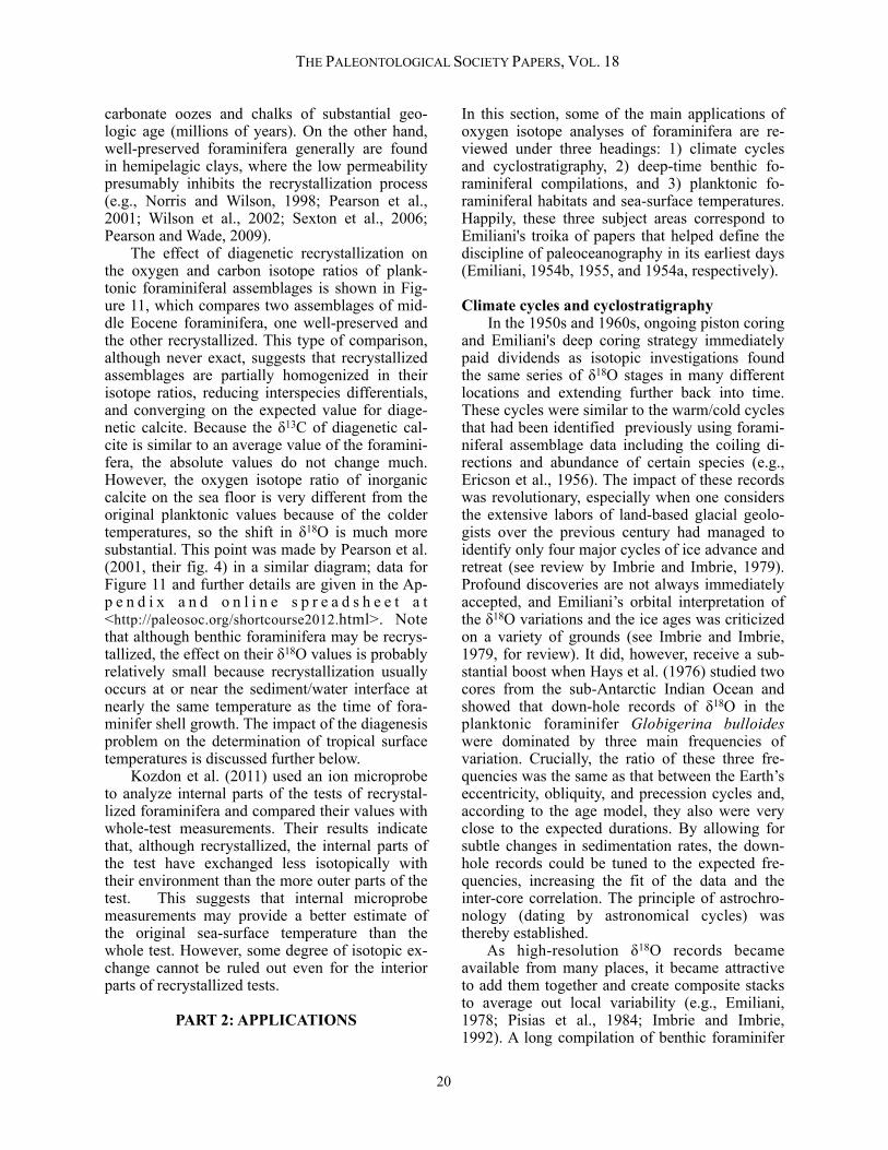
Climate cycles and cyclostratigraphy In the 1950s and 1960s, ongoing piston coring and Emiliani's deep coring strategy immediately paid dividends as isotopic investigations found the same series of δ18O stages in many different locations and extending further back into time. These cycles were similar to the warm/cold cycles that had been identified previously using forami-niferal assemblage data including the coiling di-rections and abundance of certain species (e.g., Ericson et al., 1956). The impact of these records was revolutionary, especially when one considers the extensive labors of land-based glacial geolo-gists over the previous century had managed to identify only four major cycles of ice advance and retreat (see review by Imbrie and Imbrie, 1979). Profound discoveries are not always immediately accepted, and Emiliani’s orbital interpretation of the δ18O variations and the ice ages was criticized on a variety of grounds (see Imbrie and Imbrie, 1979, for review). It did, however, receive a sub-stantial boost when Hays et al. (1976) studied two cores from the sub-Antarctic Indian Ocean and showed that down-hole records of δ18O in the planktonic foraminifer Globigerina bulloides were dominated by three main frequencies of variation. Crucially, the ratio of these three fre-quencies was the same as that between the Earth’s eccentricity, obliquity, and precession cycles and, according to the age model, they also were very close to the expected durations. By allowing for subtle changes in sedimentation rates, the down-hole records could be tuned to the expected fre-quencies, increasing the fit of the data and the inter-core correlation. The principle of astrochro-nology (dating by astronomical cycles) was thereby established. As high-resolution δ18O records became available from many places, it became attractive to add them together and create composite stacks to average out local variability (e.g., Emiliani, 1978; Pisias et al., 1984; Imbrie and Imbrie, 1992). A long compilation of benthic foraminifer


20

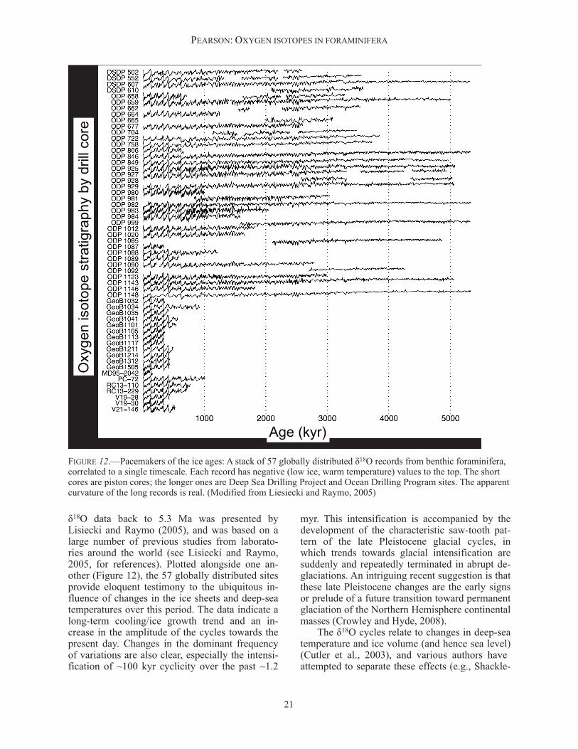
δ18O data back to 5.3 Ma was presented by Lisiecki and Raymo (2005), and was based on a large number of previous studies from laborato-ries around the world (see Lisiecki and Raymo, 2005, for references). Plotted alongside one an-other (Figure 12), the 57 globally distributed sites provide eloquent testimony to the ubiquitous in-fluence of changes in the ice sheets and deep-sea temperatures over this period. The data indicate a long-term cooling/ice growth trend and an in-crease in the amplitude of the cycles towards the present day. Changes in the dominant frequency of variations are also clear, especially the intensi-fication of ~100 kyr cyclicity over the past ~1.2

myr. This intensification is accompanied by the development of the characteristic saw-tooth pat-tern of the late Pleistocene glacial cycles, in which trends towards glacial intensification are suddenly and repeatedly terminated in abrupt de-glaciations. An intriguing recent suggestion is that these late Pleistocene changes are the early signs or prelude of a future transition toward permanent glaciation of the Northern Hemisphere continental masses (Crowley and Hyde, 2008). The δ18O cycles relate to changes in deep-sea temperature and ice volume (and hence sea level) (Cutler et al., 2003), and various authors have attempted to separate these effects (e.g., Shackle-


FIGURE 12.—Pacemakers of the ice ages: A stack of 57 globally distributed δ18O records from benthic foraminifera, correlated to a single timescale. Each record has negative (low ice, warm temperature) values to the top. The short cores are piston cores; the longer ones are Deep Sea Drilling Project and Ocean Drilling Program sites. The apparent curvature of the long records is real. (Modified from Liesiecki and Raymo, 2005)

!"#$%&'()

*+'"#,$-./0/1#$.0(20-"(213'$4'$5(-66$7/(#

21

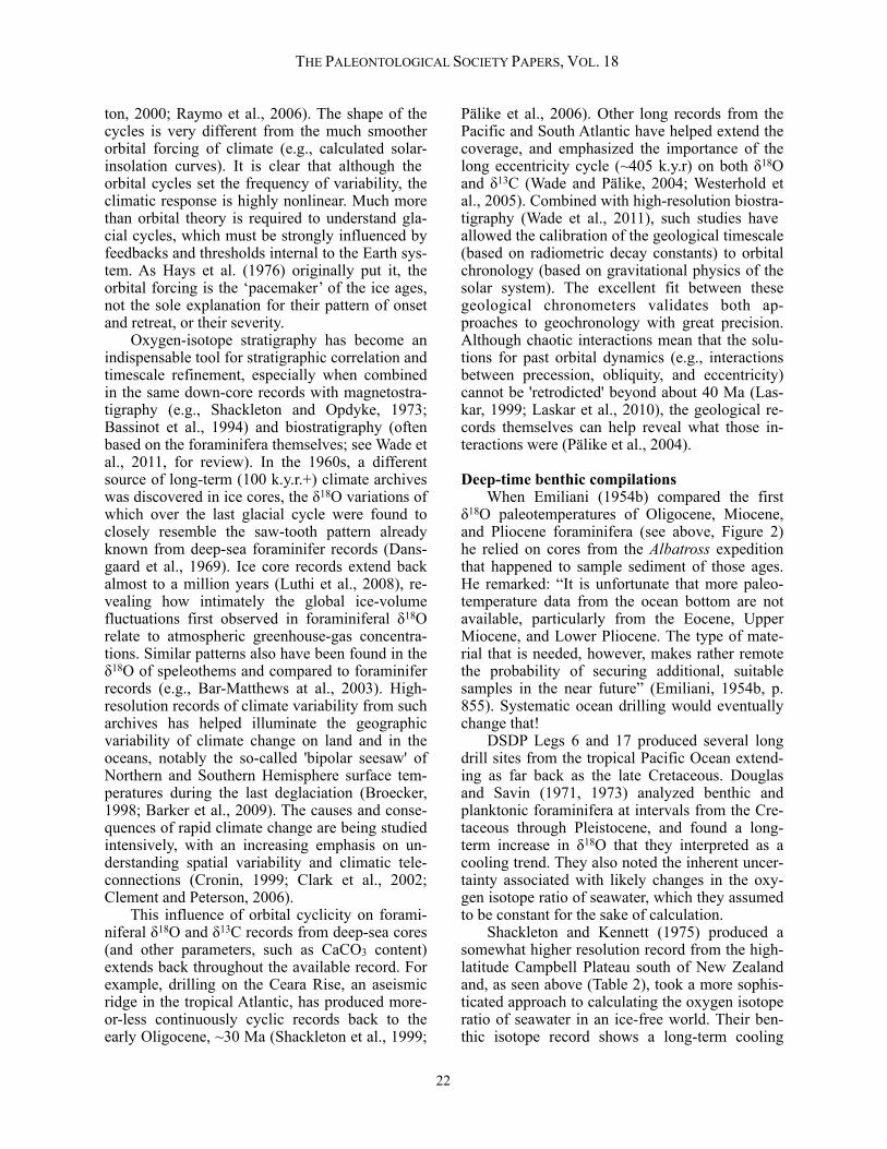
ton, 2000; Raymo et al., 2006). The shape of the cycles is very different from the much smoother orbital forcing of climate (e.g., calculated solar-insolation curves). It is clear that although the orbital cycles set the frequency of variability, the climatic response is highly nonlinear. Much more than orbital theory is required to understand gla-cial cycles, which must be strongly influenced by feedbacks and thresholds internal to the Earth sys-tem. As Hays et al. (1976) originally put it, the orbital forcing is the ‘pacemaker’ of the ice ages, not the sole explanation for their pattern of onset and retreat, or their severity. Oxygen-isotope stratigraphy has become an indispensable tool for stratigraphic correlation and timescale refinement, especially when combined in the same down-core records with magnetostra-tigraphy (e.g., Shackleton and Opdyke, 1973; Bassinot et al., 1994) and biostratigraphy (often based on the foraminifera themselves; see Wade et al., 2011, for review). In the 1960s, a different source of long-term (100 k.y.r.+) climate archives was discovered in ice cores, the δ18O variations of which over the last glacial cycle were found to closely resemble the saw-tooth pattern already known from deep-sea foraminifer records (Dans-gaard et al., 1969). Ice core records extend back almost to a million years (Luthi et al., 2008), re-vealing how intimately the global ice-volume fluctuations first observed in foraminiferal δ18O relate to atmospheric greenhouse-gas concentra-tions. Similar patterns also have been found in the δ18O of speleothems and compared to foraminifer records (e.g., Bar-Matthews at al., 2003). High-resolution records of climate variability from such archives has helped illuminate the geographic variability of climate change on land and in the oceans, notably the so-called 'bipolar seesaw' of Northern and Southern Hemisphere surface tem-peratures during the last deglaciation (Broecker, 1998; Barker et al., 2009). The causes and conse-quences of rapid climate change are being studied intensively, with an increasing emphasis on un-derstanding spatial variability and climatic tele-connections (Cronin, 1999; Clark et al., 2002; Clement and Peterson, 2006). This influence of orbital cyclicity on forami-niferal δ18O and δ13C records from deep-sea cores (and other parameters, such as CaCO3 content) extends back throughout the available record. For example, drilling on the Ceara Rise, an aseismic ridge in the tropical Atlantic, has produced more-or-less continuously cyclic records back to the early Oligocene, ~30 Ma (Shackleton et al., 1999;

Pälike et al., 2006). Other long records from the Pacific and South Atlantic have helped extend the coverage, and emphasized the importance of the long eccentricity cycle (~405 k.y.r) on both δ18O and δ13C (Wade and Pälike, 2004; Westerhold et al., 2005). Combined with high-resolution biostra-tigraphy (Wade et al., 2011), such studies have allowed the calibration of the geological timescale (based on radiometric decay constants) to orbital chronology (based on gravitational physics of the solar system). The excellent fit between these geological chronometers validates both ap-proaches to geochronology with great precision. Although chaotic interactions mean that the solu-tions for past orbital dynamics (e.g., interactions between precession, obliquity, and eccentricity) cannot be 'retrodicted' beyond about 40 Ma (Las-kar, 1999; Laskar et al., 2010), the geological re-cords themselves can help reveal what those in-teractions were (Pälike et al., 2004).

Deep-time benthic compilations When Emiliani (1954b) compared the first δ18O paleotemperatures of Oligocene, Miocene, and Pliocene foraminifera (see above, Figure 2) he relied on cores from the Albatross expedition that happened to sample sediment of those ages. He remarked: “It is unfortunate that more paleo-temperature data from the ocean bottom are not available, particularly from the Eocene, Upper Miocene, and Lower Pliocene. The type of mate-rial that is needed, however, makes rather remote the probability of securing additional, suitable samples in the near future” (Emiliani, 1954b, p. 855). Systematic ocean drilling would eventually change that! DSDP Legs 6 and 17 produced several long drill sites from the tropical Pacific Ocean extend-ing as far back as the late Cretaceous. Douglas and Savin (1971, 1973) analyzed benthic and planktonic foraminifera at intervals from the Cre-taceous through Pleistocene, and found a long-term increase in δ18O that they interpreted as a cooling trend. They also noted the inherent uncer-tainty associated with likely changes in the oxy-gen isotope ratio of seawater, which they assumed to be constant for the sake of calculation. Shackleton and Kennett (1975) produced a somewhat higher resolution record from the high-latitude Campbell Plateau south of New Zealand and, as seen above (Table 2), took a more sophis-ticated approach to calculating the oxygen isotope ratio of seawater in an ice-free world. Their ben-thic isotope record shows a long-term cooling


22

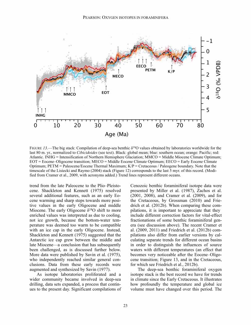
trend from the late Paleocene to the Plio–Pleisto-cene. Shackleton and Kennett (1975) resolved several additional features, such as an early Eo-cene warming and sharp steps towards more posi-tive values in the early Oligocene and middle Miocene. The early Oligocene δ18O shift to more enriched values was interpreted as due to cooling, not ice growth, because the bottom-water tem-perature was deemed too warm to be compatible with an ice cap in the early Oligocene. Instead, Shackleton and Kennett (1975) suggested that the Antarctic ice cap grew between the middle and late Miocene—a conclusion that has subsequently been challenged, as is discussed further below. More data were published by Savin et al. (1975), who independently reached similar general con-clusions. Data from these early records were augmented and synthesized by Savin (1977). As isotope laboratories proliferated and a wider community became involved in deep-sea drilling, data sets expanded, a process that contin-ues to the present day. Significant compilations of

Cenozoic benthic foraminiferal isotope data were presented by Miller et al. (1987), Zachos et al. (2001, 2008), and Cramer et al. (2009), and for the Cretaceous, by Grossman (2010) and Frie-drich et al. (2012b). When comparing these com-pilations, it is important to appreciate that they include different correction factors for vital-effect fractionations of some benthic foraminiferal gen-era (see discussion above). The recent Cramer et al. (2009, 2011) and Friedrich et al. (2012b) com-pilations also differ from earlier versions by cal-culating separate trends for different ocean basins in order to distinguish the influences of source waters with different temperatures (an effect that becomes very noticeable after the Eocene–Oligo-cene transition; Figure 13, and in the Cretaceous, for which see Friedrich et al., 2012b). The deep-sea benthic foraminiferal oxygen isotope stack is the best record we have for trends in climate since the Early Cretaceous. It illustrates how profoundly the temperature and global ice volume must have changed over this period. The


FIGURE 13.—The big stack: Compilation of deep-sea benthic δ18O values obtained by laboratories worldwide for the last 80 m. yr., normalized to Cibicidoides (see text). Black: global mean; blue: southern ocean; orange: Pacific; red: Atlantic. INHG = Intensification of Northern Hemisphere Glaciation; MMCO = Middle Miocene Climate Optimum; EOT = Eocene–Oligocene transition; MECO = Middle Eocene Climate Optimum; EECO = Early Eocene Climate Optimum; PETM = Paleocene/Eocene Thermal Maximum; K/P = Cretaceous / Paleogene boundary. Note that the timescale of the Lisiecki and Raymo (2004) stack (Figure 12) corresponds to the last 5 myr. of this record. (Modi-fied from Cramer et al., 2009, with acronyms added.) Trend lines represent different oceans.

EECOPETM

EOTMMCO

MECOK/P

INHG

0 10 20 30 40 50 60 70 80

5

4

3

2

1

0

-1

Age (Ma)

18O

(‰

VPD

B)

23

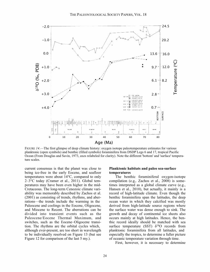
current consensus is that the planet was close to being ice-free in the early Eocene, and seafloor temperatures were about 14°C, compared to only 2–3°C today (Cramer et al., 2011). Global tem-peratures may have been even higher in the mid-Cretaceous. The long-term Cenozoic climate vari-ability was memorably described by Zachos et al. (2001) as consisting of trends, rhythms, and aber-rations—the trends include the warming in the Paleocene and coolings in the Eocene, Oligocene, and Miocene to Recent. The aberrations can be divided into transient events such as the Paleocene/Eocene Thermal Maximum, and switches, such as the Eocene–Oligocene transi-tion. The rhythms are the orbital cycles which, although ever-present, are too short in wavelength to be individually resolved on Figure 13 (but see Figure 12 for comparison of the last 5 my.).

Planktonic habitats and paleo sea-surface temperatures The benthic foraminiferal oxygen-isotope compilation (e.g,. Zachos et al., 2008) is some-times interpreted as a global climate curve (e.g., Hansen et al., 2010), but actually, it mainly is a record of high-latitude climate. Even though the benthic foraminifera span the latitudes, the deep ocean water in which they calcified was mostly derived from high-latitude source regions where the surface water was dense enough to sink. The growth and decay of continental ice sheets also occurs mainly at high latitudes. Hence, the ben-thic record ideally should be matched with sea surface temperature (SST) δ18O records from planktonic foraminifera from all latitudes, and especially the tropics, to determine a fuller picture of oceanic temperature variation through time. First, however, it is necessary to determine


18O

(‰

, PD

B)

+4.0

+3.0

+1.0

0.0

-1.0

-2.0

+2.0

0.7

2.8

6.1

9.7

13.6

8.2

12.0

16.0

20.2

24.5

BO

TTO

M

SU

RFA

CE

Tem

peratu

re (

oC

)

10 30 4020 50 60 70

Age (Ma)

800

FIGURE 14.—The first glimpse of deep climate history: oxygen isotope paleotemperature estimates for various planktonic (open symbols) and benthic (filled symbols) foraminifera from DSDP Legs 6 and 17, tropical Pacific Ocean (From Douglas and Savin, 1973, axes relabeled for clarity). Note the different 'bottom' and 'surface' tempera-ture scales.

24

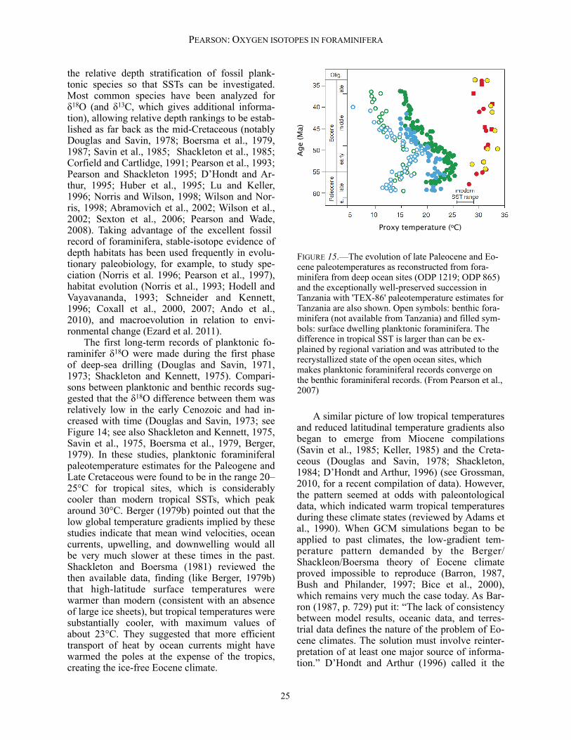
the relative depth stratification of fossil plank-tonic species so that SSTs can be investigated. Most common species have been analyzed for δ18O (and δ13C, which gives additional informa-tion), allowing relative depth rankings to be estab-lished as far back as the mid-Cretaceous (notably Douglas and Savin, 1978; Boersma et al., 1979, 1987; Savin et al., 1985; Shackleton et al., 1985; Corfield and Cartlidge, 1991; Pearson et al., 1993; Pearson and Shackleton 1995; D’Hondt and Ar-thur, 1995; Huber et al., 1995; Lu and Keller, 1996; Norris and Wilson, 1998; Wilson and Nor-ris, 1998; Abramovich et al., 2002; Wilson et al., 2002; Sexton et al., 2006; Pearson and Wade, 2008). Taking advantage of the excellent fossil record of foraminifera, stable-isotope evidence of depth habitats has been used frequently in evolu-tionary paleobiology, for example, to study spe-ciation (Norris et al. 1996; Pearson et al., 1997), habitat evolution (Norris et al., 1993; Hodell and Vayavananda, 1993; Schneider and Kennett, 1996; Coxall et al., 2000, 2007; Ando et al., 2010), and macroevolution in relation to envi-ronmental change (Ezard et al. 2011). The first long-term records of planktonic fo-raminifer δ18O were made during the first phase of deep-sea drilling (Douglas and Savin, 1971, 1973; Shackleton and Kennett, 1975). Compari-sons between planktonic and benthic records sug-gested that the δ18O difference between them was relatively low in the early Cenozoic and had in-creased with time (Douglas and Savin, 1973; see Figure 14; see also Shackleton and Kennett, 1975, Savin et al., 1975, Boersma et al., 1979, Berger, 1979). In these studies, planktonic foraminiferal paleotemperature estimates for the Paleogene and Late Cretaceous were found to be in the range 20–25°C for tropical sites, which is considerably cooler than modern tropical SSTs, which peak around 30°C. Berger (1979b) pointed out that the low global temperature gradients implied by these studies indicate that mean wind velocities, ocean currents, upwelling, and downwelling would all be very much slower at these times in the past. Shackleton and Boersma (1981) reviewed the then available data, finding (like Berger, 1979b) that high-latitude surface temperatures were warmer than modern (consistent with an absence of large ice sheets), but tropical temperatures were substantially cooler, with maximum values of about 23°C. They suggested that more efficient transport of heat by ocean currents might have warmed the poles at the expense of the tropics, creating the ice-free Eocene climate.

A similar picture of low tropical temperatures and reduced latitudinal temperature gradients also began to emerge from Miocene compilations (Savin et al., 1985; Keller, 1985) and the Creta-ceous (Douglas and Savin, 1978; Shackleton, 1984; D’Hondt and Arthur, 1996) (see Grossman, 2010, for a recent compilation of data). However, the pattern seemed at odds with paleontological data, which indicated warm tropical temperatures during these climate states (reviewed by Adams et al., 1990). When GCM simulations began to be applied to past climates, the low-gradient tem-perature pattern demanded by the Berger/Shackleon/Boersma theory of Eocene climate proved impossible to reproduce (Barron, 1987, Bush and Philander, 1997; Bice et al., 2000), which remains very much the case today. As Bar-ron (1987, p. 729) put it: “The lack of consistency between model results, oceanic data, and terres-trial data defines the nature of the problem of Eo-cene climates. The solution must involve reinter-pretation of at least one major source of informa-tion.” D’Hondt and Arthur (1996) called it the


Age

(Ma)

Proxy temperature (oC)

FIGURE 15.—The evolution of late Paleocene and Eo-cene paleotemperatures as reconstructed from fora-minifera from deep ocean sites (ODP 1219; ODP 865) and the exceptionally well-preserved succession in Tanzania with 'TEX-86' paleotemperature estimates for Tanzania are also shown. Open symbols: benthic fora-minifera (not available from Tanzania) and filled sym-bols: surface dwelling planktonic foraminifera. The difference in tropical SST is larger than can be ex-plained by regional variation and was attributed to the recrystallized state of the open ocean sites, which makes planktonic foraminiferal records converge on the benthic foraminiferal records. (From Pearson et al., 2007)

25

‘cool tropic paradox’ in relation to the Cretaceous. In their review of the problem, Crowley and Zachos (2000) pointed out that the lack of evi-dence for warmer than modern tropical SSTs in the past, if substantiated, would provide an impor-tant constraint on climate models. The possibility that diagenetic alteration of foraminiferal calcite biases measured paleotem-peratures towards cold estimates has long been suspected (Killingley, 1983) but was not generally thought to be a major effect, partly because inter-species isotopic differentials are consistently ob-served in the deep-sea record (Crowley and Zachos, 2000). However, some evidence for warm tropical SSTs did begin to emerge (e.g., Wilson and Opdyke, 1996, based on coral aragonite and early diagenetic cements; also Norris and Wilson, 1998; Wilson and Norris, 2001, from exception-ally well-preserved planktonic foraminifera from the mid-Cretaceous claystones). Pearson et al. (2001) analyzed exceptionally well-preserved Late Cretaceous and Eocene foraminiferal assem-blages from clay-rich sediments from Tanzania and elsewhere (Figures 1, 10), and argued that seafloor diagenetic micron-scale recrystallization in carbonate oozes had the effect of partially ho-mogenizing the δ18O and δ13C differences, caus-ing substantial 18O enrichment but not destroying interspecies differences altogether (Figure 11). Pearson et al. (2007) reported data from more exceptionally well-preserved foraminiferal as-semblages from a series of drill cores and outcrop samples from the hemipelagic clays of Tanzania (Figure 15), and compared the data with tropical Eocene δ18O records from the Pacific (Bralower et al., 1995; Dutton et al., 2005). Whereas the deep-sea records suggest that temperatures peaked around 25°C in the early Eocene and declined thereafter to about 17°C in the late Eocene (simi-lar to Douglas and Savin, 1973, see Figure 14; and many subsequent studies), the Tanzania tem-peratures are mostly > 30°C (i.e., warmer than modern) and do not show a marked decline. The warm temperature reconstructions were supported by the TEX-86 organic paleothermometer (also shown in Figure 15). Wilson and Norris (2002) compared glassy and recrystallized foraminifera from the mid-Cretaceous and found that the glassy specimens yielded much warmer paleo-temperature estimates. The implication of these studies is that diagenetic micro-recrystallization can reduce apparent planktonic foraminiferal temperatures by > 10°C in the tropics, where the temperature of calcification in the surface ocean is

most different from that of early diagenesis on the sea floor. The effect would be much reduced at high latitudes, hence diagenesis can contribute to an apparent flattening of the meridional tempera-ture gradient as well as a reduction of tropical temperatures (Schrag, 1999; Pearson et al., 2001). Other evidence for warm δ18O temperatures from well-preserved foraminifera supported, in some cases, by a range of other proxies has been pro-vided by Huber et al. (2002), Bice et al. (2003, 2006), Stewart et al. (2004), Zachos et al. (2006), Burgess et al. (2008), Bornemann et al. (2008), Pearson and Wade (2009), and Wade et al. (2012). Unlike much of the data from recrystallized fora-minifera, such results are generally in line with GCM simulations with high CO2 forcing (Huber, 2008; Tindall et al., 2010; Roberts et al., 2011; Huber and Caballero, 2011). The prevailing view is that the Cretaceous and Paleogene warm cli-mate states were extreme greenhouse climates (Huber, 2008), and are comparable to simulations of future climate with anthropogenic greenhouse warming.

The multiproxy revolution In paleoceanographic studies, we would fre-quently like to know some parameter from the past that cannot be measured directly (e.g., tem-perature, pH, pCO2, pO2, circulation patterns, nu-trients, levels of biological productivity) so we must find something that can be measured that would have responded to the target variable. These are paleoclimate proxies, and oxygen iso-topes of biogenic carbonates are a classic exam-ple. They have been joined gradually by a wide range of other isotopic and geochemical proxies, some of which are measured on foraminifera and others on bulk sediment or organic compounds in the cores. It is increasingly common to find two or more proxies used together in an attempt to reduce the degrees of freedom in determining pa-leoenvironmental conditions. A common example is the combined use of Mg/Ca ratios and δ18O: the former as an indicator of temperature and the lat-ter, taking that value into account, of δ18Osw. Multiproxy studies involving δ18O have tack-led many of the foremost problems in paleocean-ographic research from the temperature and salin-ity of the glacial ocean (Kucera et al., 2007) to the temperature and CO2 content of the early and mid-Cretaceous (McArthur et al., 2007; Bice et al., 2006). Every proxy has its limitations, so the use of multiple proxies is essential if important variables, such as sea-surface temperatures, sea-


26

level variations, and ice fluctuations are to be de-termined, especially for the distant past. Using proxies together can help highlight when one or another is compromised. An ideal study would use a range of inorganic and organic proxies in combination with model results. The literature is too vast to review here, but the approach can be exemplified by studies of the Eocene-Oligocene transition (EOT), the largest permanent shift in the global climate state of the Cenozoic (high-lighted on Figure 13). This transition corresponds to a large ~1.5% shift in deep-sea benthic forami-niferal δ18O. When initially discovered (Devereux, 1967; Shackleton and Kennett, 1975; Kennett and Shackleton, 1976; Savin, 1977), the entire isotope shift was attributed to deep-sea cooling. Interpretations of later records invoked a combination of cooling and ice growth (e.g. Keigwin, 1980; Keigwin and Corliss, 1986; Poore and Matthews, 1984; Shackleton, 1986; Miller et al., 1987). The discovery of ice-rafted debris and glaciomarine sediments of Oligocene age (Ham-brey et al., 1991; Zachos et al., 1992) suggested that at least some component of ice growth was likely to be in the signal. Surprisingly, the first combined measurements of δ18O and Mg/Ca ra-tios in foraminifera failed to detect any deep-sea cooling, so the isotope shift was interpreted as a signal of ice growth alone, the exact opposite of the initial interpretation (Lear et al., 2000). This result was problematic, however, because it would seem to demand growth of an Oligocene ice sheet larger than the modern one (Coxall et al., 2005). The discovery that Mg/Ca ratios are affected by [CO32-] (Elderfield et al., 2006) led to a reap-praisal of the records (Lear and Rosenthal, 2006). Subsequent combined proxy studies have tended to suggest a roughly equal component of both ice growth and cooling (Lear et al., 2008; Katz et al., 2008; Peck et al., 2010; Pusz et al., 2011; Bohaty et al., 2012; Wade et al., 2012), although very precise estimates are difficult to achieve because of the combined analytical uncertainties and re-producibility (Billups and Schrag, 2002). It is possible to accommodate all of this early Oligo-cene ice on Antarctica, especially if Antarctic ice was considerably less depleted in 18O than it is now (Deconto et al., 2008) or if there was a larger continental area above sea level than has gener-ally been assumed (Wilson et al., 2012). Oxygen-isotope analysis of foraminifera con-tinues to be one of the most important tools in paleoclimate research. In recent years, two other significant developments have occurred that are

providing fresh directions for the application of oxygen isotopes: first, the ability to analyze small sample spots by laser ablation ICP-MS (e.g. Rei-chart et al., 2003) or ion microprobe (Kozdon et al., 2009, 2011); and second, the measurement of the CO2 isotopologues that can, in principle, pro-vide simultaneous information about both tem-perature and δ18Osw without the need for assuming one or the other (Eiler, 2007). These develop-ments are already affecting the interpretation of the more traditional whole-specimen analyses, but are reviewed by other papers in this volume so will not be discussed further here.

CONCLUSIONS

Harold Urey (1893–1981) was awarded the Arthur L. Day Medal of the Geological Society of America and the Goldschmidt Medal of the Geo-chemical Society for his geologic thermometer to sit alongside his 1934 Nobel Prize for the discov-ery of deuterium. The main caveats identified by Urey (1948)—variations in δ18Osw, vital-effect fractionations, and diagenesis—have all been the subject of intense debate. Application to foramini-fera and deep-sea sediments might have devel-oped slowly had it not been for the industry and insights of Cesare Emiliani, who accelerated the field rapidly in the 1950s, and identified the main research themes of paleoceanography. The oxygen-isotope method has turned out to be just as important for determining fluctuations in past global ice volume as it has past temperatures. Data from foraminifera have provided us with invaluable records of global change on astro-nomical timescales, proving the orbital theory of the ice ages, and, over multimillion-year times-cales, revealing, in detail, how global climate has evolved from a greenhouse to an icehouse state.

ACKNOWLEDGMENTS

Ben Cramer and Dick Norris provided de-tailed and insightful reviews. The manuscript has also benefited from the comments of Helen Cox-all, Ethan Grossman, Brian Huber, Howie Spero, and Bridget Wade.

REFERENCES

ABRAMOVICH, S., G. KELLER, D. STUBEN, AND Z. BERNER. 2003. Characterization of late Cam-panian and Maastrichtian planktonic foraminiferal depth habitats and vital activities based on stable


27

isotopes. Palaeogeography, Palaeoclimatology, Palaeoecology, 202:1–29.

ADAMS, C. G., D. E. LEE, AND B. R. ROSEN. 1990. Conflicting isotopic and biotic evidence for tropi-cal sea-surface temperatures during the Tertiary. Palaeogeography, Palaeoclimatology, Palaeoecol-ogy, 77:289–313.

ALLÈGRE, C. 2008. Isotope Geology. Cambridge University Press, Cambridge, 512 p.

ANDO, A., B.T. HUBER, AND K.G. MACLEOD. 2010. Depth-habitat reorganization of planktonic foraminifera across the Albian/Cenomanian boundary. Paleobiology, 36:357–373.

AURAHS, R., M. GÖKER, G. W. GRIMM, V. HEM-LEBEN, C. HEMLEBEN, R. SCHIEBEL, AND M. KUČERA. 2009. Using the multiple analysis ap-proach to reconstruct relationships among plank-tonic foraminifera from highly divergent and length-polymorphic SSU rDNA sequences. Bioin-formatics and Biology Insights, 3:155–157.

AZE, T., T. H. G. EZARD, A. PURVIS, H. K. COX-ALL, D. R. M. STEWART, B. S. WADE, AND P. N. PEARSON. 2011. A phylogeny of Cenozoic mac-roperforate planktonic foraminifera from fossil data. Biological Reviews, 86:900–927.

BAR-MATTHEWS, M., A. AYALON, M. GILMOUR, A. MATTHEWS, AND C. J. HAWKESWORTH. 2003. Sea-land oxygen isotopic relationships from planktonic foraminifera and speleothems in the Eastern Mediterranean region and their implica-tion for paleorainfall during interglacial intervals. Geochimica et Cosmochimica Acta, 67, 3181–3199.

BARRAS, C., J.-C. DUPLESSY, E. GESLIN, E. MI-CHEL, AND F. J. JORISSEN. 2010. Calibration of δ18O of cultured benthic foraminiferal calcite as a function of temperature. Biogeosciences, 7:1349–1356.

BARRON, E. J. 1987. Eocene equator-to-pole surface ocean temperatures: a significant climate problem? Paleoceanography, 2:729–739.

BASSINOT, F. C., L. D. LABEYRIE, E. VINCENT, X. QUIDELLEUR, N. J. SHACKLETON, AND Y. LANCELOT. 1994. The astronomical theory of climate change and the age of the Brunhes-Matuyama magnetic reversal. Earth and Planetary Science Letters, 126:91–108.

BÉ, A. W. H. 1980. Gametogenic calcification in a spi-nose planktonic foraminifer, Globigerinoides sac-culifer (Brady). Marine Micropaleontology, 5:283–310.

BÉ, A. W. H., J. W. MORSE, AND S. M. HARRISON. 1975. Progressive dissolution and ultrastructural breakdown of planktonic foraminifera, p. 27–55. In W. V. SLITER, A. W. H. BÉ, AND W. H. BERGER (eds.). Dissolution of Deep Sea Carbonates. Cushman Foundation for Foraminiferal Research, Special Publication, No. 13.

BECK, W. C., E. L. GROSSMAN, AND J. W. MORSE. 2005. Experimental studies of oxygen isotope fractionation in the carbonic acid system at 15o, 25o, and 40oC. Geochimica et Cosmochimica Acta, 69:3493–3503.

BEMIS, B. E., H. J. SPERO, J. BIJMA, AND D. W. LEA. 1998. Reevaluation of the oxygen isotopic composition of planktonic foraminifera: Experi-mental results and revised palaeotemperature equations. Paleoceanography, 13:150–160.

BENTOV, S., C. BROWNLEE, AND J. EREZ. 2009. The role of seawater endocytosis in the biominer-alization process in calcareous foraminifera. Pro-ceedings of the National Academy of Sciences, 106:21500–21504.

BERGER, W. H. 1971. Sedimentation of planktonic foraminifera. Marine Geology, 11:325–358.

BERGER, W. H. 1979a. Preservation of foraminifera, p. 105–155. In J. LIPPS, W. H. BERGER, M. A. BU-ZAS, R. G. DOUGLAS, AND C. A. ROSS (eds.). Fo-raminiferal Ecology and Paleoecology, SEPM Short Course No. 6. Society of Economic Paleon-tologists and Mineralogists, Houston, TX.

BERGER, W. H. 1979b. Stable isotopes in foramini-fera, p. 156–198. In J. LIPPS, W. H. BERGER, M. A. BUZAS, R. G. DOUGLAS, AND C. A. ROSS (eds.). Foraminiferal Ecology and Paleoecology, SEPM Short Course No. 6. Society of Economic Paleon-tologists and Mineralogists, Houston, TX.

BICE, K. L., D. BIRGEL, P. A. MEYERS, K. A. DAHL, K.-U. HINRICHS, AND R. D. NORRIS. 2006. A multiple proxy and model study of Creta-ceous upper ocean temperatures and atmospheric CO2 concentrations. Paleoceanography, 21: doi:10.1029/2005PA001203.

BICE, K. L., B. T. HUBER, AND R. D. NORRIS. 2003. Extreme polar warmth during the Cretaceous greenhouse? Paradox of the late Turonian δ18O record at Deep Sea Drilling Project Site 511. Pa-leoceanography, 18, doi:10.1029/2002PA000848.

BICE, K. L., C. R. SCOTESE, D. SEIDOV, AND E. J. BARRON. 2000. Quantifying the role of geo-graphic change in Cenozoic ocean transport using uncoupled atmosphere and ocean models. Palaeo-geography, Palaeoclimatology, Palaeoecology, 161:295–310.

BIGG, G. R., AND E. J. ROHLING. 2000. An oxygen isotope dataset for marine waters. Journal of Fo-raminiferal Research, 105:8527–8536.

BIJMA, J., H. J. SPERO, AND D. W. LEA. 1999. Reas-sessing foraminiferal stable isotope geochemistry: Impact of the oceanic carbonate system (experi-mental results), p. 489–512. In G. FISCHER (ed.). Use of Proxies in Paleoceanography: Examples for the South Atlantic. Springer Verlag, Berlin.

BILLUPS, K., AND D. P. SCHRAG. 2002. Paleotemper-tures and ice volume of the past 27 Myr revisited with paired Mg/Ca and 18O/16O measurements on


28

benthic foraminifera. Paleoceanography, 17:doi:10.1029/2000PA000567

BIRCH, H., H. K. COXALL, P. N. PEARSON, AND D. KROON. Submitted. Planktonic foraminiferal stable isotopes: ecological niches and disequilib-rium fractionation effects. Marine Micropaleon-tology.

BISSETT, A., T. R. NEU, AND D. DE BEER. 2011. Dissolution of calcite in the twilight zone: bacte-rial control of dissolution of sinking planktonic carbonates is unlikely. PLoS ONE 6(11):e26404. doi:10.1371/journal.pone.0026404.

BOERSMA, A., I. PREMOLI SILVA AND N. J. SHACKLETON. 1987. Atlantic Eocene plank-tonic foraminiferal paleohydrographic indicators and stable isotope paleoceanography. Paleocean-ography, 2:287–331.

BOERSMA, A., N. J. SHACKLETON, M. A. HALL, AND Q. GIVEN. 1979. Carbon and oxygen isotope records at DSDP Site 384 (North Atlantic) and some Paleocene paleotemperatures and carbon isotope variations in the Atlantic Ocean. Initial Reports of the Deep Sea Drilling Project, 43:695–715.

BOHATY, S. M., J. C. ZACHOS, AND M. L. DE-LANEY. 2012. Foraminiferal Mg/Ca evidence for Southern Ocean cooling during the Eocene–Oligo-cene transition. Earth and Planetary Science Let-ters, 317–318:251–261.

BORNEMANN, A., R. D. NORRIS, O. FRIEDRICH, B. BECKMANN, S. SCHOUTEN, J. S. SINN-NINGE DAMSTÉ, J. VOGEL, P. HOFMANN, AND T. WAGNER. 2008. Isotopic evidence for glaciation during the Cretaceous supergreenhouse. Science, 319:189–192.

BOUVIER-SOUMAGNAC, Y., AND J.-C. DU-PLESSY. 1985. Carbon and oxygen isotopic com-position of planktonic foraminifera from labora-tory culture, plankton tows and recent sediment; implications for the reconstruction of paleocli-matic conditions and of the global carbon cycle. Journal of Foraminiferal Research, 15: 302–320.

BRALOWER, T. J., J. C. ZACHOS, E. THOMAS, M. PARROW, C. K. PAULL, D. C. KELLY, I. PRE-MOLI SILVA, W. V. SLITER, AND K. C. LOH-MANN. 1995. Late Paleocene to Eocene paleo-ceanography of the equatorial Pacific Ocean: Sta-ble isotopes recorded at Ocean Drilling Program Site 865, Allison Guyot. Paleoceanography, 10:841–865.

BROECKER, W. S. 1989. The salinity contrast be-tween the Atlantic and Pacific oceans during gla-cial time. Paleoceanography, 4:207–212.

BROECKER, W. S. 1998. Paleocean circulation during the last deglaciation: a bipolar seesaw? Paleocean-ography, 13:doi:10.1029/97PA03707.

BROECKER, W. S., AND T.- H. PENG. 1982. Tracers in the Sea. Eldigio Press, Lamont Doherty Geo-

logical Observatory, 690 pp.BURGESS, C. E., P. N. PEARSON, C. H. LEAR, H. E.

G. MORGANS, L. HANDLEY, R. D. PANCOST, AND S. SCHOUTEN. 2008. Middle Eocene cli-mate cyclicity in the southern Pacific: Implications for global ice volume. Geology, 36:651–654.

BUSH, A. B. G., AND S. G. H. PHILANDER. 1997. The late Cretaceous: simulation with a coupled atmosphere-ocean general circulation model. Pa-leoceanography, 12:495–516.

CLARK, P. U., N. G. PISIAS, T. F. STOCKER, AND A. J. WEAVER. 2002. The role of the thermohaline circulation in abrupt climate change. Nature, 415:863–869.

CLEMENT, A. C., AND L. C. PETERSON. 2006. Mechanisms of abrupt climate change of the last glacial period. Reviews of Geophysics, 46: RG4002, doi:10.1029/2006RG000204.

CLIMAP PROJECT MEMBERS. 1976. The surface of the ice age earth. Science, 191:1131–1137.

COPLEN, T. B. 1994. Reporting of stable hydrogen, carbon, and oxygen abundances. Pure and Applied Chemistry, 2:273–276.

CORFIELD, R. M., AND J. E. CARTLIDGE. 1991. Isotopic evidence for the depth stratification of fossil and recent Globigerinina: a review. Histori-cal Biology, 5:37–63.

CORFIELD, R. M., M. A. HALL, AND M. D. BRASIER. 1990. Stable isotope evidence for fo-raminiferal habitats during the Cenomanian / Tu-ronian anoxic event. Geology, 18:175–178.

COSTA, K. B., F. A. L. TOLEDO, M. A. G. PIVEL, C. A. V. MOURA, AND F. CHEMALE. 2006. Evalua-tion of two genera of benthic foraminifera for down-core paleotempertaure studies in the western South Atlantic. Brazilian Journal of Oceanogra-phy, 54:75–84.

COXALL, H. K., P. N. PEARSON, N. J. SHACKLE-TON, AND M. A. HALL. 2000. Hantkeninid depth adaptation: an evolving life strategy in a changing ocean. Geology, 28:87–90.

COXALL, H., P. A. WILSON, H. PÄLIKE, C. H. LEAR, AND J. BACKMAN. 2005. Rapid stepwise onset of Antarctic glaciation and deeper calcite compensation in the Pacific Ocean. Nature, 433:53–57.

COXALL, H. K., P. A. WILSON, P. N. PEARSON, AND P. F. SEXTON. 2007. Iterative evolution of digitate planktonic foraminifera. Paleobiology, 33:495–516.

CRAIG, H. 1953. The geochemistry of stable isotopes of carbon. Geochimica et Cosmochimica Acta, 3:53–72.

CRAIG, H. 1965. Measurement of oxygen isotope pa-leotemperatures, p. 162–182. In E. TONGIORGI (ed.). Stable Isotopes in Oceanographic Studies and Paleotemperatures. Cons. Naz. Delle Ric., Spoleto, Italy.


29

CRAMER, B. S., K. G. MILLER, P. J. BARRETT, AND J. D. WRIGHT. 2011. Late Cretaceous–Neogene trends in deep ocean temperature and continental ice volume: Reconciling records of benthic fo-raminiferal geochemistry (δ18O and Mg/Ca) with sea level history. Journal of Geophysical Research, 116:C12023, doi:10.1029/2011JC007255.

CRAMER, B. S., J. R. TOGGWEILER, J. D. WRIGHT, M. W. KATZ, AND K. G. MILLER. 2009. Ocean overturning since the Late Cretaceous: Inferences from a new benthic foraminiferal isotope compila-t i o n . P a l e o c e a n o g r a p h y, 2 4 : PA 4 2 1 6 , doi:10.1029/2008PA001683.

CROLL, J. 1875. Climate and Time, in their Geologi-cal Relations: A Theory of Secular Changes of the Earth's Climate. Daldy, Tbister and Company, London, 577 p.

CRONIN, T. 1999. Principles of Paleoclimatology, Columbia University Press, New York, 560 p.

CROWLEY, T. J., AND W. T. HYDE. 2008. Transient nature of late Pleistocene climate variability. Na-ture, 456:226–230.

CROWLEY, T. J., AND J. C. ZACHOS. 2000. Compari-son of zonal temperature profiles for past warm time periods, p. 50–76. In B. T. HUBER, K. G. MA-CLEOD, AND S. L. WING (eds.). Warm Climates in Earth History, Cambridge University Press, Cam-bridge UK.

CURRY, W. B., AND T. J. CROWLEY. 1987. The δ13C of equatorial Atlantic surface waters: Implications for Ice Age pCO2 levels. Paleoceanography, 2:489–517.

CURRY, W. B., R. C. THUNELL, AND S. HONJO. 1983. Seasonal changes in the isotopic composi-tion of planktonic foraminifera collected in Pan-ama Basin sediment traps. Earth and Planetary Science Letters, 64:33–43.

CUTLER, K. B., R. L. EDWARDS, F. W. TAYLOR, H. CHENG, J. ADKINS, C. D. GALLUP, P. M. CUT-LER, G. S. BURR, AND A. L. BLOOM. 2003. Rapid sea-level fall and deep ocean temperature change since the last interglacial period. Earth and Planetary Science Letters, 206:253–271.

DANSGAARD, W., S. J. JOHNSON, AND J. MILLER. 1969. One thousand centuries of climatic record from Camp Century on the Greenland ice sheet. Science, 166:377–380.

DANSGAARD, W., AND H. TAUBER. 1969. Glacier oxygen-18 content and Pleistocene ocean tempera-tures. Science, 166:499–502.

DARLING, K. F., AND C. M. WADE. 2008. The genetic diversity of planktonic foraminifera and the global distribution of ribosomal genotypes. Marine Mi-cropaleontology, 67:216–238.

DE VARGAS, C., R. NORRIS, L. ZANINETTI, S. W. GIBB, AND J. PAWLOWSKI. 1999. Molecular evidence of cryptic speciation in planktonic fora-minifers and their relation to oceanic provinces.

Proceedings of the National Academy of Sciences, 96:2864–2868.

DECONTO, R. M., D. POLLARD, P. A. WILSON, H. PALIKE, C. H. LEAR, AND M. PAGANI. 2008. Thresholds for Cenozoic bipolar glaciation. Na-ture, 455:652–656.

DEUSER, W. G., AND E. H. ROSS. 1989. Seasonally abundant planktonic foraminifera of the Sargasso Sea: Succession, deep-water fluxes, isotopic com-positions, and paleoceanographic implications. Journal of Foraminiferal Research, 19:268–293.

DEVEREUX, L. 1967. Oxygen isotope paleotempera-ture measurements on New Zealand Tertiary fos-sils. New Zealand Journal of Science, 10:988–1011.

D’HONDT, S., AND M. A. ARTHUR. 1995. Interspe-cies variation in stable isotopic signals of Maas-trichtian planktonic foraminifera. Paleoceanogra-phy, 10:123–135.

D’HONDT, S., AND M. A. ARTHUR. 1996. Late Creta-ceous oceans and the cool tropic paradox. Science, 271:1838–1841.

DOKKEN, T. M., AND E. JANSSEN. 1999. Rapid change in the mechanism of ocean convection during the glacial period. Nature, 401:458–461.

DOUGLAS, R. G., AND S. M. SAVIN. 1971. Isotopic ananlyses of planktonic forminifera from the Ce-nozoic of the northwest Pacific, Leg 6. Initial Re-ports of the Deep Sea Drilling Project, 6:1123–1127.

DOUGLAS, R. G., AND S. M. SAVIN. 1973. Oxygen and carbon isotope analysis of Cretaceous and Tertiary foraminifera from the central north Pa-cific. Initial Reports of the Deep Sea Drilling Pro-ject, 17:591–605.

DOUGLAS, R. G., AND S. M. SAVIN. 1978. Oxygen isotopic evidence for the depth stratification of the Tertiary and Cretaceous planktonic foraminifera. Marine Micropaleontology, 3:175–196.

DUNBAR, R. B., AND G. WEFER. 1984. Stable iso-tope fractionation in benthic foraminifera from the Peruvian continental margin. Marine Geology, 59:215–225.

DUPLESSY, J. C., P. BLANC, AND A. W. H. BÉ. 1981. Oxygen-18 enrichment of planktonic forminifera due to gametogenic calcification below the euphotic zone. Science, 213:1247–1250.

DUPLESSY, J. C., C. LALOU, AND A. C. VINOT. 1970. Differential isotopic fractionations in ben-thic foraminifera and paleotemperatures reas-sessed. Science, 138:250–251.

DUTTON, A., K. C. LOHMANN, AND R. M. LECKIE. 2005. Insights from the Paleogene tropical Pacific: Foraminiferal stable isotope and trace elemental results from Site 1209, Shatsky Rise. Paleocean-ography, 20, doi:10.1029/2004PA001098.

ELDERFIELD, H., J. YU, P. ANAND, T. KIEFER, AND B. NYLAND. 2006. Calibrations for benthic


30

foraminiferal Mg/Ca paleothermometry and the carbonate ion hypothesis. Earth and Planetary Sci-ence Letters, 250:633–649.

EMILIANI, C. 1954a. Depth habitats of some pelagic foraminifera as indicated by oxygen isotope ratios. American Journal of Science, 252:149–158.

EMILIANI, C. 1954b. Temperature of Pacific bottom waters and polar superficial waters during the Ter-tiary. Science, 119:853–855.

EMILIANI, C. 1955. Pleistocene temperatures. Journal of Geology, 63:538–578.

EMILIANI, C. 1958. Ancient temperatures. Scientific American, 198: 54–66.

EMILIANI, C. 1961. The temperature decrease of sur-face water in high latitudes and of abyssal-hadal water in open oceanic basins during the past 75 million years. Deep Sea Research, 8:144–147.

EMILIANI, C. 1966. Isotopic paleotemperatures. Sci-ence, 154:851–857.

EMILIANI, C. 1978. The cause of the ice ages. Earth and Planetary Science Letters, 37:349–352.

EMILIANI, C. 1991. Planktic/planktonic, nektic/nektonic, benthic/benthonic. Journal of Paleontol-ogy, 65:329.

EMILIANI, C. 1992. Pleistocene paleotemperatures. Science, 257:1462.

EPSTEIN, S. R. 1997. The role of stable isotopes in geochemistries of all kinds. Anuual Review of Earth and Planetary Sciences, 25:1–21.

EPSTEIN, S., R. BUCHSBAUM, H. A. LOWEN-STAM, AND H. C. UREY. 1953. Revised carbonate-water isotopic temperature scale. Geo-logical Society of America Bulletin, 64:1315–1325.

EREZ, J. 1978. Vital effect on stable-isotope composi-tion seen in foraminifera and coral skeletons. Na-ture, 273:199–202.

EREZ, J. 2003. The source of ions for biomineraliation in foraminifera and their implications for paleo-ceanographic proxies. Reviews in Mineralogy and Geochemistry, 54:115–149.

EREZ, J., AND B. LUZ. 1983. Experimental paleotem-perature equation for planktonic foraminifera. Geochimica et Cosmochimica Acta, 47:1025–1031.

ERICSON, D. B., W. S. BROECKER, J. L. KULP, AND G. WOLLIN. 1956. Late Pleistocene climates and deep-sea sediments. Science, 124:385–389.

ERICSON, D. B., AND G. WOLLIN. 1956. Micropale-ontological and isotopic determinations of Pleisto-cene climates. Micropaleontology, 2:257–270.

EZARD, T. H. G., T. AZE, P. N. PEARSON, AND A. PURVIS. 2011. Interplay between changing cli-mate and species’ ecology drives macroevolution-ary dynamics. Science, 332:349–351.

FAIRBANKS, R. G., M. SVERDLOVE, R. FREE, P. H. WIEBE, AND A. W. H. BÉ. 1982. Vertical distribu-tion and isotopic fractionation of living planktonic

foraminifera from the Panama Basin. Nature, 298:841–844.

FAUL, K. L., A. C. RAVELO, AND M. L. DELANEY. 2000. Reconstructions of upwelling, productivity, and photic zone depth in the eastern equatorial Pacific Ocean using planktonic foraminiferal sta-ble isotopes and abundances. Journal of Forami-niferal Research. 30:110–125.

FAURE, G., AND T. M. MENSING. 2005. Isotopes: Principles and Applications, Third Edition. John Wiley and Sons, Hoboken, New Jersey, 897 p.

FILLIPSON, H. L., J. M. BERNHARD, S. A. LIN-COLN, AND D. C. MCCORCKLE. 2010. A culture-based calibration of benthic foraminiferal paleotemperature proxies: δ18O and Mg/Ca results. Biogeosciences, 7:1335–1347.

FRIEDRICH, O., R. D. NORRIS, AND J. ERBACHER. 2012b. Evolution of middle to Late Cretaceous oceans—a 55 m.y. record of Earth's temperature and carbon cycle. Geology, 40:107–110.

FRIEDRICH, O., R. SCHIEBEL, P. A. WILSON, S. WELDEAB, C. J. BEER, M. J. COOPER, AND J. FIEBIG. 2012a. Influence of test size, water depth, and ecology on Mg/Ca, Sr/Ca, δ18O and δ13C in nine modern species of planktic foraminifera. Earth and Planetary Science Letters, 319–320:133–145.

FRIEDMAN, I., AND J. R. O’NEIL. 1977. Compilation of stable isotope fractionation factors of geo-chemical interest, p. 1–12. In M. FLEISCHER (ed.). Data of Geochemistry, U. S. Government Printing Office, Washington, DC.

GANSSEN, G. M., F. J. C. PEETERS, B. METCALFE, P. ANAND, S. J. A. JUNG, D. KROON, AND G.-J. BRUMMER, 2011. Quantifying sea surface tem-perature ranges of the Arabian Sea for the past 2000 years. Climate of the Past, 7:1337–1349.

GASPERI, J. T., AND J. P. KENNETT. 1993. Vertical thermal structure of Miocene surface waters: western equatorial paciic DSDP Site 289. Marine Micropaleontology, 22:235–254.

GRAHAM, D. W. B., B. H. CORLISS, M. L. BENDER, AND L. D. KEIGWIN. 1981. Carbon and oxygen isotopic disequilibria of Recent ben-thic foraminifera. Marine Micropaleontology, 6:483–497.

GROSSMAN, E. 1987. Stable isotopes in modern ben-thic foraminifera: a study of vital effect. Journal of Foraminiferal Research, 17:48–61.

GROSSMAN, E. 2010. Oxygen isotope stratigraphy. In F. M. GRADSTEIN, J. G. OGG, AND A. SMITH (eds.). A New Geologic Time Scale. Cambridge Univer-isty Press.

HAMBREY, M. J., W. U. EHRMANN, AND B. LARSEN. 1991. Cenozoic glacial record of the Prydz Bay continental shelf, East Antarctica. Pro-ceedings of the Ocean Drilling Program, Scientific Results, 119:77–132.


31

HANSEN, J., M. SATO, P. KHARECHA, D. BEER-LING, R. BERNER, V. MASSON-DELMOTTE, M. PAGANI, M. RAYMO, D. L. ROYER, AND J. C. ZACHOS. 2010 Target atmospheric CO2: Where should humanity aim? Open Atmospheric Science Journal, 2:217–231.

HAY, W. W., AND E. ZAKEVICH. 1999. Cesare Emili-ani (1922–1995): the founder of paleoceanogra-phy. International Microbiology, 2:52–54.

HAYS, J. D., J. IMBRIE, AND N. J. SHACKLETON. 1976. Variations in earth's orbit: Pacemaker of the ice ages. Science, 194:1121–1132.

HEMLEBEN, C., M. SPINDLER, AND O.R. ANDER-SON. 1989. Modern Planktonic Foraminifera. Springer-Verlag, New York, 363 p.

HERBERT, T. D., L. C. PETERSON, K. T., LAW-RENCE, AND Z. LIU. 2010. Tropical ocean tem-peratures over the past 3.5 million years. Science, 328:1350–1354.

HODELL, D. A., AND A. VAYAVANANDA. 1993. Middle Miocene paleoceanography of the western equatorial Pacific and the evolution of Globoro-talia (Fohsella). Marine Micropaleontology, 22:279–310.

HOEFS, J. 2009. Stable isotope geochemistry, 6th Edi-tion. Springer-Verlag, Berlin, 285 p.

HOLLIS, C. J., TAYLOR, K. W. R., L. HANDLEY, R. D. PANCOST, M. HUBER, J. B. CREECH, B. HINES, E. M. CROUCH, H. E. G. MORGANS, J. S. CRAMPTON, S. GIBBS, S. SCHOUTEN, P. N. PEARSON, AND J. C. ZACHOS. 2012. Southwest Pacific marine temperature history from late Pa-leocene to middle Eocene: Revisited. Earth and Planetary Science Letters.

HUBER, M. 2008. A hotter greenhouse? Science, 321:353–354.

HUBER, B. H., J. BIJMA, AND K. DARLING. 1997. Cryptic speciation in the living planktonic fora-minifer Globigerinella siphonifera (d'Orbigny). Paleobiology, 23: 33–62.

HUBER, M., AND R. CABALLERO. 2011. The early Eocene equable climate problem revisited. Cli-mate of the Past Discussions, 7:241–304.

HUBER, B. H., D. A. HODELL, AND C. P. HAMIL-TON. 1995. Middle–Late Cretaceous climate of the southern high latitudes: Stable isotopic evi-dence for minimal equator-to-pole thermal gradi-ents. Geology, 107:1164–1191.

HUBER, B. T., R. D. NORRIS, AND K. G. MACLEOD. 2002. Deep-sea paleotemperature record of ex-treme warmth during the Cretaceous. Geology, 30:123–126.

HUBER, M., L. C. SLOAN, AND C. SHELLITO. 2003. Early Paleogene oceans and climate: fully coupled modeling approach using the NCAR CCSM, p. 25–47 In S. L. WING, P. D. GINGERICH, B. SCHMITZ, AND E. THOMAS (eds.). Causes and con-sequences of globally warm climates in the early

Paleogene. Geological Society of America Special Paper, 369.

HUDSON, J. D., AND T. F. ANDERSON. 1989. Ocean temperatures and isotopic compositions through time. Transactions of the Royal Society of Edin-burgh: Earth Sciences, 80:183–192.

HUT, G. 1987. Consultants group meeting on stable isotope reference samples for geochemical and hydrological investigations. International Atomic Energy Agency, Vienna, 42 p.

HUTCHINSON, G. E. 1974. De rebus planktonicis. Limnology and Oceanography, 19:360–361.

IMBRIE, J., A. BERGER, E. A. BOYLE, S. C. CLE-MENS, A. DUFFY, W. R. HOWARD, G. KUKLA, J. KUTZBACH, D. G. MARTINSON, A. MCIN-TYRE, A. C. MIX, B. MOLFINO, J. J. MORLEY, L. C. PETERSON, N. G. PISIAS, W. L. PRELL, M. W. RAYMO, N. J. SHACKLETON, AND J. R. TOGGWEILER. 1993. On the structure and origin of major glaciation cycles 2. The 100,000-year cycle. Paleoceanography, 8:699–735.

IMBRIE, J., AND K. P. IMBRIE. 1979. Ice ages: solving the mystery. Harvard University Press, Cambridge Massachusetts, 224 p.

IVANOVA, E. 2000. Late Quaternary monsoon history and paleoproductivity of the western Arabian Sea. PhD thesis, Free University, Amsterdam, 172 p.

JAFFRÉS, J. B. D., G. A. SHIELDS, AND K. WALL-MANN. 2007. The oxygen isotope evolution of seawater: A critical review of a long-standing con-troversy and an improved geological water cycle model for the past 3.4 billion years. Earth Science Reviews, 83:83–122.

J A H N K E , R . A . , D . B . C R AV E N , D . C . MCCORCKLE, AND C. E. REIMERS. 1997. Ca-CO3 dissolution in California continental margin sediments: The influence of organic matter remin-eralisation. Geochimica et Cosmochimica Acta, 61:3587–3604.

KAHN, M. I. 1979. Non-equilibrium oxygen and car-bon isotope fractionation in tests of living plank-tonic foraminifera. Oceanologia Acta, 2:195–208.

KAIHO, K., AND M. LAMOLDA. 1999. Catastrophic extinction of planktonic foraminifera at the Cret-caeous–Tertiary boundary evidenced by stable isotopes and foraminiferal abundance at Caravaca, Spain. Geology, 27:355–358.

KATZ, M., D. R. KATZ, J. D. WRIGHT, K. G. MILLER, D. K. PAK, N. J. SHACKLETON, AND E. THOMAS. 2003. Early Cenozoic benthic fo-raminiferal isotopes: species reliability and inter-species correction factors. Paleoceanography, 18: doi:10.1029/2002PA000798.

KATZ, M., K. G. MILLER, J. D. WRIGHT, B. S. WADE, J. V. BROWNING, B. S. CRAMER, AND Y. ROSENTHAL. 2008. Stepwise transition from the Eocene greenhouse to the Oligocene icehouse. Nature Geoscience, 1:329–333.


32

KEIGWIN, L. D. 1980. Paleoceanographic changes in the Pacific across the Eocene–Oligocene bound-ary. Nature, 287:722–725.

KEIGWIN, L. D., AND B. H. CORLISS. 1986. Stable isotopes in late middle Eocene to Oligocene fora-minifera. Geological Society of America, Bulletin, 97:335–345.

KELLER, G. 1985. Depth stratification of planktonic foraminifera in the Miocene ocean, p. 177–195. In J. P. KENNETT (ed.). The Miocene Ocean: Paleo-ceanography and Biogeography. Geological Soci-ety of America, Memoir, No.163.

KELLY, D. C., T. J. BRALOWER, J. C. ZACHOS, I. PREMOLI SILVA, AND E. THOMAS. 1996. Rapid diversification of planktonic foraminifera in the tropical Pacific (ODP Site 865) during the late Paleocene thermal maximum. Geology, 24:423–426.

KENNETT, J. P., AND SHACKLETON, N. J. 1976. Oxygen isotopic evidence for the development of the psychrosphere 38 Myr ago. Nature, 260:513–515.

KILLINGLEY, J. S. 1983. Effects of diagnetic recrys-tallization on 18O/16O values in deep sea sedi-ments. Nature, 201:594–597.

KILLINGLEY, J. S., R. F. JOHNSON, AND W. H. BERGER. 1981. Oxygen and carbon isotopes of individual shells of planktonic foraminifera from Ontong-Java Plateau, Equatorial Pacific. Palaeo-geography, Palaeoecology, Palaeoclimatology, 33:193–204.

KIM, S.-T., AND J. R. O'NEIL. 1997. Equilibrium and non-equilibrium oxygen isotope effects in syn-thetic carbonates. Geochimica et Cosmochimica Acta, 61:3461–3475.

KOUTAVAS, A., P. B. DE MENOCAL, G. C. OLIVE COL, AND J. LYNCH-STEIGLITZ. 2006. Mid-Holocene El Nino-Southern Oscillation (ENSO) attenuation revealed by individual foraminifera in eastern tropical Pacific sediments. Geology, 34:993–996.

KOZDON, R., D. C. KELLY, N. T. KITA, J. H. FOUR-NELLE, AND J. W. VALLEY. 2011. Planktonic foraminiferal oxygen isotope analysis by ion mi-croprobe technique suggests warm tropical sea surface temperatures during the Early Paleogene. P a l e o c e a n o g r a p h y , 2 6 : P A 3 2 0 6 , doi:10.1029/2010PA002056.

KUCERA, M., AND K. F. DARLING. 2002. Cryptic species of planktonic foraminifera: their effect on palaeoceanographic reconstructions. Philosophical Transactions of the Royal Society of London, A, 360:695–718.

KUCERA, M., A. ROSELL-MELÉ, R. SCHNEIDER, C. WAELBROECK, AND M. WEINELT. 2005. Multiproxy approach for the reconstruction of the glacial ocean (MARGO). Quaternary Science Re-views, 24:813–819.

LASKAR, J. 1999. The limits of Earth orbital calcula-tions for geological time-scale use. Philosophical Transactions of the Royal Society, A, 357:1735–1759.

LASKAR, J., A. FIENGA, M. GASTINEAU, AND H. MANCHE. 2011. La2010: A new orbital solution for the long term motion of the Earth. Earth and Planetary Astrophysics: arXiv:1103.1084v1.

LEA, D. W. 2011. Elemental and isotopic proxies of past ocean temperatures, p. 227–253. In H. D. HOLLAND, AND K. K. TUREKIAN (eds.). Isotope geochemistry from the treatise on geochemistry. Elsevier, London.

LEAR, C. H., T. R. BAILEY, P. N. PEARSON, H. K. COXALL, AND Y. ROSENTHAL. 2008. Cooling and ice growth across the Eocene–Oligocene tran-sition. Geology, 36:251–254.

LEAR, C. H., H. ELDERFIELD, AND P. A. WILSON. 2000. Cenozoic deep-sea temperatures and global ice volumes from Mg/Ca in benthic foraminiferal calcite. Science, 287:269–272.

LEAR, C. H., AND Y. ROSENTHAL. 2006. Benthic foraminiferal Li/Ca: insights into seawater carbon-ate saturation state. Geology, 34:985–988.

LEDUC, G., L. VIDAL, O. CARTAPANIS, AND E. BARD. 2009. Modes of eastern equatorial Pacific thermocline variability: Implications for ENSO dynamics over the last glacial period. Paleocean-ography, 24, PA3202, doi:10.1029/2008PA001701.

LEE, J. L., J. PAWLOWSKI, J.- P. DEBENAY, J. WHITTAKER, F. BANNER, A. J. GOODAY, O. TENDAL., J. HAYNES, AND W. W. FABER. 2000. Phylum Granuloreticulosa. In J. L. LEE, G. F. LEEDALE, AND P. BRADBURY (eds.). An Illus-trated Guide to the Protozoa (2nd edn.): Society of Protozoologists, Lawrence, Ks. 2 vols., 1432 p.

LEGRANDE, A. N., AND G. A. SCHMIDT. 2006. Global gridded data of the oxygen isotopic com-position of seawater. Geophysical Research Let-ters, 33: doi:10.1029/2006gl026011.

L’HOMME, N., G. K. C. CLARKE, AND C. RITZ. 2005. Global budget of water isotopes inferred from polar ice sheets. Geophysical Research Let-ters, 32:L20502, doi:10.1029/2005GL023774.

LISIECKI, L. E., AND M. E. RAYMO. 2005. A Plioce-ne–Pleistocene stack of 57 globally distributed benthic δ18O records. Paleoceanography, 20:PA1003, doi:10.1029/2004PA001071.

LOHMANN, G. P. 1995. A model for variation in the chemistry of planktonic foraminifera due to sec-ondary calcification and selective dissolution. Pa-leoceanography, 10:445–447.

LUTHI, D., M. LE FLOCH, B. BEREITER, T. BLU-NIER, J.-M. BARNOLA, U. SIEGENTHALER, D. RAYNAUD, J. JOUZEL, H. FISCHER, K. KAWAMURA, AND T. F. STOCKER. 2008. High resolution carbon dioxide concentration record 650,000–800,000 years before present. Nature,


33

453:379–382.LYNCH-STIEGLITZ, J., W. B. CURRY, AND N.

SLOWEY. 1999. A geostrophic transport estimate for the Florida current from the oxygen isotopic composition of benthic foraminifera. Paleoceanog-raphy, 14:360–373.

MACKENSEN, A. 2001. Oxygen and carbon stable isotope tracers of Weddell Sea water masses: New data and some paleoceanographic implications. Deep-Sea Research Part 1, Oceanographic Re-search Papers, 48:1401–1422.

MCARTHUR, J. M., N. M. M. JANSSEN, S. REBOU-LET, M. J. LENG, M. F. THIRLWALL, AND B. VAN DE SCHOOTBRUGGE. 2007. Paleotem-peratures, polar ice-volume, and isotope stratigra-phy (Mg/Ca, δ18O, δ13C, 87Sr/86Sr): The Early Cre-taceous (Berriasian, Valanginian, Hauterivian). Palaeogeography, Palaeoclimatology, Palaeoecol-ogy, 248:391–430.

MCCORKLE, D. C., J. M. BERNHARD, C. J. HINTZ, J. K. BLANKS, G. T. CHANDLER, AND T. J. SHAW. 2008. The carbon and oxygen stable iso-topic composition of cultured benthic foramini-fera, p. 135–154. In W. E. N. AUSTIN, AND R. J. JAMES (eds.). Biogeochemical Controls on Paleo-ceanographic Environmental Proxies, Geological Society of London, Special Publications, No. 303.

MCCREA, J. M. 1950. On the isotopic chemistry of carbonates and a paleotemperature scale. Journal of Chemical Physics, 18:849–857.

MCKINNEY, C. R., J. M. MCCREA, S. EPSTEIN, H. A. ALLEN, AND H. C. UREY. 1950. Improve-ments in mass spectrometers for the measurement of small differences in isotopic abundance ratio. Review of Scientific Instruments, 21:724–730.

MILANKOVITCH, M. 1941. Kanon der Erdbestrah-lung und seine Anwendung auf das Eiszeitenprob-lem. Königlich Serbische Akademie, Belgrade, 132 p.

MILLER, K. G., R. G. FAIRBANKS, AND G. S. MOUNTAIN. 1987. Tertiary oxygen isotope syn-thesis, sea level history, and continental margin erosion. Paleoceanography, 2:1–19.

MILLIMAN, J. D., P. J. TROY, W. M. BALCH, A. K. ADAMS, Y.-H. LI, AND F. T. MACKENZIE. 1999. Biologically mediated dissolution of calcium car-bonate above the chemical lysocline? Deep Sea Research Part I: Oceanographic Research Papers, 46:1653–1699.

MOHTADI, M., D. W. OPPO, A. LCKGE, R. DEPOL-34HOLZ, S. STEINKE, J. GROENEVELD, N. HEMME, AND D. HEBBELN. 2011. Reconstruct-ing the thermal structure of the upper ocean: In-sights from modern planktonic foraminifera shells chemistry and alkenones in modern sediments of the tropical eastern Indian Ocean. Paleoceanogra-phy, 24, PA3219, doi:10.1029/2011PA002132.

MULITZA, S., D. BOLTOVSKOY, B. DONNER, H.

MEGGERS, A. PAUL, AND G. WEFER. 2003. Temperature:δ18O relationships of planktonic foraminifera collected from surface waters. Palae-ogeography, Palaeoclimatology, Palaeoecology, 202:143–152.

MULITZA, S., B. DONNER, G. FISCHER, A. PAUL, J. PÄTZOLD, C. RÜHLEMANN, AND M. SEGL. 1999. The South Atlantic oxygen isotope record of planktic foraminifera, p. 121–142. In G. WEFER. S. MULITZA, AND V. RATMEYER (eds.). The South Atlantic in the Late Quaternary: Reconstruction of Material Budgets and Current Systems, Springer-Verlag, Berlin.

MULITZA, S., A. DÜRKOOP, W. HALE, G. WEFER, AND H. S. NIEBLER. 1997. Planktonic foramini-fera as recorders of past surface-water stratifica-tion. Geology, 25:335–338.

NATIONAL RESEARCH COUNCIL. 2011. Scientific Ocean Drilling: Accomplishments and Challenges. National Academies Press, Washington DC, 145 p.

NIER, A. O. 1947. A mass spectrometer for isotopes and gas analysis. Review of Scientific Instru-ments, 18:398–411.

NORRIS, R. D., R. M. CORFIELD, AND J. E. CARTLIDGE. 1993. Evolution of depth ecology in the planktonic foraminifera lineage Globoro-talia (Fohsella). Geology, 11:975–978.

NORRIS, R. D., R. M. CORFIELD, AND J. E. CARTLIDGE. 1996. What is gradualism? Cryptic speciation in globorotaliid foraminifera. Paleo-biology, 22:386–405.

NORRIS, R. D., AND P. A. WILSON. 1998. Low-latitude sea-surface temperatures for the mid-Cretaceous and the evolution of planktic foramini-fera. Geology, 26:823–826.

OLAUSSON, E. 1965. Evidence of climatic changes in North Atlantic deep-sea cores, with remarks on isotopic temperature analysis. Progress in Ocean-ography, 3:221–252.

OLAUSSON, E. 1996. The Swedish Deep-Sea Expedi-tion with the “Albatross” 1947–1948: A Summary of Sediment Core Studies. Novum , Grafiska AB, Göteborg, 98 p.

O'NEIL, J. R., R. N. CLAYTON, AND T. K. MAYEDA. 1969. Oxygen isotope fractionation in divalent metal carbonates. Journal of Chemical Physics, 51:5547–5558.

PÄLIKE, H., J. FRAZIER, AND J. C. ZACHOS. 2006. Extended orbitally forced palaeoclimate records from the Atlantic Ceara Rise. Quaternary Science Reviews, 25:3138–3149.

PÄLIKE, H, J., L. LASKAR, AND N. J. SHACKLE-TON. 2004. Constraints on astronomical parame-ters from the geological record of the past 25 Ma. Earth and Planetary Science Letters, 182:1–14.

PEARSON, P. N. 1998. Stable isotope and the study of evolution in planktonic foraminifera. The Paleon-tological Society Papers, 4:138–178.


34

PEARSON, P. N., AND C. E. BURGESS. 2008. Fora-minifer test preservation and diagenesis: compari-son of high latitude sites, p. 59–72. In W. E. N. AUSTIN, AND R. H. JAMES (eds.). Biogeochemical Controls on Paleoceanographic Environmental Proxies, Geological Society of London, Special Publications, No. 303.

PEARSON, P. N., P. DITCHFIELD, AND N. J. SHACKLETON. 2002. Palaeoclimatology (Com-munications arising): Tropical temperatures in greenhouse climates. Nature, 419:898.

PEARSON, P. N., P. W. DITCHFIELD, J. SINGANO, K. G. HARCOURT-BROWN, C. J. NICHOLAS, R. K. OLSSON, N. J. SHACKLETON, AND M. A. HALL. 2001. Warm tropical sea surface tempera-tures in the Late Cretaceous and Eocene epochs. Nature, 413:481–487.

PEARSON, P. N., AND N. J. SHACKLETON. 1995. Neogene multispecies planktonic foraminifer sta-ble isotope record, Site 871, Limalok guyot. Pro-ceedings of the Ocean Drilling Program, Scientific Results, 144:21–59.

PEARSON, P. N., N. J. SHACKLETON, AND M. A. HALL. 1993. Stable isotope paleoecology of mid-dle Eocene planktonic foraminifera and multi-species isotope stratigraphy, DSDP Site 523, South Atlantic. Journal of Foraminiferal Research, 23:123–140.

PEARSON, P. N., N. J. SHACKLETON, AND M. A. HALL. 1997. Stable isotopic evidence for the sympatric divergence of Globigerinoides trilobus and Orbulina universa (planktonic foraminifera). Journal of the Geological Society, 154:295–302.

PEARSON, P. N., B. E. VAN DONGEN, C. J. NICHO-LAS, R. D. PANCOST, S. SCHOUTEN, J. M. SINGANO, AND B. S. WADE. 2007. Stable warm tropical climate through the Eocene epoch. Geol-ogy, 35:211–214.

PEARSON, P. N., AND WADE, B. S. 2009. Taxonomy and stable isotope paleoecology of well-preserved planktonic foraminifera from the uppermost Oli-gocene of Trinidad. Journal of Foraminiferal Re-search, 39:191–217.

PECK, V. L., J. YU, S. KENDER, AND C. R. RIES-SELMAN. 2010. Shifting ocean carbonate chem-istry during the Eocene–Oligocene climate transi-tion: implications for deep ocean Mg/Ca paleo-thermometry. Paleoceanography, 25, PA4219. doi:10.1029/2009PA001906.

PISIAS, N. G., D. G. MARTINSON, T. C. MOORE, N. J. SHACKLETON, W. PRELL, J. HAYS, AND G. BODEN. 1984. High resolution stratigraphic correlation of benthic oxygen isotopes spanning the last 300,000 years. Marine Geology, 56:119–136.

POORE, R.Z., AND R. K. MATTHEWS. 1984. Oxygen isotope ranking of late Eocene and Oligocene planktonic foraminifers: implications for Oligo-

cene sea surface temperatures and global ice volumes. Marine Micropaleontology, 9:111–134.

PROKOPH, A., G. A. SHIELDS, AND J. VEIZER. 2008. Compilation and time-series analysis of marine carbonate δ18O, δ13C, 87Sr/86Sr and δ34S database through Earth history. Earth Science Re-views, 87:113–133.

PURTON, L., AND M. D. BRASIER. 1999. Giant pro-tist Nummulites and its Eocene environment: Life span and habitat insights from δ18O and δ13C data from Nummulites and Venericardia, Hampshire basin, UK. Geology, 27:711–714.

PUSZ, A. F., R. C. THUNELL, AND K. G. MILLER. 2011. Deep water temperature, carbonate ion, and ice volume changes across the Eocene–Oligocene climate transition. Paleoceanography, 26, PA2205. doi:10.1029/2010PA001950.

RASMUSSEN, T. L., AND E. THOMSEN. 2009. Stable isotope signals from brines in the Barents Sea: implications for brine formation during the last glaciation. Geology, 37:903–906.

RATHMANN, S., AND H. KUHNERT. 2008. Carbonate ion effect on Mg/Ca, Sr/Ca and stable isotopes on the benthic foraminifera Oridorsalis umbonatus off Namibia. Marine Micropaleontology, 66:120–133.

RAYMO, M. E., L. LISIECKI, AND K. NISANCIO-GLU. 2006. Plio–Pleistocene ice volume, Antarc-tic climate, and the global δ18O record. Science, 313:492–495.

REICHART, G.-J., F. JORISSEN, P. ANSCHUTZ, AND P. R. D. MASON. 2003. Single foraminiferal test chemistry records the marine environment. Geol-ogy, 31:355–358.

RINK, S., M. KÜHL, J. BIJMA, AND H. SPERO. 1998. Microsensor studies of photosynthesis and respira-tion in the symbiotic foraminifer Orbulina uni-versa. Marine Biology, 131:583–595.

ROBERTS, C. D., A. N. LEGRANDE, AND A. K. TRI-PATI. 2011. Sensitivity of seawater oxygen iso-topes to climatic and tectonic boundary conditions in an early Paleogene simulation with GISS Model E - R . P a l e o c e a n o g r a p h y 2 6 : PA 4 2 0 3 , doi:10.1029/201pa002025.

RODHE, W. 1974. Plankton, planktis, planktonic. Limnology and Oceanography, 19:360.

ROHLING, E. J., AND S. COOKE. 1999. Stable oxygen and carbon isotopes in foraminiferal carbonate shells, p. 239–258. In B. SEN GUPTA (ed.). Modern Foraminifera. Kluwer, Dordrecht.

ROLLION-BARD, C., J. EREZ, AND T. ZILBERMAN. 2008. Intra-shell oxygen isotope ratios in the ben-thic foraminifera genus Amphistegina and the in-fluence of seawater carbonate chemistry and tem-perature on this ratio. Geochimica et Cosmo-chimica Acta, 72:6006–6014.

ROSMAN, J. R., AND P. D. TAYLOR. 1998. Isotopic compositions of the elements (technical report):


35

commission on atomic weights and isotopic abun-dances. Pure and Applied Chemistry, 70:217–235.

SAUTTER, L. R., AND R. C. THUNELL. 1991. Sea-sonal variability in δ18O and δ13C of planktonic foraminifera from an upwelling environment: sediment trap results from the San Pedro Basin, Southern California Bight. Paleoceanography, 6:307–334.

SAVIN, S. M. 1977. The history of Earth's surface temperature during the past 100 million years. Annual Reviews of Earth and Planetary Science, 5:319–355.

SAVIN, S. M., L. ABEL, E. BARRERA, D. A. HODELL, G. KELLER, J. P. KENNETT, J. KILL-INGLEY, M. MURPHY, AND E. VINCENT. 1985. The evolution of Miocene surface and near-surface temperatures, oxygen isotopic evidence, p. 49–82. In J. P. KENNETT (ed.). The Miocene Ocean: Pa-leoceanography and Biogeography. Geological Society of America, Memoir, No.163.

SAVIN, S. M., R. G. DOUGLAS, AND F. G. STEHLI. 1975. Tertiary marine paleotemperatures. Geologi-cal Society of America, Bulletin, 86:1499–1510.

SCHIEBEL, R. 2002. Planktonic foraminiferal sedi-mentation and the marine calcite budget. Global Biogeochemical Cycles, 11:125–133.

SCHIFFELBEIN, P., AND S. HILLS. 1984. Direct as-sessment of stable isotope variability in planktonic foraminifera populations. Palaeogeography, Pa-laeoclimatology, Palaeoecology, 48:197–213.

SCHMIDT, G. A. 1999. Forward modeling of carbon-ate proxy data from planktonic foraminifera using oxygen isotope tracers in a global ocean model. Paleoceanography, 14:482–497.

SCHMIDT, G. A., G. R. BIGG, AND E. J. ROHLING. 1999. Global seawater Oxygen-18 database—v1.21: http://data.giss.nasa.gov/o18data/

SCHNEIDER, C. E., AND J. P. KENNETT. 1996. Iso-topic evidence for interspecies habitat differences during evolution of the Neogene planktonic fora-minferal clade Globoconella. Paleobiology, 22:282–303.

SCHRAG, D. P. 1999. Effects of diagenesis on the iso-topic record of late Paleogene tropical sea surface temperatures. Chemical Geology, 1999:215–224.

SCHRAG, D. P., J. F. ATKINS, K. MCINTYRE , J. L. ALEXANDER, D. A. HODELL, C. D. CHAR-LES, AND J. F. MCMANUS. 2002. The oxygen isotopic composition of seawater during the Last Glacial Maximum. Quaternary Science Reviews, 21:331–342.

SELF-TRAIL, J. M., AND E. L. SEEFELT. 2004. Rapid dissolution of calcareous nannofossils from freshly cored sediments, USA. Journal of Nannoplankton Research, 26:94.

SEXTON, P. F., P. A. WILSON, AND P. N. PEARSON. 2006. Microstructural and geochemical perspec-tives on planktic foraminiferal preservation:

‘Glassy’ versus ‘Frosty’. Geochemistry, Geophys-i c s , G e o s y s t e m s , 7 : Q 1 2 P 1 9 , doi:10.1029/2006GC001291.

SHACKLETON, N. J. 1967. Oxygen isotope analyses and Pleistocene temperatures reassessed. Nature, 215:15–17.

SHACKLETON, N. J. 1974. Attainment of isotopic equilibrium between ocean water and the ben-thonic foraminifera genus Uvigerina, p. 203–209. In Isotopic changes in the ocean during the last glacial. Cent. Nat. Rech. Sci. Colloq. Int., No. 219.

SHACKLETON, N. J. 1986. Paleogene stable isotope events. Palaeogeography, Palaeoclimatology, Pa-laeoecology, 57:91–102.

SHACKLETON, N. J. 2000. The 100,000-year ice-age cycle identified and found to lag temperature, car-bon dioxide, and orbital eccentricity. Science, 289:1897–1902.

SHACKLETON, N., AND A. BOERSMA. 1981. The climate of the Eocene ocean. Journal of the Geo-logical Society of London, 138:153–157.

SHACKLETON, N. J., R. M. CORFIELD, AND M. A. HALL. 1985. Stable isotope data and the ontogeny of Paleocene planktonic foraminifera. Journal of Foraminiferal Research, 15:321–336.

SHACKLETON, N. J., S. J. CROWHURST, G. P. WEEDON, AND J. LASKAR. 1999. Astronomical calibration of Oligocene–Miocene time. Philo-sophical Transactions of the Royal Society of London, Series A, 357:1907–1929.

SHACKLETON, N. J., AND J. P. KENNETT. 1975. Paleotemperature history of the Cenozoic and the initiation of Antarctic glaciation: oxygen and car-bon isotope analyses in DSDP Sites 277, 279, and 281. Initial Reports of the Deep Sea Drilling Pro-ject, 29:743–755.

SHACKLETON, N. J., AND N. D. OPDYKE. 1973. Oxygen isotope and palaeomagnetic stratigraphy of equatorial Pacific core V28-238: Oxygen iso-tope temperatures and ice volumes on a 105 year and 106 year scale. Quaternary Research, 3:39–55.

SHACKLETON, N. J., J. D. H. WISEMAN, AND H. A. BUCKLEY. 1973. Non-equilibrium isotopic frac-tionation between seawater and planktonic fo-raminiferal tests. Nature, 242:177–179.

SHIEH, Y.-T., C.-F. YOU, K.-S. SHEA, AND C.-S. HONG. 2002. Identification of artifacts in forami-niferal tests using carbon and oxygen isotopes: Journal of Asian Earth Sciences, 21:1–5.

SPERO, H. J. 1992. Do planktic foraminifera accu-rately record shifts in the carbon isotopic composi-tion of sea water ΣCO2? Marine Micropaleontol-ogy, 19:275–285.

SPERO, H. J. 1998. Life history and stable isotope geochemistry of planktonic foraminifera. The Pa-leontological Society Papers, 4:7–36.

SPERO, H. J., J. BIJMA, D. W. LEA, AND B. E. BE-MIS. 1997. Effect of seawater carbonate concen-


36

tration on foraminiferal carbon and oxygen iso-topes. Nature, 390:497–500.

SPERO, H. J., AND D. W. LEA. 1993. Intraspecific sta-ble isotope variability in the planktic foraminifera Globigerinoides sacculifer: results from laboratory experiments. Marine Micropaleontology, 22:221–234.

SPERO, H. J., K. M. MIELKE, E. M. KALVE, D. W. LEA, AND D. K. PAK. 2003. Multispecies ap-proach to reconstructing eastern equatorial Pacific thermocline hydrography during the past 360 kyr. P a l e o c e a n o g r a p h y , 1 8 , doi:10.1029/2002PA000814.

STEWART, D. R. M., P. N. PEARSON, P. W. DITCH-FIELD, AND J. M. SINGANO. 2004. Miocene ocean temperatures: evidence from three excep-tionally preserved foraminiferal assemblages from Tanzania. Journal of African Earth Sciences, 40, 173–189.

STOTT, L. D., AND C. M. TANG. 1996. Reassessment of tropical sea surface δ18O temperatures. Paleo-ceanography, 11:37–56.

TANG, C. M., AND L. D. STOTT. 1993. Seasonal salin-ity changes during Mediterranean sapropel deposi-tion 9,000 years B.P.: Evidence from isotopic analyses of individual planktonic foraminifera. Paleoceanography, 8:473–494.

TINDALL, J., R. FLECKER, P. VALDES, D. N. SCHMIDT, P. MARKWICK, AND J. HARRIS. 2010. Modelling the oxygen isotope distribution of ancient seawater using a coupled ocean-atmosphere GCM: Implications for reconstructing early Eocene climate. Earth and Planetary Science Letters, 292:265–273.

UCHIKAWA, J., AND R. E. ZEEBE. 2010. Examining possible effects of seawater pH decline on forami-niferal stable isotopes during the Paleocene–Eo-cene thermal maximum. Paleoceanography, 25:PA2216, doi:10.1029/2009PA001864.

UJIIÉ, Y. AND J. H. LIPPS. 2009. Cryptic diversity in planktic foraminifera in the northwest Pacific Ocean. Journal of Foraminiferal Research, 39:145–154.

UREY, H. C. 1947. The thermodynamic properties of isotopic substances. Journal of the Chemical Soci-ety of London, 1947:562–581.

UREY, H. C. 1948. Oxygen isotopes in nature and in the laboratory. Science, 108:489–496.

UREY, H. C., H. LOWENSTHAM, S. EPSTEIN, AND C. R. MCKINNEY. 1951. Measurement of paleo-temperatures of the Upper Cretaceous of England, Denmark and the south-eastern United States. Bul-letin of the Geological Society of America, 62:399–426.

VEIZER, J., D. ALA, K. AZMY, P. BRUCKSCHEN, D. BUHL, F. BRUHN, G. A. F. CARDEN, A. DI-ENER, S. EBNETH, Y. GODDERIS, T. JASPER, C. KORTE, F. PAWELLEK, O. G. PODLAHA,

AND H. STRAUSS. 1999. 87Sr/86Sr, δ13C and δ18O evolution of Phanerozoic seawater. Chemical Ge-ology, 161:59–88.

VEIZER, J., P. BRUCKSCHEN, F. PAWELLEK, A. DIENER, G. PODLAHA, G.A.F. CARDEN, T. JASPER, C. KORTE, H. STRAUSS, K. AZMY, AND D. ALA. 1997. Oxygen isotope evolution of Phanerozoic seawater. Palaeogeography, Palaeo-climatology, Palaeoecology, 132:159–172.

VEIZER, J., Y. GODDERIS, AND L. M. FRANÇOIS. 2000. Evidence for decoupling of atmospheric CO2 and global climate during the Phanerozoic eon. Nature, 408:698–701.

VIDAL, L., L. LABEYRIE, AND T. C. E. VAN WEER-ING. 1998. Benthic δ18O records in the North At-lantic over the last glacial period (60–10 k.yr.): Evidence for brine formation. Paleoceanography, 13:245–251.

VINCENT, E., J. S. KILLINGLEY, AND W. H. BERGER. 1985. Miocene oxygen and carbon iso-tope stratigraphy of the tropical Indian Ocean. p. 103–130. In J. P. KENNETT (ed.). The Miocene Ocean: Paleoceanography and Biogeography. Geological Society of America, Memoir, No.163.

WADE, B. S., J. P. HOUBEN, W. QUAIJTAAL, S. SCHOUTEN, Y. ROSENTHAL, K. G. MILLER, M . E . K AT Z , J . D . W R I G H T, A N D H . BRINKHUIS. 2012. Multiproxy record of abrupt sea-surface cooling across the Eocene–Oligocene transition in the Gulf of Mexico. Geology, 40:159–162.

WADE, B. S., AND H. PÄLIKE. 2004. Oligocene cli-mate dynamics. Paleoceanography, 19:PA4019, doi:10.1029/2004PA001042.

WADE, B. S., P. N. PEARSON, W. A. BERGGREN, AND H. PÄLIKE. 2011. Review and revision of Cenozoic tropical planktonic foraminiferal biostra-tigraphy and calibration to the geomagnetic polar-ity and astronomical timescale. Earth Science Re-views, 104:111–142.

WAELBROECK, C., S. MULITZA, H. SPERO, T. DOKKEN, T. KIEFER, AND E. CORTIJO. 2005. A global compilation of late Holocene planktonic foraminiferal δ18O: relationship between surface water temperature and δ18O. Quaternary Science Reviews, 24:853–868.

WALLMANN, K. 2001. The geological water cycle and the evolution of marine δ18O values. Geo-chimica et Cosmochimica Acta, 65:2469–2485.

WANG, L. 2000. Isotopic signals in two morphotypes of Globigerinoides ruber (white) from the South China Sea: Implications for monsoon climate change during the last glacial cycle. Palaeogeog-raphy, Palaeoclimatology, Palaeoecology, 161:381–394.

WEFER, G., AND W. H. BERGER. 1991. Isotope pale-ontology: Growth and composition of extant cal-careous species. Marine Geology, 100:207–248.


37

WESTERHOLD, T., T. BICKERT, AND U. ROHL. 1995. Middle to late Miocene oxygen isotope stra-tigraphy of ODP site 1085 (SE Atlantic): new con-straints on Miocene climate variability and sea-level fluctuations. Palaeogeography, Palaeoclima-tology, Palaeoecology, 217:205–222.

WILLIAMS, D. F., A. W. H. BÉ, AND R. G. FAIR-BANKS. 1981. Seasonal stable isotope variations in living planktonic foraminifera from Bermuda plankton tows. Palaeogeography, Palaeoclimatol-ogy, Palaeoecology, 33:71–102.

WILLIAMS, M., A. M. HAYWOOD, S. P. TAYLOR, P. J. VALDES, B. W. SELLWOOD, AND C.-D. HIL-LENBRAND. 2004. Evaluating the efficacy of planktonic forminifer calcite δ18O data for sea surface temperature reconstruction for the Late Miocene. Geobios, 38:843–863.

WILLIAMS, M., A. M. HAYWOOD, M. VAUTRAV-ERS, B. W. SELLWOOD, C.-D. HILLBRAND, I. P. A. WILKINSON, AND C. G. MILLER. 2007. Relative effect of taphonomy on calcification tem-perature estimates from fossil planktonic foramini-fera. Geobios, 40:861–874.

WILSON, D. S., S. S. R. JAMIESON, P. J. BARRETT, G. LEITCHENKOV, K. GÖHL, AND R. D. LAR-TER. 2012. Antarctic topography at the Eoce-ne–Oligocene boundary. Palaeogeography, Pa-laeoclimatology, Palaeoecology, 335–336:24–34.

WILSON, P. A., AND R. D. NORRIS. 2001. Warm tropical ocean surface and global anoxia during the mid-Cretaceous period. Nature, 412:425–429.

WILSON, P. A., R. D. NORRIS, AND M. J. COOPER. 2002. Testing the Cretaceous greenhouse hypothe-sis using glassy foraminiferal calcite from the core of the Turnoian tropics on Demerara Rise. Geol-ogy, 30:607–610.

WILSON, P. A., AND B. N. OPDYKE. 1996. Equatorial sea-surface temperatures for the Maastrichtian revealed through remarkable preservation of meta-stable carbonate. Geology, 24:555–558.

WILSON-FINELLI, A., G. T. CHANDLER, AND H. J. SPERO. 1998. Stable isotope behavior in paleo-ceanographically important benthic foraminifera; results from microcosm culture experiments. Jour-nal of Foraminiferal Research, 28:312–320.

WINTERER, E. L. 2000. Scientific ocean drilling, from AMSOC to COMPOST, p. 117–127. In 50 years of Ocean Discovery, National Academy Press, Washington, DC.

ZACHOS, J. C., M. A. ARTHUR, T. J. BRALOWER, AND H. J. SPERO. 2002. Palaeoclimatology (Communication arising): tropical temperatures in greenhouse episodes. Nature, 419:897–898.

ZACHOS, J. C., S. M. BOHATY, C. M. JOHN, H. MCCARREN, D. C. KELLY, AND T. NIELSEN. 2007. The Palaeocene–Eocene carbon isotope ex-cursion: constraints from individual shell plank-tonic foraminifer records. Philosophical Transac-

tions of the Royal Society A, 365:1829–1842.ZACHOS, J. C., J. R. BREZA, AND S. W. WISE. 1992.

Early Oligocene ice sheet expansion on Antarc-tica: Stable isotope and sedimentological evidence from Kerguelen Plateau, southern Indian Ocean. Geology, 20:569–573.

ZACHOS, J. C., G. R. DICKENS, AND R. E. ZEEBE. 2008. An early Cenozoic perspective on green-house warming and carbon cycle dynamics. Na-ture, 451:279–283.

ZACHOS, J. C., M. PAGANI, L. SLOAN, E. THO-MAS, AND K. BILLUPS. 2001. Trends, rhythms, and aberrations in global climate 65 Ma to present. Science, 292:683–693.

ZACHOS, J. C., S. SCHOUTEN, S. BOHATY, T. QUATTLEBAUM, A. SLUIJS, H. BRINKHUIS, S. J. GIBBS, AND T. J. BRALOWER. 2006. Ex-treme warming of mid-latitude coastal ocean dur-ing the Paleocene–Eocene Thermal maximum: Inferences from TEX86 and isotopic data. Geol-ogy, 34:737–740.

ZACHOS, J. C., L. D. STOTT, AND K. C. LOHMANN. 1994. Evolution of early Cenozoic marine tem-peratures. Paleoceanography, 9:353–387.

ZEEBE, R. E. 1999. An explanation of the effect of seawater carbonate concentration on foraminiferal oxygen isotopes. Geochemica et Cosmochimica Acta, 63:2001–2007.

ZEEBE, R. E. 2001. Seawater pH and isotopic paleo-temperatures of Cretaceous oceans. Palaeogeogra-phy, Palaeoclimatology, Palaeoecology, 170:49–57.

ZEEBE, R. E. 2012. History of seawater carbonate chemistry, atmospheric CO2, and ocean acidifica-tion. Annual Reviews of Earth and Planetary Sci-ences, 40:141–165.

ZEEBE, R. E., J. BIJMA, B. HÖNISCH, A. SANYAL, H. J. SPERO, AND D. A. WOLF-GLADROW. 2008. Vital effects and beyond: a modelling per-spective on developing paleoceanographical proxy relationships in foraminifera, p. 45–58. In W. E. N. AUSTIN, AND R. H. JAMES (eds.). Biogeochemical Controls on Paleoceanographic Proxies. Geologi-cal Society of London, Special Publications, No. 303.

ZIVERI, P., S. THOMAS, I. PROBERT, M. GEISEN, AND G. LANGER. 2012. A universal carbonate ion effect on stable oxygen isotope ratios in unicellu-lar planktonic calcifying organisms. Biogeosci-ences, 9:1025–1032.


38

OXYGEN ISOTOPES IN FORAMINIFERA: OVERVIEW …orca.cf.ac.uk/41988/1/Pearson 2012 Oxygen isotope...

Documents

Transcript of OXYGEN ISOTOPES IN FORAMINIFERA: OVERVIEW …orca.cf.ac.uk/41988/1/Pearson 2012 Oxygen isotope...