Outline Simple Interpolators suitable for Real Time Fractional Delay Filtering
16
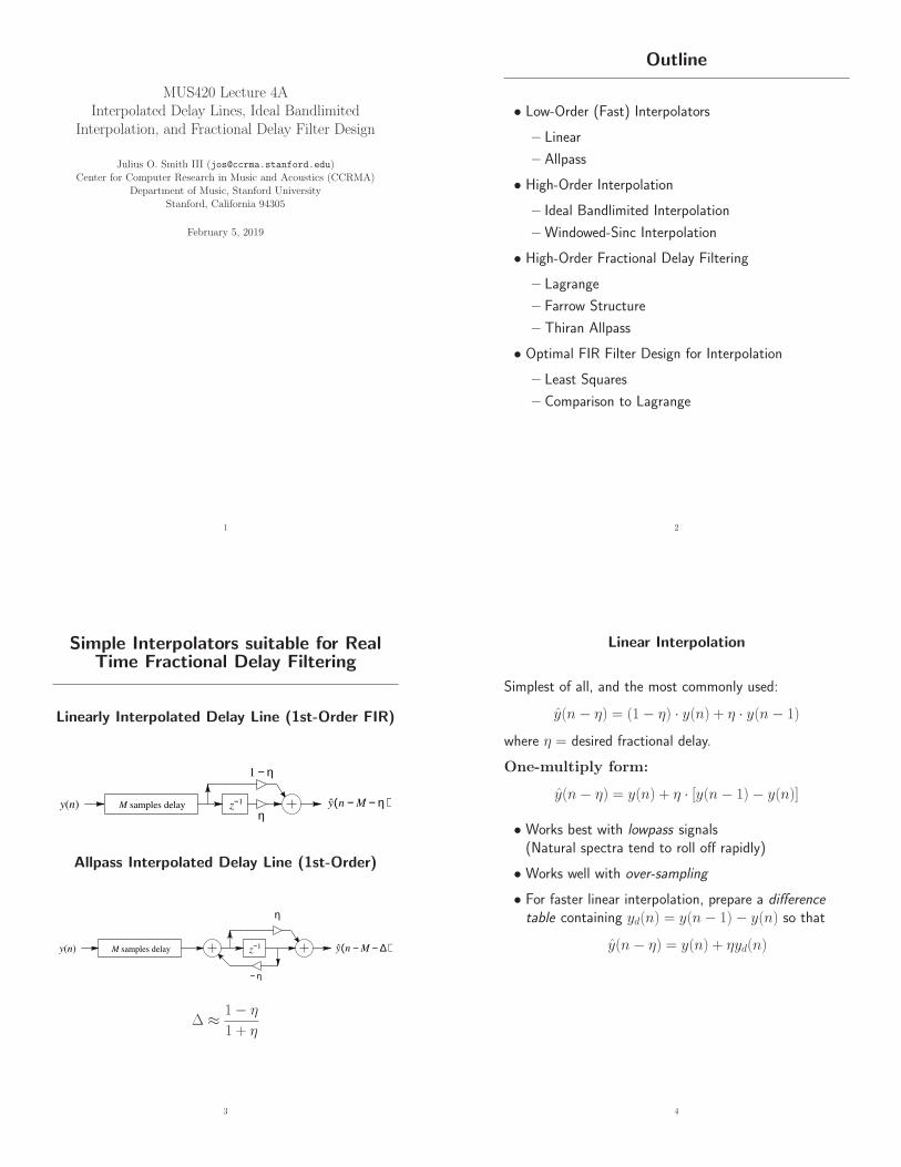
MUS420 Lecture 4A Interpolated Delay Lines, Ideal Bandlimited Interpolation, and Fractional Delay Filter Design Julius O. Smith III ([email protected]) Center for Computer Research in Music and Acoustics (CCRMA) Department of Music, Stanford University Stanford, California 94305 February 5, 2019 1 Outline • Low-Order (Fast) Interpolators – Linear – Allpass • High-Order Interpolation – Ideal Bandlimited Interpolation – Windowed-Sinc Interpolation • High-Order Fractional Delay Filtering – Lagrange – Farrow Structure – Thiran Allpass • Optimal FIR Filter Design for Interpolation – Least Squares – Comparison to Lagrange 2 Simple Interpolators suitable for Real Time Fractional Delay Filtering Linearly Interpolated Delay Line (1st-Order FIR) M samples delay z -1 η 1 η - y(n) ( 29 M n y ˆ η - - Allpass Interpolated Delay Line (1st-Order) M samples delay z -1 y(n) η η - ( 29 M n y ˆ ∆ - - ∆ ≈ 1 − η 1+ η 3 Linear Interpolation Simplest of all, and the most commonly used: ˆ y(n − η) = (1 − η) · y(n)+ η · y(n − 1) where η = desired fractional delay. One-multiply form: ˆ y(n − η)= y(n)+ η · [y(n − 1) − y(n)] • Works best with lowpass signals (Natural spectra tend to roll off rapidly) • Works well with over-sampling • For faster linear interpolation, prepare a difference table containing y d (n)= y(n − 1) − y(n) so that ˆ y(n − η)= y(n)+ ηy d (n) 4
Transcript of Outline Simple Interpolators suitable for Real Time Fractional Delay Filtering
MUS420 Lecture 4AInterpolated Delay Lines, Ideal Bandlimited
Interpolation, and Fractional Delay Filter Design
Julius O. Smith III ([email protected])Center for Computer Research in Music and Acoustics (CCRMA)
Department of Music, Stanford UniversityStanford, California 94305
February 5, 2019
1
Outline
• Low-Order (Fast) Interpolators
– Linear
– Allpass
• High-Order Interpolation
– Ideal Bandlimited Interpolation
– Windowed-Sinc Interpolation
• High-Order Fractional Delay Filtering
– Lagrange
– Farrow Structure
– Thiran Allpass
• Optimal FIR Filter Design for Interpolation
– Least Squares
– Comparison to Lagrange
2
Simple Interpolators suitable for RealTime Fractional Delay Filtering
Linearly Interpolated Delay Line (1st-Order FIR)
M samples delay z−1
η
1 η−
y(n) ( )Mny η−−
Allpass Interpolated Delay Line (1st-Order)
M samples delay z−1y(n)
η
η−
( )Mny ∆−−
∆ ≈1− η
1 + η
3
Linear Interpolation
Simplest of all, and the most commonly used:
y(n− η) = (1− η) · y(n) + η · y(n− 1)
where η = desired fractional delay.
One-multiply form:
y(n− η) = y(n) + η · [y(n− 1)− y(n)]
• Works best with lowpass signals(Natural spectra tend to roll off rapidly)
• Works well with over-sampling
• For faster linear interpolation, prepare a difference
table containing yd(n) = y(n− 1)− y(n) so that
y(n− η) = y(n) + ηyd(n)
4
Deriving Linear Interpolation from Taylor Series
Truncate a Taylor series expansion to first order and plugin a first-order derivative approximation:
y(n + α) = y(n) + α y(n) + α2 y(n)
2!+ α3
...y (n)
3!+ · · ·
≈ y(n) + α y(n)
⇒ y(n + α)∆= y(n) + α
y(n + 1)− y(n)
1
= α y(n + 1) + (1− α) y(n)
where α = −η = fractional advance desired(interpolation time between samples n and n + 1)
• Same approach can be used to define higher-orderinterpolation filters using various choices ofhigher-order derivative approximations
• Recall the many finite-difference schemes we have
5
Examples
Half-sample delay:
y
(
n−1
2
)
=1
2· y(n) +
1
2· y(n− 1)
Quarter-sample delay:
y
(
n−1
4
)
=3
4· y(n) +
1
4· y(n− 1)
6
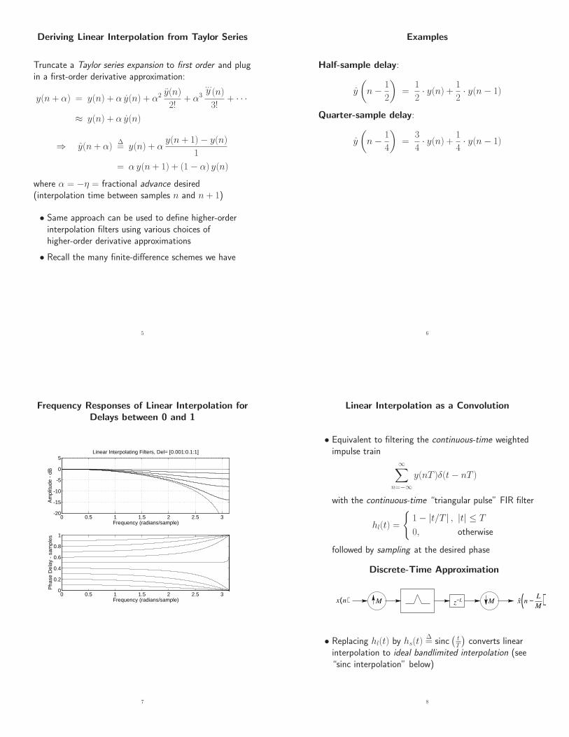
Frequency Responses of Linear Interpolation forDelays between 0 and 1
0 0.5 1 1.5 2 2.5 3-20
-15
-10
-5
0
5Linear Interpolating Filters, Del= [0.001:0.1:1]
Frequency (radians/sample)
Am
plitu
de -
dB
0 0.5 1 1.5 2 2.5 30
0.2
0.4
0.6
0.8
1
Frequency (radians/sample)
Pha
se D
elay
- s
ampl
es
7
Linear Interpolation as a Convolution
• Equivalent to filtering the continuous-time weightedimpulse train
∞∑
n=−∞
y(nT )δ(t− nT )
with the continuous-time “triangular pulse” FIR filter
hl(t) =
1− |t/T | , |t| ≤ T
0, otherwise
followed by sampling at the desired phase
Discrete-Time Approximation
z−LM M ( )M
Lnx −( )nx
• Replacing hl(t) by hs(t)∆= sinc
(
tT
)
converts linearinterpolation to ideal bandlimited interpolation (see“sinc interpolation” below)
8
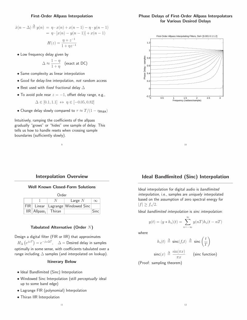
First-Order Allpass Interpolation
x(n−∆)∆= y(n) = η · x(n) + x(n− 1)− η · y(n− 1)
= η · [x(n)− y(n− 1)] + x(n− 1)
H(z) =η + z−1
1 + ηz−1
• Low frequency delay given by
∆ ≈1− η
1 + η(exact at DC)
• Same complexity as linear interpolation
• Good for delay-line interpolation, not random access
• Best used with fixed fractional delay ∆
• To avoid pole near z = −1, offset delay range, e.g.,
∆ ∈ [0.1, 1.1] ↔ η ∈ [−0.05, 0.82]
• Change delay slowly compared to τ ≈ T/(1− ηmax)
Intuitively, ramping the coefficients of the allpassgradually “grows” or “hides” one sample of delay. Thistells us how to handle resets when crossing sampleboundaries (sufficiently slowly).
9
Phase Delays of First-Order Allpass Interpolatorsfor Various Desired Delays
0 0.5 1 1.5 2 2.5 3-0.2
0
0.2
0.4
0.6
0.8
1
1.2
First-Order Allpass Interpolating Filters, Del= [0.001:0.1:1.2]
Frequency (radians/sample)
Pha
se D
elay
- s
ampl
es10
Interpolation Overview
Well Known Closed-Form Solutions
Order
1 N Large N ∞
FIR Linear Lagrange Windowed SincIIR Allpass1 Thiran Sinc
Tabulated Alternative (Order N)
Design a digital filter (FIR or IIR) that approximates
H∆
(
ejωT)
= e−jω∆T , ∆ = Desired delay in samples
optimally in some sense, with coefficients tabulated over arange including ∆ samples (and interpolated on lookup).
Itinerary Below
• Ideal Bandlimited (Sinc) Interpolation
• Windowed Sinc Interpolation (still perceptually idealup to some band edge)
• Lagrange FIR (polynomial) Interpolation
• Thiran IIR Interpolation
11
Ideal Bandlimited (Sinc) Interpolation
Ideal interpolation for digital audio is bandlimitedinterpolation, i.e., samples are uniquely interpolatedbased on the assumption of zero spectral energy for|f | ≥ fs/2.
Ideal bandlimited interpolation is sinc interpolation:
y(t) = (y ∗ hs)(t) =∞∑
n=−∞
y(nT )hs(t− nT )
where
hs(t)∆= sinc(fst)
∆= sinc
(
t
T
)
sinc(x)∆=
sin(πx)
πx(sinc function)
(Proof: sampling theorem)
12
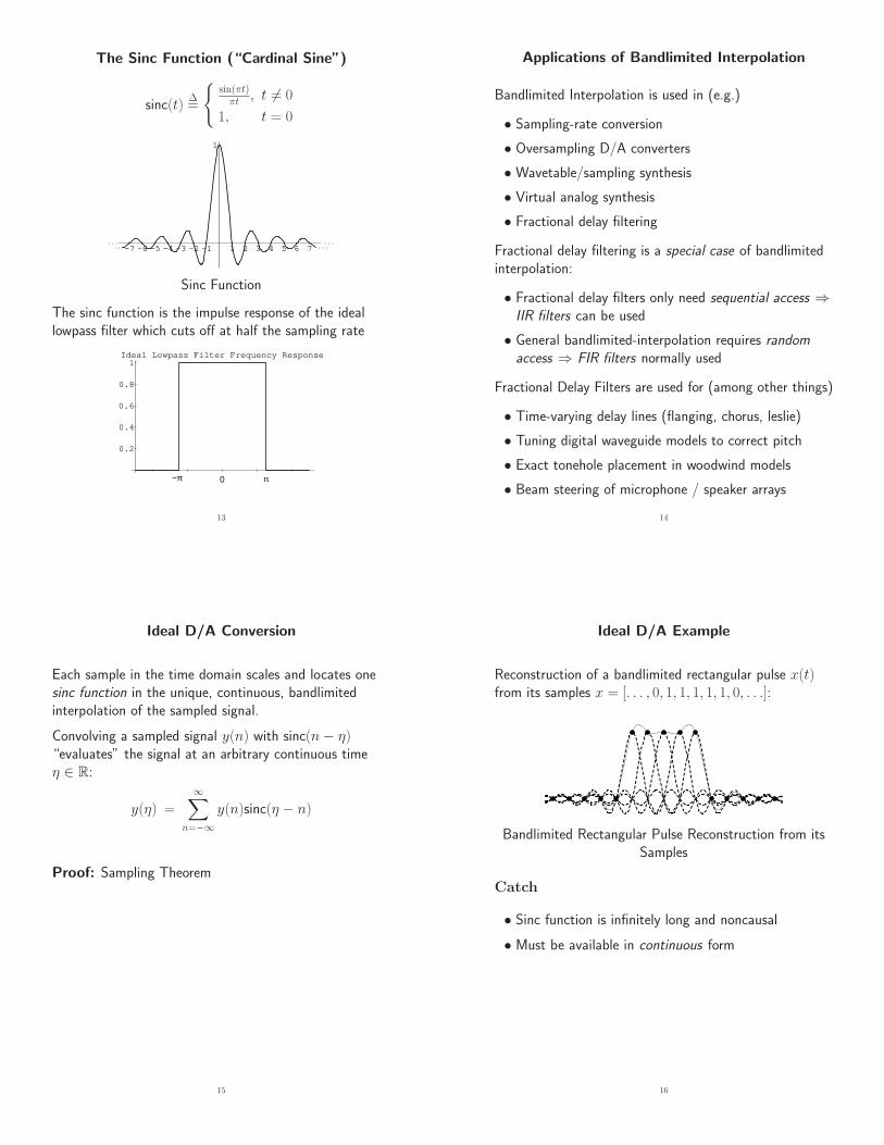
The Sinc Function (“Cardinal Sine”)
sinc(t)∆=
sin(πt)πt , t 6= 0
1, t = 0
-7 -6 -5 -4 -3 -2 -1 1 2 3 4 5 6 7
1
. . .. . .
. . .. . .
Sinc Function
The sinc function is the impulse response of the ideallowpass filter which cuts off at half the sampling rate
Ideal Lowpass Filter Frequency Response
0.2
0.4
0.6
0.8
1
π−π 0
13
Applications of Bandlimited Interpolation
Bandlimited Interpolation is used in (e.g.)
• Sampling-rate conversion
• Oversampling D/A converters
• Wavetable/sampling synthesis
• Virtual analog synthesis
• Fractional delay filtering
Fractional delay filtering is a special case of bandlimitedinterpolation:
• Fractional delay filters only need sequential access ⇒IIR filters can be used
• General bandlimited-interpolation requires randomaccess ⇒ FIR filters normally used
Fractional Delay Filters are used for (among other things)
• Time-varying delay lines (flanging, chorus, leslie)
• Tuning digital waveguide models to correct pitch
• Exact tonehole placement in woodwind models
• Beam steering of microphone / speaker arrays
14
Ideal D/A Conversion
Each sample in the time domain scales and locates onesinc function in the unique, continuous, bandlimitedinterpolation of the sampled signal.
Convolving a sampled signal y(n) with sinc(n− η)“evaluates” the signal at an arbitrary continuous timeη ∈ R:
y(η) =
∞∑
n=−∞
y(n)sinc(η − n)
Proof: Sampling Theorem
15
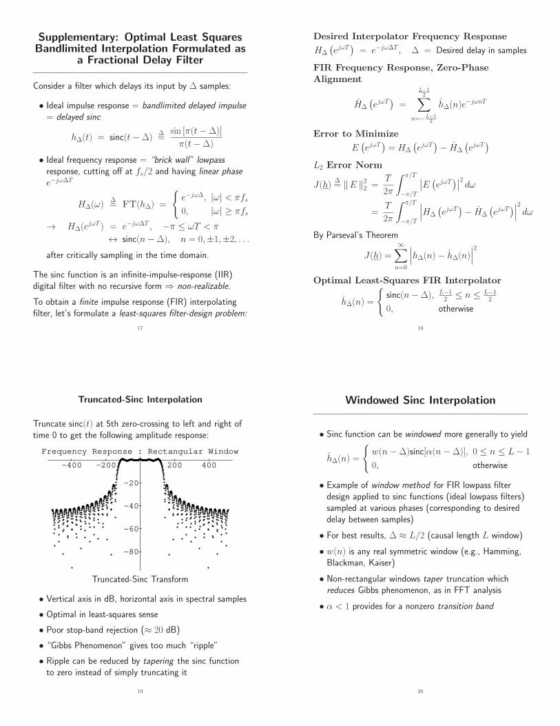
Ideal D/A Example
Reconstruction of a bandlimited rectangular pulse x(t)from its samples x = [. . . , 0, 1, 1, 1, 1, 1, 0, . . .]:
Bandlimited Rectangular Pulse Reconstruction from itsSamples
Catch
• Sinc function is infinitely long and noncausal
• Must be available in continuous form
16
Supplementary: Optimal Least SquaresBandlimited Interpolation Formulated as
a Fractional Delay Filter
Consider a filter which delays its input by ∆ samples:
• Ideal impulse response = bandlimited delayed impulse
= delayed sinc
h∆(t) = sinc(t−∆)∆=
sin [π(t−∆)]
π(t−∆)
• Ideal frequency response = “brick wall” lowpass
response, cutting off at fs/2 and having linear phase
e−jω∆T
H∆(ω)∆= FT(h∆) =
e−jω∆, |ω| < πfs
0, |ω| ≥ πfs
→ H∆(ejωT ) = e−jω∆T , −π ≤ ωT < π
↔ sinc(n−∆), n = 0,±1,±2, . . .
after critically sampling in the time domain.
The sinc function is an infinite-impulse-response (IIR)digital filter with no recursive form ⇒ non-realizable.
To obtain a finite impulse response (FIR) interpolatingfilter, let’s formulate a least-squares filter-design problem:
17
Desired Interpolator Frequency Response
H∆
(
ejωT)
= e−jω∆T , ∆ = Desired delay in samples
FIR Frequency Response, Zero-PhaseAlignment
H∆
(
ejωT)
=
L−12
∑
n=−L−12
h∆(n)e−jωnT
Error to Minimize
E(
ejωT)
= H∆
(
ejωT)
− H∆
(
ejωT)
L2 Error Norm
J(h)∆= ‖E ‖22 =
T
2π
∫ π/T
−π/T
∣
∣E(
ejωT)∣
∣
2dω
=T
2π
∫ π/T
−π/T
∣
∣
∣H∆
(
ejωT)
− H∆
(
ejωT)
∣
∣
∣
2
dω
By Parseval’s Theorem
J(h) =
∞∑
n=0
∣
∣
∣h∆(n)− h∆(n)
∣
∣
∣
2
Optimal Least-Squares FIR Interpolator
h∆(n) =
sinc(n−∆), L−12 ≤ n ≤ L−1
2
0, otherwise
18
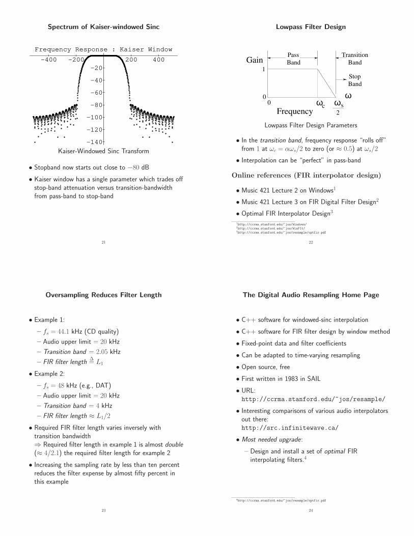
Truncated-Sinc Interpolation
Truncate sinc(t) at 5th zero-crossing to left and right oftime 0 to get the following amplitude response:
Frequency Response : Rectangular Window
-400 -200 200 400
-80
-60
-40
-20
Truncated-Sinc Transform
• Vertical axis in dB, horizontal axis in spectral samples
• Optimal in least-squares sense
• Poor stop-band rejection (≈ 20 dB)
• “Gibbs Phenomenon” gives too much “ripple”
• Ripple can be reduced by tapering the sinc functionto zero instead of simply truncating it
19
Windowed Sinc Interpolation
• Sinc function can be windowed more generally to yield
h∆(n) =
w(n−∆)sinc[α(n−∆)], 0 ≤ n ≤ L− 1
0, otherwise
• Example of window method for FIR lowpass filterdesign applied to sinc functions (ideal lowpass filters)sampled at various phases (corresponding to desireddelay between samples)
• For best results, ∆ ≈ L/2 (causal length L window)
• w(n) is any real symmetric window (e.g., Hamming,Blackman, Kaiser)
• Non-rectangular windows taper truncation whichreduces Gibbs phenomenon, as in FFT analysis
• α < 1 provides for a nonzero transition band
20
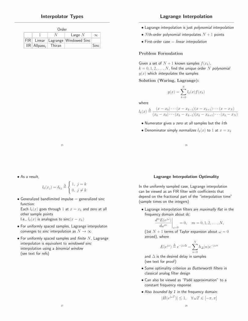
Spectrum of Kaiser-windowed Sinc
Frequency Response : Kaiser Window
-400 -200 200 400
-140
-120
-100
-80
-60
-40
-20
Kaiser-Windowed Sinc Transform
• Stopband now starts out close to −80 dB
• Kaiser window has a single parameter which trades offstop-band attenuation versus transition-bandwidthfrom pass-band to stop-band
21
Lowpass Filter Design
ω
Gain
ωc0
0
1
ωs
2
Transition
Band
Pass
Band
Stop
Band
Frequency
Lowpass Filter Design Parameters
• In the transition band, frequency response “rolls off”from 1 at ωc = αωs/2 to zero (or ≈ 0.5) at ωs/2
• Interpolation can be “perfect” in pass-band
Online references (FIR interpolator design)
• Music 421 Lecture 2 on Windows1
• Music 421 Lecture 3 on FIR Digital Filter Design2
• Optimal FIR Interpolator Design3
1http://ccrma.stanford.edu/~jos/Windows/2http://ccrma.stanford.edu/~jos/WinFlt/3http://ccrma.stanford.edu/~jos/resample/optfir.pdf
22
Oversampling Reduces Filter Length
• Example 1:
– fs = 44.1 kHz (CD quality)
– Audio upper limit = 20 kHz
– Transition band = 2.05 kHz
– FIR filter length∆= L1
• Example 2:
– fs = 48 kHz (e.g., DAT)
– Audio upper limit = 20 kHz
– Transition band = 4 kHz
– FIR filter length ≈ L1/2
• Required FIR filter length varies inversely withtransition bandwidth⇒ Required filter length in example 1 is almost double(≈ 4/2.1) the required filter length for example 2
• Increasing the sampling rate by less than ten percentreduces the filter expense by almost fifty percent inthis example
23
The Digital Audio Resampling Home Page
• C++ software for windowed-sinc interpolation
• C++ software for FIR filter design by window method
• Fixed-point data and filter coefficients
• Can be adapted to time-varying resampling
• Open source, free
• First written in 1983 in SAIL
• URL:http://ccrma.stanford.edu/~jos/resample/
• Interesting comparisons of various audio interpolatorsout there:http://src.infinitewave.ca/
• Most needed upgrade:
– Design and install a set of optimal FIRinterpolating filters.4
4http://ccrma.stanford.edu/~jos/resample/optfir.pdf
24
Interpolator Types
Order
1 N Large N ∞
FIR Linear Lagrange Windowed SincIIR Allpass1 Thiran Sinc
25
Lagrange Interpolation
• Lagrange interpolation is just polynomial interpolation
• N th-order polynomial interpolates N + 1 points
• First-order case = linear interpolation
Problem Formulation
Given a set of N + 1 known samples f (xk),k = 0, 1, 2, . . . , N , find the unique order N polynomial
y(x) which interpolates the samples
Solution (Waring, Lagrange):
y(x) =N∑
k=0
lk(x)f (xk)
where
lk(x)∆=
(x− x0) · · · (x− xk−1)(x− xk+1) · · · (x− xN)
(xk − x0) · · · (xk − xk−1)(xk − xk+1) · · · (xk − xN)
• Numerator gives a zero at all samples but the kth
• Denominator simply normalizes lk(x) to 1 at x = xk
26
• As a result,
lk(xj) = δkj∆=
1, j = k
0, j 6= k
• Generalized bandlimited impulse = generalized sincfunction:Each lk(x) goes through 1 at x = xk and zero at allother sample pointsI.e., lk(x) is analogous to sinc(x− xk)
• For uniformly spaced samples, Lagrange interpolatonconverges to sinc interpolation as N →∞
• For uniformly spaced samples and finite N , Lagrangeinterpolaton is equivalent to windowed sinc
interpolation using a binomial window
(see text for refs)
27
Lagrange Interpolation Optimality
In the uniformly sampled case, Lagrange interpolationcan be viewed as an FIR filter with coefficients thatdepend on the fractional part of the “interpolation time”(sample times on the integers)
• Lagrange interpolation filters are maximally flat in thefrequency domain about dc:
dmE(ejω)
dωm
∣
∣
∣
∣
ω=0
= 0, m = 0, 1, 2, . . . , N,
(1st N + 1 terms of Taylor expansion about ω = 0zeroed), where
E(ejω)∆= e−jω∆ −
N∑
n=0
h∆(n)e−jωn
and ∆ is the desired delay in samples(see text for proof)
• Same optimality criterion as Butterworth filters inclassical analog filter design
• Can also be viewed as “Pade approximation” to aconstant frequency response
• Also bounded by 1 in the frequency domain:
|H(ejωT )| ≤ 1, ∀ωT ∈ [−π, π]
28
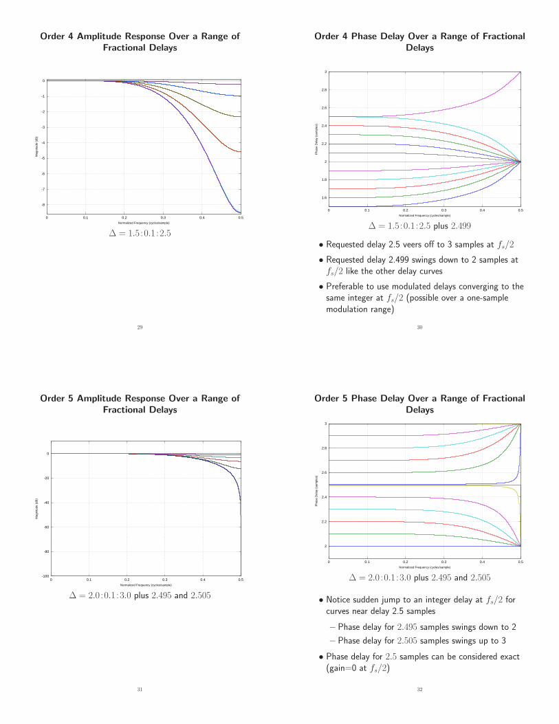
Order 4 Amplitude Response Over a Range ofFractional Delays
-8
-7
-6
-5
-4
-3
-2
-1
0
0 0.1 0.2 0.3 0.4 0.5
Mag
nitu
de (
dB)
Normalized Frequency (cycles/sample)
∆ = 1.5 :0.1 :2.5
29
Order 4 Phase Delay Over a Range of FractionalDelays
1.6
1.8
2
2.2
2.4
2.6
2.8
3
0 0.1 0.2 0.3 0.4 0.5
Pha
se D
elay
(sa
mpl
es)
Normalized Frequency (cycles/sample)
∆ = 1.5 :0.1 :2.5 plus 2.499
• Requested delay 2.5 veers off to 3 samples at fs/2
• Requested delay 2.499 swings down to 2 samples atfs/2 like the other delay curves
• Preferable to use modulated delays converging to thesame integer at fs/2 (possible over a one-samplemodulation range)
30
Order 5 Amplitude Response Over a Range ofFractional Delays
-100
-80
-60
-40
-20
0
0 0.1 0.2 0.3 0.4 0.5
Mag
nitu
de (
dB)
Normalized Frequency (cycles/sample)
∆ = 2.0 :0.1 :3.0 plus 2.495 and 2.505
31
Order 5 Phase Delay Over a Range of FractionalDelays
2
2.2
2.4
2.6
2.8
3
0 0.1 0.2 0.3 0.4 0.5
Pha
se D
elay
(sa
mpl
es)
Normalized Frequency (cycles/sample)
∆ = 2.0 :0.1 :3.0 plus 2.495 and 2.505
• Notice sudden jump to an integer delay at fs/2 forcurves near delay 2.5 samples
– Phase delay for 2.495 samples swings down to 2
– Phase delay for 2.505 samples swings up to 3
• Phase delay for 2.5 samples can be considered exact(gain=0 at fs/2)
32
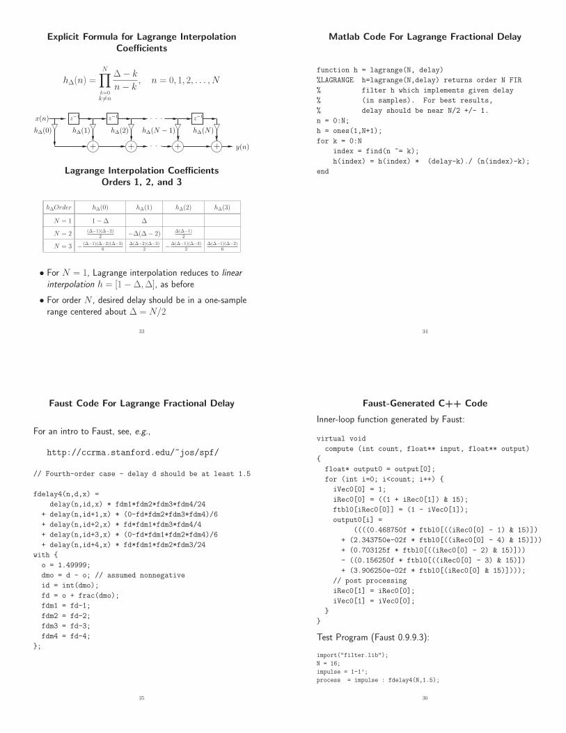
Explicit Formula for Lagrange InterpolationCoefficients
h∆(n) =
N∏
k=0k 6=n
∆− k
n− k, n = 0, 1, 2, . . . , N
y(n)
h∆(N)h∆(0)
. . .
h∆(1) h∆(2)
. . .
h∆(N − 1)
x(n) z−1 z−1z−1
Lagrange Interpolation CoefficientsOrders 1, 2, and 3
h∆Order h∆(0) h∆(1) h∆(2) h∆(3)
N = 1 1−∆ ∆
N = 2 (∆−1)(∆−2)2 −∆(∆− 2) ∆(∆−1)
2
N = 3 − (∆−1)(∆−2)(∆−3)6
∆(∆−2)(∆−3)2 −∆(∆−1)(∆−3)
2∆(∆−1)(∆−2)
6
• For N = 1, Lagrange interpolation reduces to linear
interpolation h = [1−∆,∆], as before
• For order N , desired delay should be in a one-samplerange centered about ∆ = N/2
33
Matlab Code For Lagrange Fractional Delay
function h = lagrange(N, delay)
%LAGRANGE h=lagrange(N,delay) returns order N FIR
% filter h which implements given delay
% (in samples). For best results,
% delay should be near N/2 +/- 1.
n = 0:N;
h = ones(1,N+1);
for k = 0:N
index = find(n ~= k);
h(index) = h(index) * (delay-k)./ (n(index)-k);
end
34
Faust Code For Lagrange Fractional Delay
For an intro to Faust, see, e.g.,
http://ccrma.stanford.edu/~jos/spf/
// Fourth-order case - delay d should be at least 1.5
fdelay4(n,d,x) =
delay(n,id,x) * fdm1*fdm2*fdm3*fdm4/24
+ delay(n,id+1,x) * (0-fd*fdm2*fdm3*fdm4)/6
+ delay(n,id+2,x) * fd*fdm1*fdm3*fdm4/4
+ delay(n,id+3,x) * (0-fd*fdm1*fdm2*fdm4)/6
+ delay(n,id+4,x) * fd*fdm1*fdm2*fdm3/24
with
o = 1.49999;
dmo = d - o; // assumed nonnegative
id = int(dmo);
fd = o + frac(dmo);
fdm1 = fd-1;
fdm2 = fd-2;
fdm3 = fd-3;
fdm4 = fd-4;
;
35
Faust-Generated C++ Code
Inner-loop function generated by Faust:
virtual void
compute (int count, float** input, float** output)
float* output0 = output[0];
for (int i=0; i<count; i++)
iVec0[0] = 1;
iRec0[0] = ((1 + iRec0[1]) & 15);
ftbl0[iRec0[0]] = (1 - iVec0[1]);
output0[i] =
((((0.468750f * ftbl0[((iRec0[0] - 1) & 15)])
+ (2.343750e-02f * ftbl0[((iRec0[0] - 4) & 15)]))
+ (0.703125f * ftbl0[((iRec0[0] - 2) & 15)]))
- ((0.156250f * ftbl0[((iRec0[0] - 3) & 15)])
+ (3.906250e-02f * ftbl0[(iRec0[0] & 15)])));
// post processing
iRec0[1] = iRec0[0];
iVec0[1] = iVec0[0];
Test Program (Faust 0.9.9.3):
import("filter.lib");
N = 16;
impulse = 1-1’;
process = impulse : fdelay4(N,1.5);
36
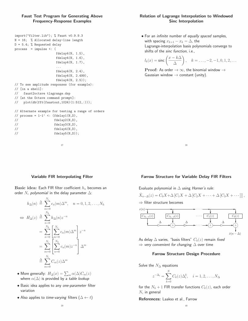
Faust Test Program for Generating AboveFrequency-Response Examples
import("filter.lib"); % Faust v0.9.9.3
N = 16; % Allocated delay-line length
D = 5.4; % Requested delay
process = impulse <: (
fdelay4(N, 1.5),
fdelay4(N, 1.6),
fdelay4(N, 1.7),
...
fdelay4(N, 2.4),
fdelay4(N, 2.499),
fdelay4(N, 2.5));
// To see amplitude responses (for example):
// [in a shell]:
// faust2octave tlagrange.dsp
// [at the Octave command prompt]:
// plot(db(fft(faustout,1024)(1:512,:)));
// Alternate example for testing a range of orders
// process = 1-1’ <: (fdelay1(N,D),
// fdelay2(N,D),
// fdelay3(N,D),
// fdelay4(N,D),
// fdelay5(N,D));
37
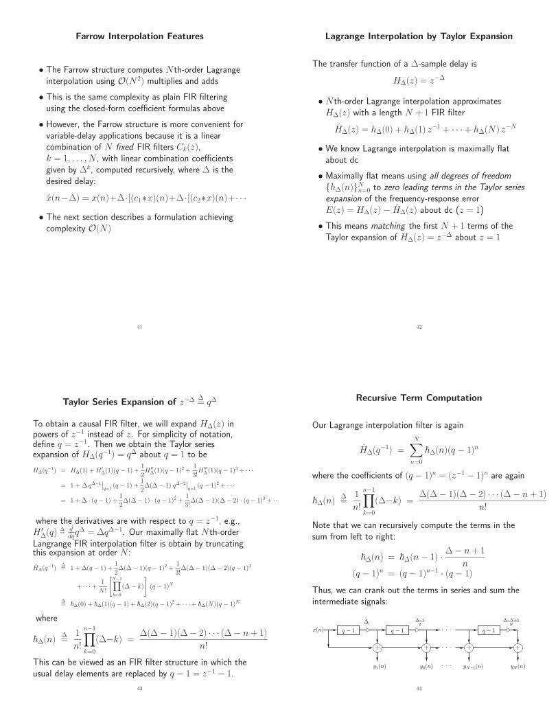
Relation of Lagrange Interpolation to WindowedSinc Interpolation
• For an infinite number of equally spaced samples,with spacing xk+1 − xk = ∆, theLagrange-interpolation basis polynomials converge toshifts of the sinc function, i.e.,
lk(x) = sinc
(
x− k∆
∆
)
, k = . . . ,−2,−1, 0, 1, 2, . . .
Proof: As order →∞, the binomial window →Gaussian window → constant (unity).
38
Variable FIR Interpolating Filter
Basic idea: Each FIR filter coefficient hn becomes anorder Nc polynomial in the delay parameter ∆:
h∆(n)∆=
Nc∑
m=0
cn(m)∆m, n = 0, 1, 2, . . . , Nh
⇔ H∆(z)∆=
Nh∑
n=0
h∆(n)z−n
=
Nh∑
n=0
[
Nc∑
m=0
cn(m)∆m
]
z−n
=
Nc∑
m=0
Nh∑
n=0
cn(m)z−n
∆m
∆=
Nc∑
m=0
Cm(z)∆m
• More generally: H∆(x) =∑
m α(∆)Cm(z)where α(∆) is provided by a table lookup
• Basic idea applies to any one-parameter filtervariation
• Also applies to time-varying filters (∆← t)
39
Farrow Structure for Variable Delay FIR Filters
Evaluate polynomial in ∆ using Horner’s rule:
Xn−∆(z) = C0X+∆ [C1X +∆ [C2X + · · · +∆ [C3X + · · · ]]] ,
⇒ filter structure becomes
. . .
x(n−∆)
x(n) . . .
. . .
∆
CNc−1(z)
∆
CNc−2(z) C0(z)C1(z)
∆
As delay ∆ varies, “basis filters” Ck(z) remain fixed
⇒ very convenient for changing ∆ over time
Farrow Structure Design Procedure
Solve the N∆ equations
z−∆i =
N∑
k=0
Ck(z)∆ki , i = 1, 2, . . . , N∆
for the Nh + 1 FIR transfer functions Ck(z), each orderNc in general
References: Laakso et al., Farrow
40
Farrow Interpolation Features
• The Farrow structure computes N th-order Lagrangeinterpolation using O(N 2) multiplies and adds
• This is the same complexity as plain FIR filteringusing the closed-form coefficient formulas above
• However, the Farrow structure is more convenient forvariable-delay applications because it is a linearcombination of N fixed FIR filters Ck(z),k = 1, . . . , N , with linear combination coefficientsgiven by ∆k, computed recursively, where ∆ is thedesired delay:
x(n−∆) = x(n)+∆·[(c1∗x)(n)+∆·[(c2∗x)(n)+· · ·
• The next section describes a formulation achievingcomplexity O(N)
41
Lagrange Interpolation by Taylor Expansion
The transfer function of a ∆-sample delay is
H∆(z) = z−∆
• N th-order Lagrange interpolation approximatesH∆(z) with a length N + 1 FIR filter
H∆(z) = h∆(0) + h∆(1) z−1 + · · · + h∆(N) z−N
• We know Lagrange interpolation is maximally flatabout dc
• Maximally flat means using all degrees of freedom
h∆(n)Nn=0 to zero leading terms in the Taylor series
expansion of the frequency-response errorE(z) = H∆(z)− H∆(z) about dc (z = 1)
• This means matching the first N + 1 terms of theTaylor expansion of H∆(z) = z−∆ about z = 1
42
Taylor Series Expansion of z−∆∆= q∆
To obtain a causal FIR filter, we will expand H∆(z) inpowers of z−1 instead of z. For simplicity of notation,define q = z−1. Then we obtain the Taylor seriesexpansion of H∆(q
−1) = q∆ about q = 1 to be
H∆(q−1) = H∆(1) +H ′∆(1)(q − 1) +
1
2H ′′∆(1)(q − 1)2 +
1
3!H ′′′∆(1)(q − 1)3 + · · ·
= 1 + ∆ q∆−1∣
∣
q=1(q − 1) +
1
2∆(∆− 1) q∆−2
∣
∣
q=1(q − 1)2 + · · ·
= 1 +∆ · (q − 1) +1
2∆(∆− 1) · (q − 1)2 +
1
3!∆(∆− 1)(∆− 2) · (q − 1)3 + · · ·
where the derivatives are with respect to q = z−1, e.g.,H ′∆(q)
∆=
ddqq
∆ = ∆q∆−1. Our maximally flat N th-orderLangrange FIR interpolation filter is obtain by truncatingthis expansion at order N :
H∆(q−1)
∆= 1 +∆(q − 1) +
1
2∆(∆− 1)(q − 1)2 +
1
3!∆(∆− 1)(∆− 2)(q − 1)3
+ · · ·+1
N !
[
N−1∏
k=0
(∆− k)
]
(q − 1)N
∆= ~∆(0) + ~∆(1)(q − 1) + ~∆(2)(q − 1)2 + · · ·+ ~∆(N)(q − 1)N
where
~∆(n)∆=
1
n!
n−1∏
k=0
(∆−k) =∆(∆− 1)(∆− 2) · · · (∆− n + 1)
n!
This can be viewed as an FIR filter structure in which theusual delay elements are replaced by q − 1 = z−1 − 1.
43
Recursive Term Computation
Our Lagrange interpolation filter is again
H∆(q−1) =
N∑
n=0
~∆(n)(q − 1)n
where the coefficients of (q − 1)n = (z−1 − 1)n are again
~∆(n)∆=
1
n!
n−1∏
k=0
(∆−k) =∆(∆− 1)(∆− 2) · · · (∆− n + 1)
n!
Note that we can recursively compute the terms in thesum from left to right:
~∆(n) = ~∆(n− 1) ·∆− n + 1
n(q − 1)n = (q − 1)n−1 · (q − 1)
Thus, we can crank out the terms in series and sum theintermediate signals:
. . . yN−1(n) yN(n)
∆−N+1
N∆
y1(n) y2(n)
∆−1
2
. . .
. . .
x(n) q − 1q − 1q − 1
44
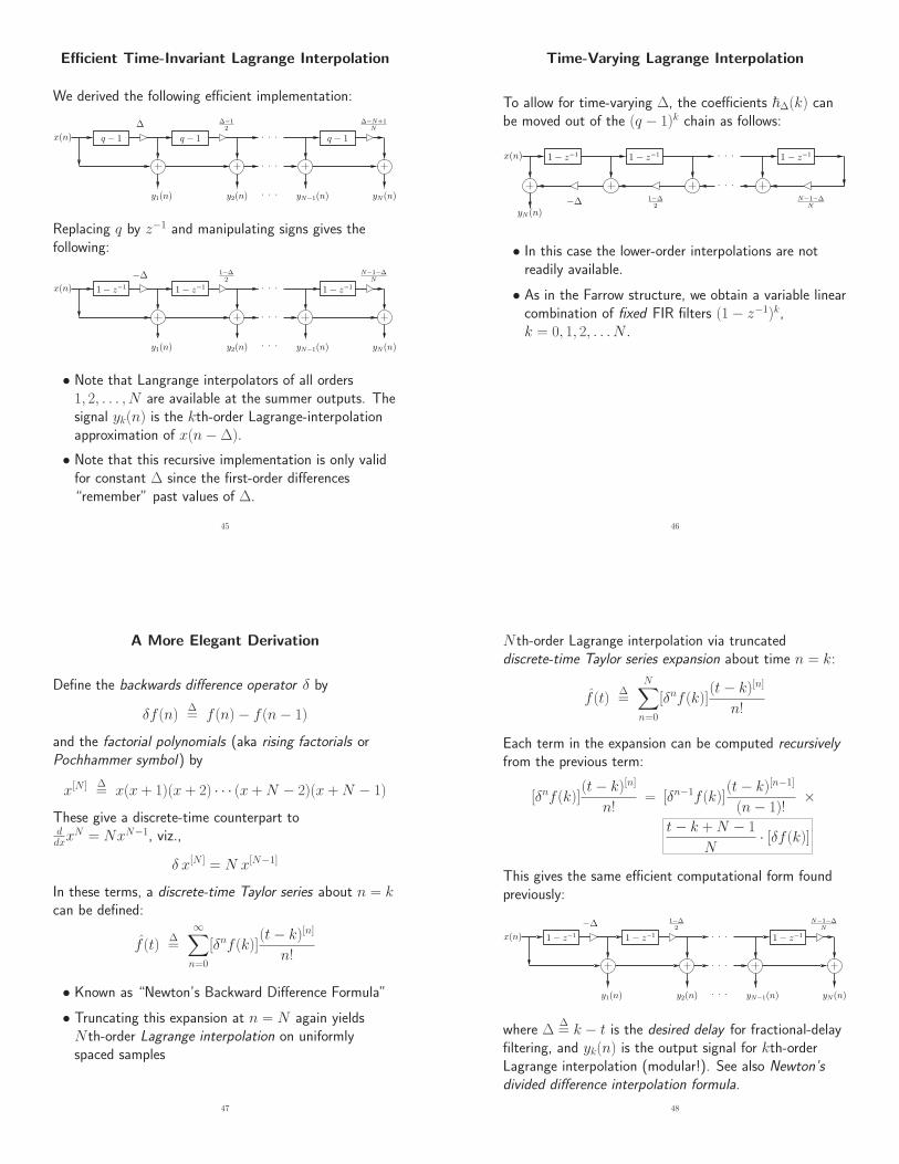
Efficient Time-Invariant Lagrange Interpolation
We derived the following efficient implementation:
. . . yN−1(n) yN(n)
∆−N+1
N∆
y1(n) y2(n)
∆−1
2
. . .
. . .
x(n) q − 1q − 1q − 1
Replacing q by z−1 and manipulating signs gives thefollowing:
. . . yN−1(n) yN(n)
N−1−∆
N−∆
y1(n) y2(n)
1−∆
2
. . .
. . .
x(n) 1− z−11− z−11− z−1
• Note that Langrange interpolators of all orders1, 2, . . . , N are available at the summer outputs. Thesignal yk(n) is the kth-order Lagrange-interpolationapproximation of x(n−∆).
• Note that this recursive implementation is only validfor constant ∆ since the first-order differences“remember” past values of ∆.
45
Time-Varying Lagrange Interpolation
To allow for time-varying ∆, the coefficients ~∆(k) canbe moved out of the (q − 1)k chain as follows:
x(n) . . .
. . .
N−1−∆
N
yN(n)−∆ 1−∆
2
1− z−11− z−1 1− z−1
• In this case the lower-order interpolations are notreadily available.
• As in the Farrow structure, we obtain a variable linearcombination of fixed FIR filters (1− z−1)k,k = 0, 1, 2, . . . N .
46
A More Elegant Derivation
Define the backwards difference operator δ by
δf (n)∆= f (n)− f (n− 1)
and the factorial polynomials (aka rising factorials orPochhammer symbol) by
x[N ] ∆= x(x + 1)(x + 2) · · · (x +N − 2)(x +N − 1)
These give a discrete-time counterpart toddxx
N = NxN−1, viz.,
δ x[N ] = N x[N−1]
In these terms, a discrete-time Taylor series about n = kcan be defined:
f (t)∆=
∞∑
n=0
[δnf (k)](t− k)[n]
n!
• Known as “Newton’s Backward Difference Formula”
• Truncating this expansion at n = N again yieldsN th-order Lagrange interpolation on uniformlyspaced samples
47
N th-order Lagrange interpolation via truncateddiscrete-time Taylor series expansion about time n = k:
f (t)∆=
N∑
n=0
[δnf (k)](t− k)[n]
n!
Each term in the expansion can be computed recursively
from the previous term:
[δnf (k)](t− k)[n]
n!= [δn−1f (k)]
(t− k)[n−1]
(n− 1)!×
t− k +N − 1
N· [δf (k)]
This gives the same efficient computational form foundpreviously:
. . . yN−1(n) yN(n)
N−1−∆
N−∆
y1(n) y2(n)
1−∆
2
. . .
. . .
x(n) 1− z−11− z−11− z−1
where ∆∆= k − t is the desired delay for fractional-delay
filtering, and yk(n) is the output signal for kth-orderLagrange interpolation (modular!). See also Newton’s
divided difference interpolation formula.
48
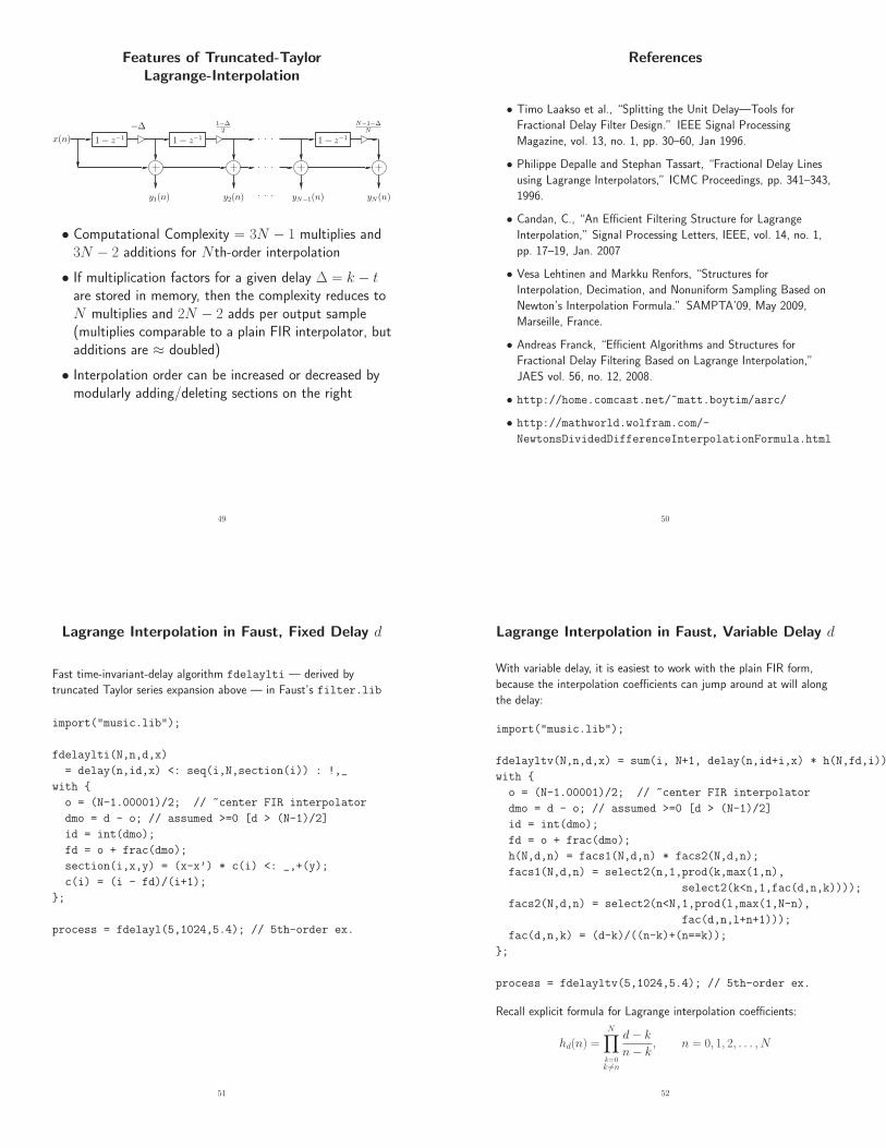
Features of Truncated-TaylorLagrange-Interpolation
. . . yN−1(n) yN(n)
N−1−∆
N−∆
y1(n) y2(n)
1−∆
2
. . .
. . .
x(n) 1− z−11− z−11− z−1
• Computational Complexity = 3N − 1 multiplies and3N − 2 additions for N th-order interpolation
• If multiplication factors for a given delay ∆ = k − tare stored in memory, then the complexity reduces toN multiplies and 2N − 2 adds per output sample(multiplies comparable to a plain FIR interpolator, butadditions are ≈ doubled)
• Interpolation order can be increased or decreased bymodularly adding/deleting sections on the right
49
References
• Timo Laakso et al., “Splitting the Unit Delay—Tools for
Fractional Delay Filter Design.” IEEE Signal Processing
Magazine, vol. 13, no. 1, pp. 30–60, Jan 1996.
• Philippe Depalle and Stephan Tassart, “Fractional Delay Lines
using Lagrange Interpolators,” ICMC Proceedings, pp. 341–343,
1996.
• Candan, C., “An Efficient Filtering Structure for Lagrange
Interpolation,” Signal Processing Letters, IEEE, vol. 14, no. 1,
pp. 17–19, Jan. 2007
• Vesa Lehtinen and Markku Renfors, “Structures for
Interpolation, Decimation, and Nonuniform Sampling Based on
Newton’s Interpolation Formula.” SAMPTA’09, May 2009,
Marseille, France.
• Andreas Franck, “Efficient Algorithms and Structures for
Fractional Delay Filtering Based on Lagrange Interpolation,”
JAES vol. 56, no. 12, 2008.
• http://home.comcast.net/~matt.boytim/asrc/
• http://mathworld.wolfram.com/-
NewtonsDividedDifferenceInterpolationFormula.html
50
Lagrange Interpolation in Faust, Fixed Delay d
Fast time-invariant-delay algorithm fdelaylti — derived by
truncated Taylor series expansion above — in Faust’s filter.lib
import("music.lib");
fdelaylti(N,n,d,x)
= delay(n,id,x) <: seq(i,N,section(i)) : !,_
with
o = (N-1.00001)/2; // ~center FIR interpolator
dmo = d - o; // assumed >=0 [d > (N-1)/2]
id = int(dmo);
fd = o + frac(dmo);
section(i,x,y) = (x-x’) * c(i) <: _,+(y);
c(i) = (i - fd)/(i+1);
;
process = fdelayl(5,1024,5.4); // 5th-order ex.
51
Lagrange Interpolation in Faust, Variable Delay d
With variable delay, it is easiest to work with the plain FIR form,
because the interpolation coefficients can jump around at will along
the delay:
import("music.lib");
fdelayltv(N,n,d,x) = sum(i, N+1, delay(n,id+i,x) * h(N,fd,i))
with
o = (N-1.00001)/2; // ~center FIR interpolator
dmo = d - o; // assumed >=0 [d > (N-1)/2]
id = int(dmo);
fd = o + frac(dmo);
h(N,d,n) = facs1(N,d,n) * facs2(N,d,n);
facs1(N,d,n) = select2(n,1,prod(k,max(1,n),
select2(k<n,1,fac(d,n,k))));
facs2(N,d,n) = select2(n<N,1,prod(l,max(1,N-n),
fac(d,n,l+n+1)));
fac(d,n,k) = (d-k)/((n-k)+(n==k));
;
process = fdelayltv(5,1024,5.4); // 5th-order ex.
Recall explicit formula for Lagrange interpolation coefficients:
hd(n) =N∏
k=0k 6=n
d− k
n− k, n = 0, 1, 2, . . . , N
52

Summary of Lagrange Interpolators Considered
y(n)
h∆(N)h∆(0)
. . .
h∆(1) h∆(2)
. . .
h∆(N − 1)
x(n) z−1 z−1z−1
Generic FIR
. . .
x(n−∆)
x(n) . . .
. . .
∆
CNc−1(z)
∆
CNc−2(z) C0(z)C1(z)
∆
Farrow Structure
. . . yN−1(n) yN(n)
N−1−∆
N−∆
y1(n) y2(n)
1−∆
2
. . .
. . .
x(n) 1− z−11− z−11− z−1
Truncated Taylor Expansion
53
Thiran Allpass Interpolators
Given a desired delay ∆ = N + δ samples, an order N allpass filter
H(z) =z−NA
(
z−1)
A(z)=
aN + aN−1z−1 + · · · + a1z
−(N−1) + z−N
1 + a1z−1 + · · · + aN−1z−(N−1) + aNz−N
can be designed having maximally flat group delay equal to ∆ at
DC using the formula
ak = (−1)k(
N
k
) N∏
n=0
∆−N + n
∆−N + k + n, k = 0, 1, 2, . . . , N
where(
N
k
)
=N !
k!(N − k)!
denotes the kth binomial coefficient
• a0 = 1 without further scaling
• For sufficiently large ∆, stability is guaranteed
rule of thumb: ∆ ≈ order
• Mean group delay is always N samples
(for any stable N th-order allpass filter):
1
2π
∫ 2π
0
D(ω)dω∆= −
1
2π
∫ 2π
0
Θ′(ω)dω = −1
2π[Θ(2π)− Θ(0)] = N
• Only known closed-form case for allpass interpolators of arbitrary
order
54
• Effective for delay-line interpolation needed for tuning since
pitch perception is most acute at low frequencies.
Frequency Responses of Thiran AllpassInterpolators for Fractional Delay
0 0.5 1 1.5 2 2.5 3 3.5−2
−1.5
−1
−0.5
0
0.5Thiran Interpolating Filters, Del=Order+0.3, Order=[1,2,3,5,10,20]
Gro
up D
elay
− s
ampl
es
Frequency (radians/sample)
1 2 3 5 1020
55
Large Delay Changes
When implementing large delay-length changes (by many samples), a
useful implementation is to cross-fade from the initial delay line
configuration to the new configuration.
• Computation doubled during cross-fade
• Cross-fade should be long enough to sound smooth
• Not a true “morph” from one delay length to another, since we
do not pass through the intermediate delay lengths.
• A single delay line can be shared such that the cross-fade occurs
from one read-pointer (plus associated filtering) to another.
56
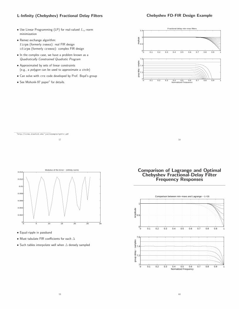
L-Infinity (Chebyshev) Fractional Delay Filters
• Use Linear Programming (LP) for real-valued L∞-norm
minimization
• Remez exchange algorithm:
firpm (formerly remez): real FIR design
cfirpm (formerly cremez): complex FIR design
• In the complex case, we have a problem known as a
Quadratically Constrained Quadratic Program
• Approximated by sets of linear constraints
(e.g., a polygon can be used to approximate a circle)
• Can solve with cvx code developed by Prof. Boyd’s group
• See Mohonk-97 paper5 for details.
5http://ccrma.stanford.edu/~jos/resample/optfir.pdf
57
Chebyshev FD-FIR Design Example
0 0.1 0.2 0.3 0.4 0.5 0.6 0.7 0.8 0.9 17
7.2
7.4
7.6
Normalized Frequency
grou
p de
lay
− sa
mpl
es
0 0.1 0.2 0.3 0.4 0.5 0.6 0.7 0.8 0.9 10
0.5
1
1.5
Ampl
itude
Fractional delay min−max filters
58
0 5 10 15 20 25 300
0.002
0.004
0.006
0.008
0.01
0.012
0.014Modulus of the Error − (infinity norm)
• Equal-ripple in passband
• Must tabulate FIR coefficients for each ∆
• Such tables interpolate well when ∆ densely sampled
59
Comparison of Lagrange and OptimalChebyshev Fractional-Delay Filter
Frequency Responses
0 0.1 0.2 0.3 0.4 0.5 0.6 0.7 0.8 0.9 17
7.2
7.4
7.6
Normalized Frequency
grou
p de
lay
− s
ampl
es
0 0.1 0.2 0.3 0.4 0.5 0.6 0.7 0.8 0.9 10
0.5
1
Am
plitu
de
Comparison between min−maxs and Lagrange − L=16
60
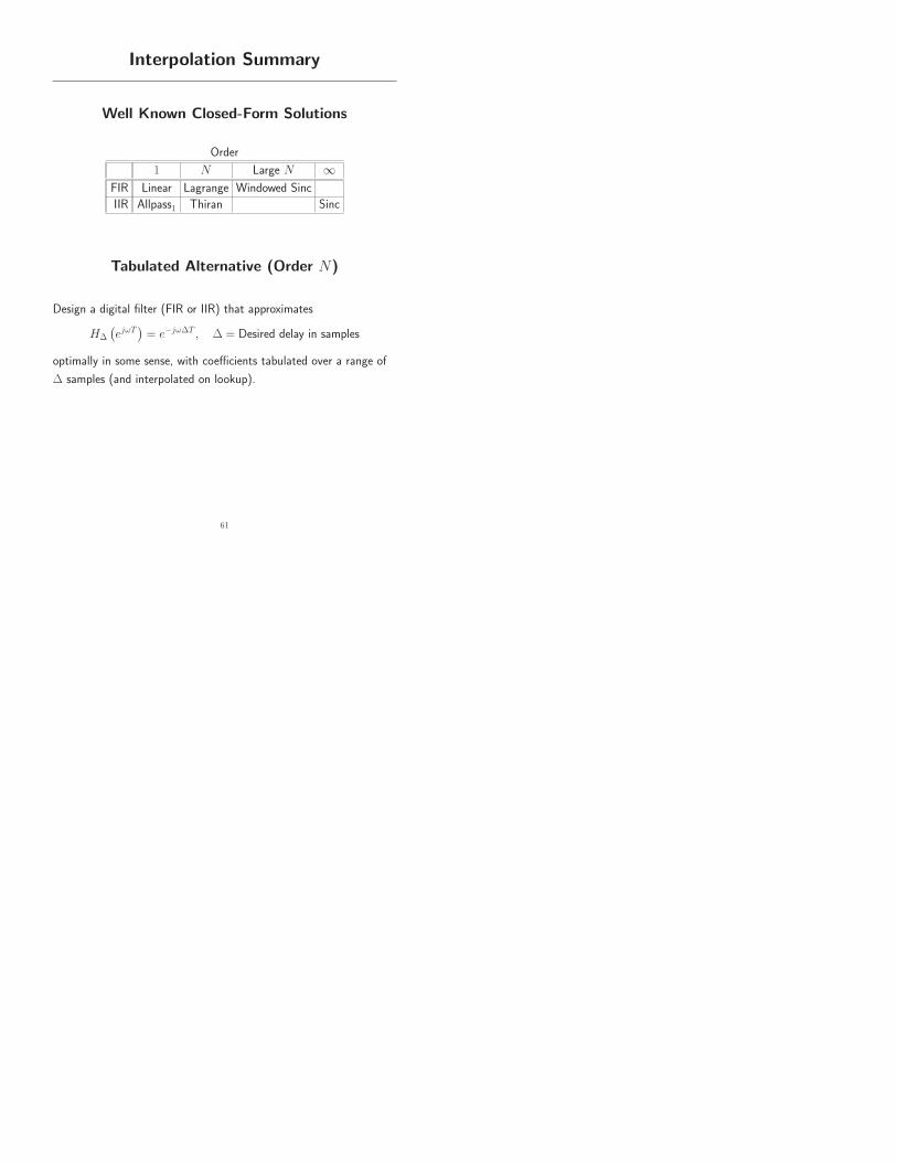
Interpolation Summary
Well Known Closed-Form Solutions
Order
1 N Large N ∞
FIR Linear Lagrange Windowed Sinc
IIR Allpass1 Thiran Sinc
Tabulated Alternative (Order N)
Design a digital filter (FIR or IIR) that approximates
H∆
(
ejωT)
= e−jω∆T , ∆ = Desired delay in samples
optimally in some sense, with coefficients tabulated over a range of
∆ samples (and interpolated on lookup).
61