A Probability Review

Outline:

A probability review.

Shorthand notation: RV stands for random variable.

EE 527, Detection and Estimation Theory, # 0b 1

A Probability Review

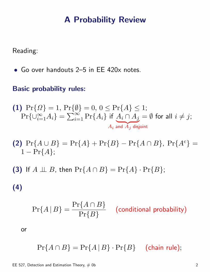
Reading:

Go over handouts 25 in EE 420x notes.

Basic probability rules:

(1) Pr{} = 1, Pr{} = 0, 0 Pr{A} 1;Pr{i=1Ai} =

i=1 Pr{Ai} if Ai Aj

Ai and Aj disjoint

= for all i 6= j;

(2) Pr{A B} = Pr{A} + Pr{B} Pr{A B}, Pr{Ac} =1 Pr{A};

(3) If A B, then Pr{A B} = Pr{A} Pr{B};

(4)

Pr{A |B} = Pr{A B}Pr{B}

(conditional probability)

or

Pr{A B} = Pr{A |B} Pr{B} (chain rule);

EE 527, Detection and Estimation Theory, # 0b 2

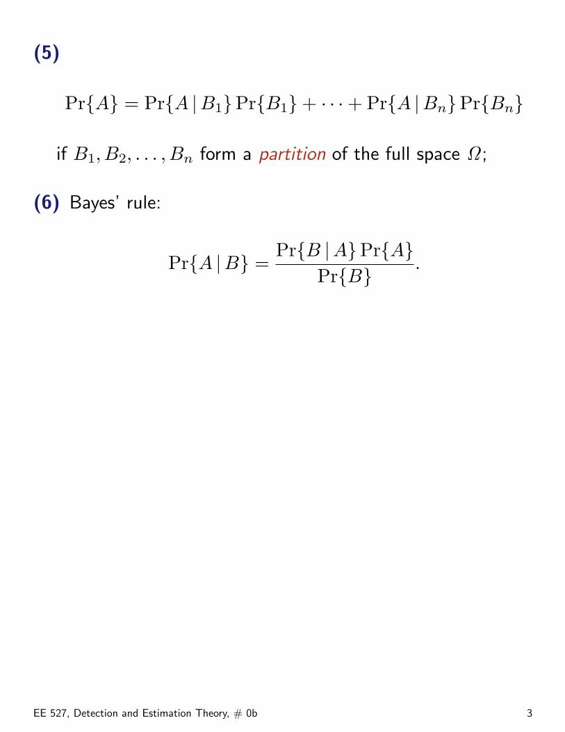
(5)

Pr{A} = Pr{A |B1}Pr{B1}+ + Pr{A |Bn}Pr{Bn}

if B1, B2, . . . , Bn form a partition of the full space ;

(6) Bayes rule:

Pr{A |B} = Pr{B |A}Pr{A}Pr{B}

.

EE 527, Detection and Estimation Theory, # 0b 3

Reminder: Independence, Correlation andCovariance

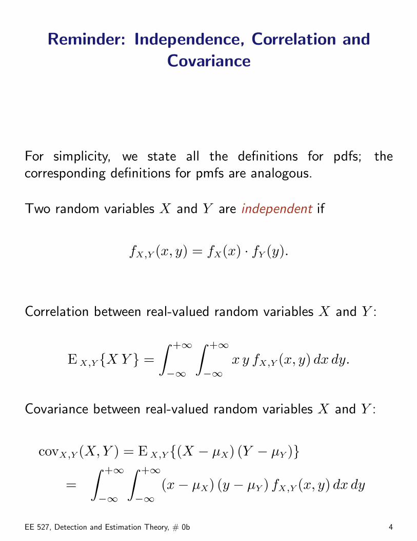
For simplicity, we state all the definitions for pdfs; thecorresponding definitions for pmfs are analogous.

Two random variables X and Y are independent if

fX,Y (x, y) = fX(x) fY (y).

Correlation between real-valued random variables X and Y :

E X,Y {X Y } = +

+

x y fX,Y (x, y) dx dy.

Covariance between real-valued random variables X and Y :

covX,Y (X, Y ) = E X,Y {(X X) (Y Y )}

= +

+

(x X) (y Y ) fX,Y (x, y) dx dy

EE 527, Detection and Estimation Theory, # 0b 4

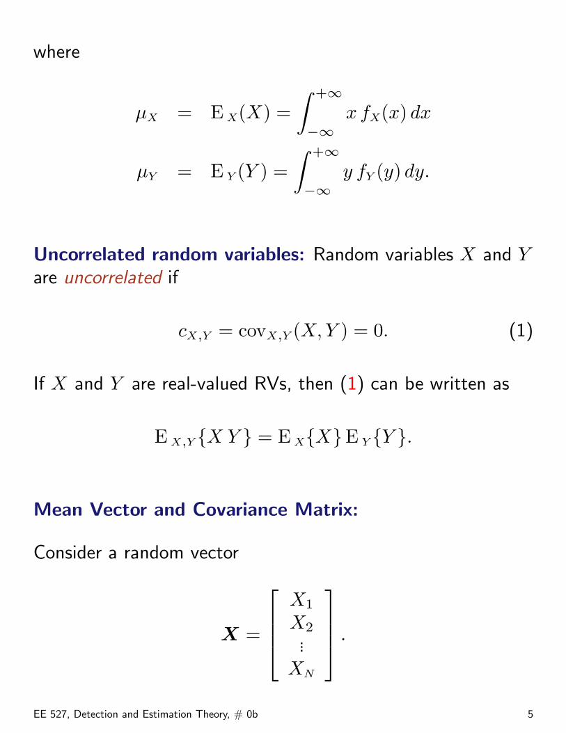
where

X = E X(X) = +

x fX(x) dx

Y = E Y (Y ) = +

y fY (y) dy.

Uncorrelated random variables: Random variables X and Yare uncorrelated if

cX,Y = covX,Y (X, Y ) = 0. (1)

If X and Y are real-valued RVs, then (1) can be written as

E X,Y {X Y } = E X{X}E Y {Y }.

Mean Vector and Covariance Matrix:

Consider a random vector

X =

X1X2...

XN

.EE 527, Detection and Estimation Theory, # 0b 5

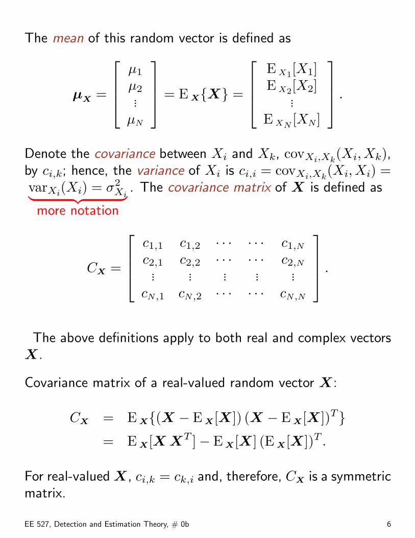
The mean of this random vector is defined as

X =

12...

N

= E X{X} =

E X1[X1]E X2[X2]

...E XN [XN ]

.Denote the covariance between Xi and Xk, covXi,Xk(Xi, Xk),by ci,k; hence, the variance of Xi is ci,i = covXi,Xk(Xi, Xi) =varXi(Xi) =

2Xi

more notation

. The covariance matrix of X is defined as

CX =

c1,1 c1,2 c1,Nc2,1 c2,2 c2,N... ... ... ... ...

cN,1 cN,2 cN,N

.

The above definitions apply to both real and complex vectorsX.

Covariance matrix of a real-valued random vector X:

CX = E X{(X E X[X]) (X E X[X])T}= E X[X XT ] E X[X] (E X[X])T .

For real-valued X, ci,k = ck,i and, therefore, CX is a symmetricmatrix.

EE 527, Detection and Estimation Theory, # 0b 6

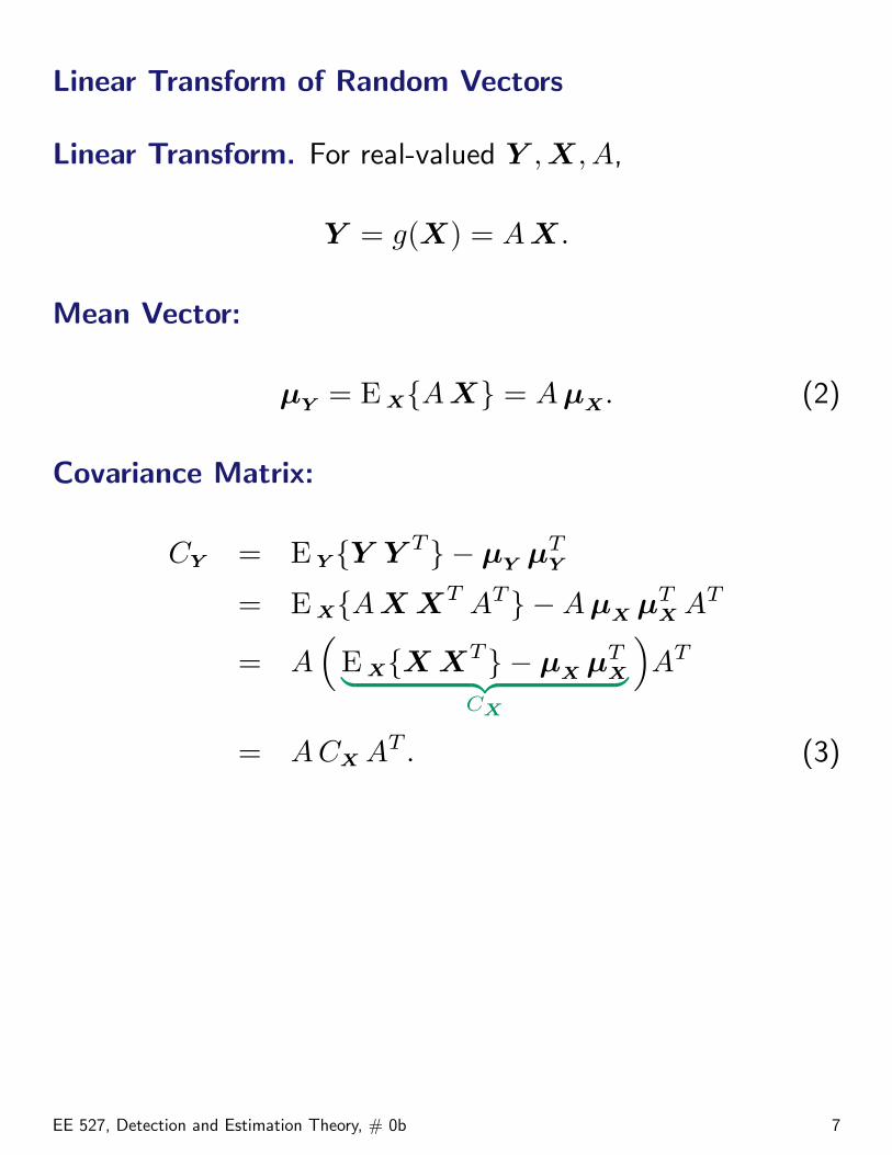
Linear Transform of Random Vectors

Linear Transform. For real-valued Y ,X, A,

Y = g(X) = A X.

Mean Vector:

Y = E X{A X} = A X. (2)

Covariance Matrix:

CY = E Y {Y Y T} Y TY= E X{A X XT AT} A X TX AT

= A(

E X{X XT} X TX CX

)AT

= A CX AT . (3)

EE 527, Detection and Estimation Theory, # 0b 7

Reminder: Iterated Expectations

In general, we can find E X,Y [g(X, Y )] using iteratedexpectations:

E X,Y [g(X, Y )] = E Y {E X | Y [g(X, Y ) |Y ]} (4)

where E X | Y denotes the expectation with respect to fX|Y (x | y)and E Y denotes the expectation with respect to fY (y).

Proof.

E Y {E X | Y [g(X, Y ) |Y ]} = +

E X | Y [g(X, Y ) | y] fY (y) dy

= +

( +

g(x, y)fX | Y (x | y) dx)fY (y) dy

= +

+

g(x, y)fX | Y (x | y)fY (y) dx dy

= +

+

g(x, y) fX,Y (x, y) dx dy

= E X,Y [g(X, Y )].

2

EE 527, Detection and Estimation Theory, # 0b 8

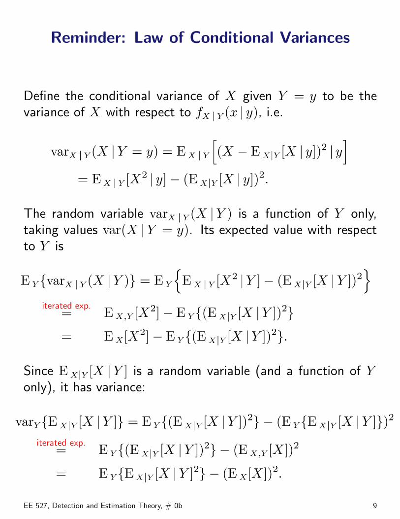
Reminder: Law of Conditional Variances

Define the conditional variance of X given Y = y to be thevariance of X with respect to fX | Y (x | y), i.e.

varX | Y (X |Y = y) = E X | Y[(X E X|Y [X | y])2 | y

]= E X | Y [X2 | y] (E X|Y [X | y])2.

The random variable varX | Y (X |Y ) is a function of Y only,taking values var(X |Y = y). Its expected value with respectto Y is

E Y {varX | Y (X |Y )} = E Y{

E X | Y [X2 |Y ] (E X|Y [X |Y ])2}

iterated exp.= E X,Y [X2] E Y {(E X|Y [X |Y ])2}

= E X[X2] E Y {(E X|Y [X |Y ])2}.

Since E X|Y [X |Y ] is a random variable (and a function of Yonly), it has variance:

varY {E X|Y [X |Y ]} = E Y {(E X|Y [X |Y ])2} (E Y {E X|Y [X |Y ]})2

iterated exp.= E Y {(E X|Y [X |Y ])2} (E X,Y [X])2

= E Y {E X|Y [X |Y ]2} (E X[X])2.

EE 527, Detection and Estimation Theory, # 0b 9

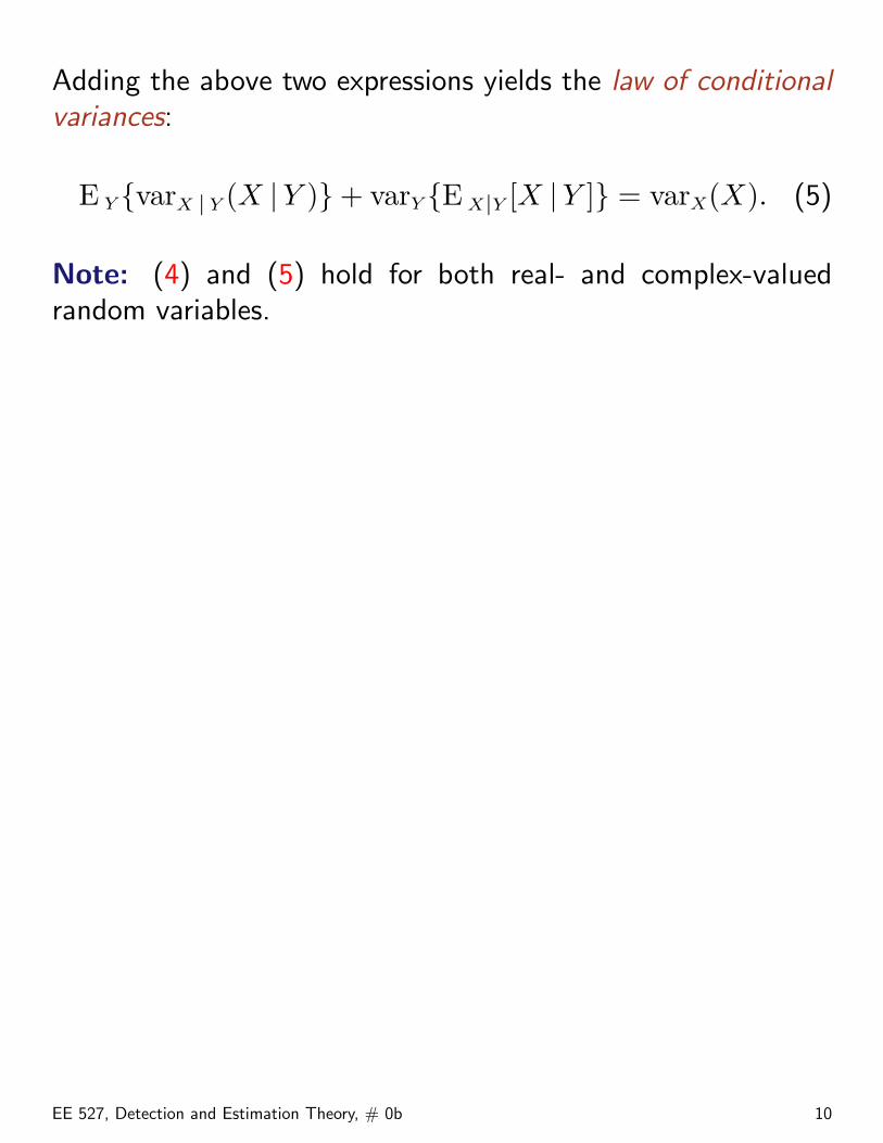
Adding the above two expressions yields the law of conditionalvariances:

E Y {varX | Y (X |Y )}+ varY {E X|Y [X |Y ]} = varX(X). (5)

Note: (4) and (5) hold for both real- and complex-valuedrandom variables.

EE 527, Detection and Estimation Theory, # 0b 10

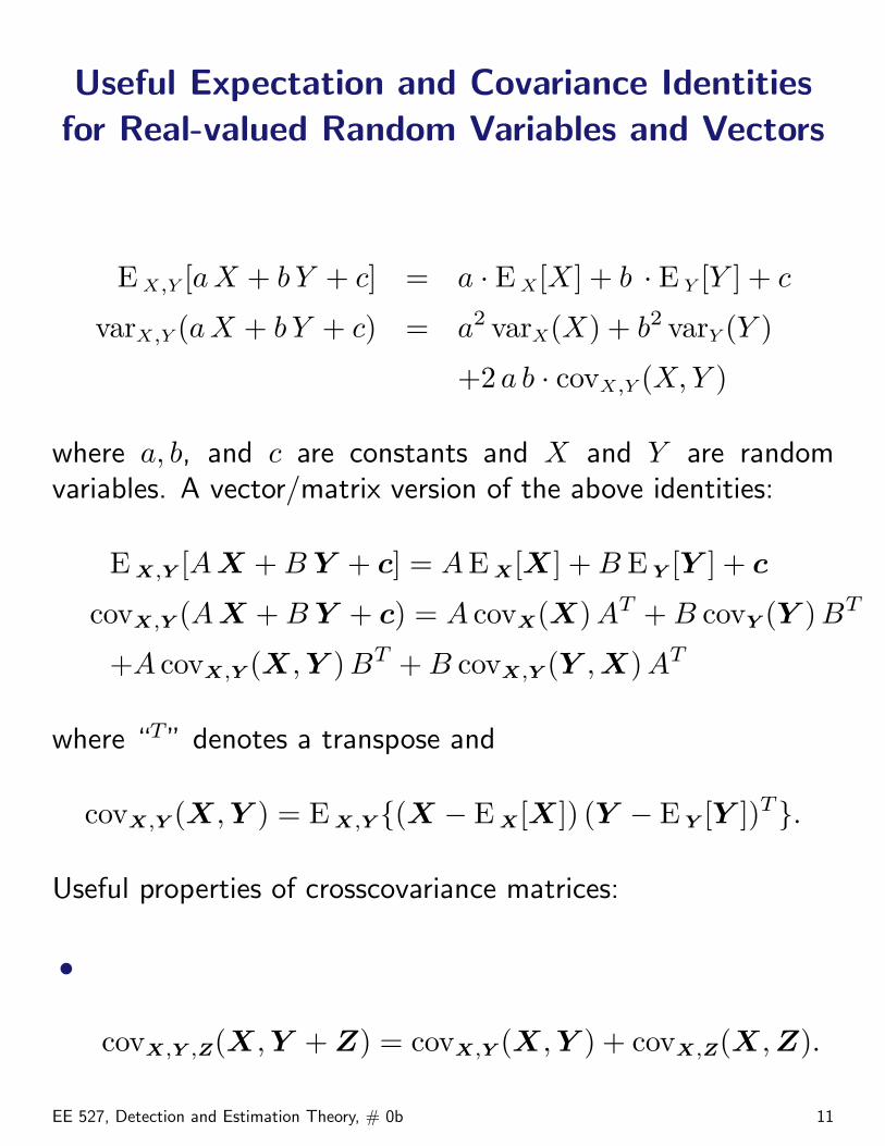
Useful Expectation and Covariance Identitiesfor Real-valued Random Variables and Vectors

E X,Y [aX + b Y + c] = a E X[X] + b E Y [Y ] + cvarX,Y (aX + b Y + c) = a2 varX(X) + b2 varY (Y )

+2 a b covX,Y (X, Y )

where a, b, and c are constants and X and Y are randomvariables. A vector/matrix version of the above identities:

E X,Y [A X + B Y + c] = A E X[X] + B E Y [Y ] + c

covX,Y (A X + B Y + c) = A covX(X) AT + B covY (Y ) BT

+A covX,Y (X,Y ) BT + B covX,Y (Y ,X) AT

where T denotes a transpose and

covX,Y (X,Y ) = E X,Y {(X E X[X]) (Y E Y [Y ])T}.

Useful properties of crosscovariance matrices:

covX,Y ,Z(X,Y + Z) = covX,Y (X,Y ) + covX,Z(X,Z).

EE 527, Detection and Estimation Theory, # 0b 11

covY ,X(Y ,X) = [covX,Y (X,Y )]T .

covX(X) = covX(X,X)

varX(X) = covX(X, X).

covX,Y (A X + b, P Y + q) = A covX,Y (X,Y ) PT .

(To refresh memory about covariance and its properties, see p.12 of handout 5 in EE 420x notes. For random vectors, seehandout 7 in EE 420x notes, particularly pp. 115.)

Useful theorems:

(1) (handout 5 in EE 420x notes)

E X(X) = E Y [E X | Y (X |Y )] shown on p. 8E X | Y [g(X) h(Y ) | y] = h(y) E X | Y [g(X) | y]E X,Y [g(X) h(Y )] = E Y {h(Y ) E X | Y [g(X) |Y ]}.

The vector version of (1) is the same just put bold letters.

EE 527, Detection and Estimation Theory, # 0b 12

(2)

varX(X) = E Y [varX | Y (X |Y )] + varY (E X | Y [X|Y ]);

and the vector/matrix version is

covX(X) variance/covariance

matrix of X

= E Y [covX | Y (X |Y )]

+covY (E X | Y [X|Y ]) shown on p. .

(3) Generalized law of conditional variances:

covX,Y (X, Y ) = E Z[covX,Y | Z(X, Y |Z)]+covZ(E X | Z[X |Z],E Y | Z[Y |Z]).

(4) Transformation:

Y = g(X) one-to-oneY1 = g1(X1, . . . , Xn)

...Yn = gn(X1, . . . , Xn)

thenfY (y) = fX(h1(y1), . . . , hn(yn)) |J |

EE 527, Detection and Estimation Theory, # 0b 13

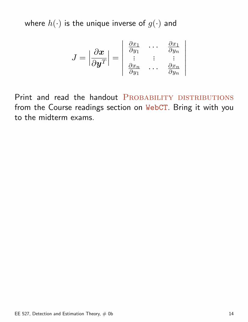
where h() is the unique inverse of g() and

J = xyT

=

x1y1

x1yn... ... ...xny1

xnyn

Print and read the handout Probability distributionsfrom the Course readings section on WebCT. Bring it with youto the midterm exams.

EE 527, Detection and Estimation Theory, # 0b 14

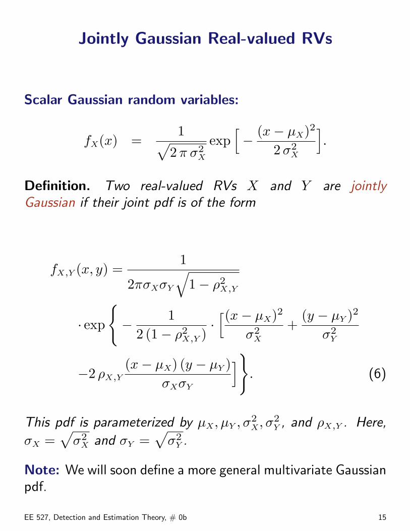
Jointly Gaussian Real-valued RVs

Scalar Gaussian random variables:

fX(x) =1

2 2Xexp

[ (x X)

2

2 2X

].

Definition. Two real-valued RVs X and Y are jointlyGaussian if their joint pdf is of the form

fX,Y (x, y) =1

2XY

1 2X,Y

exp

{ 1

2 (1 2X,Y )[(x X)2

2X+

(y Y )2

2Y

2 X,Y(x X) (y Y )

XY

]}. (6)

This pdf is parameterized by X, Y , 2X,

2Y , and X,Y . Here,

X =

2X and Y =

2Y .

Note: We will soon define a more general multivariate Gaussianpdf.

EE 527, Detection and Estimation Theory, # 0b 15

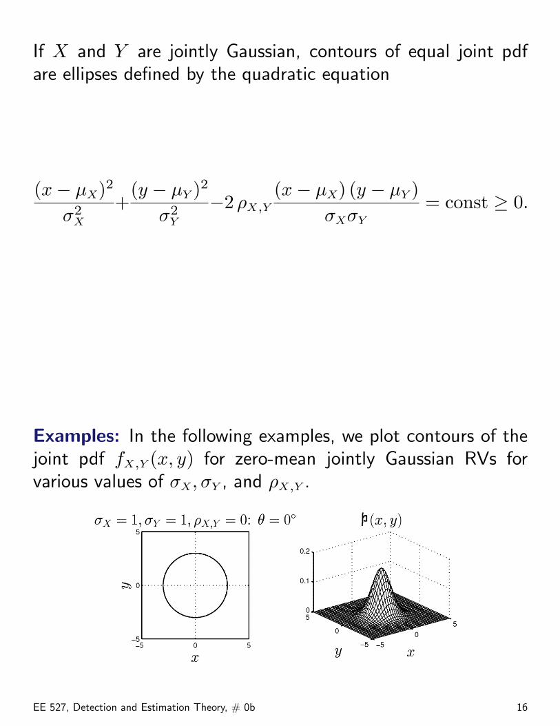
If X and Y are jointly Gaussian, contours of equal joint pdfare ellipses defined by the quadratic equation

(x X)2

2X+

(y Y )2

2Y2 X,Y

(x X) (y Y )XY

= const 0.

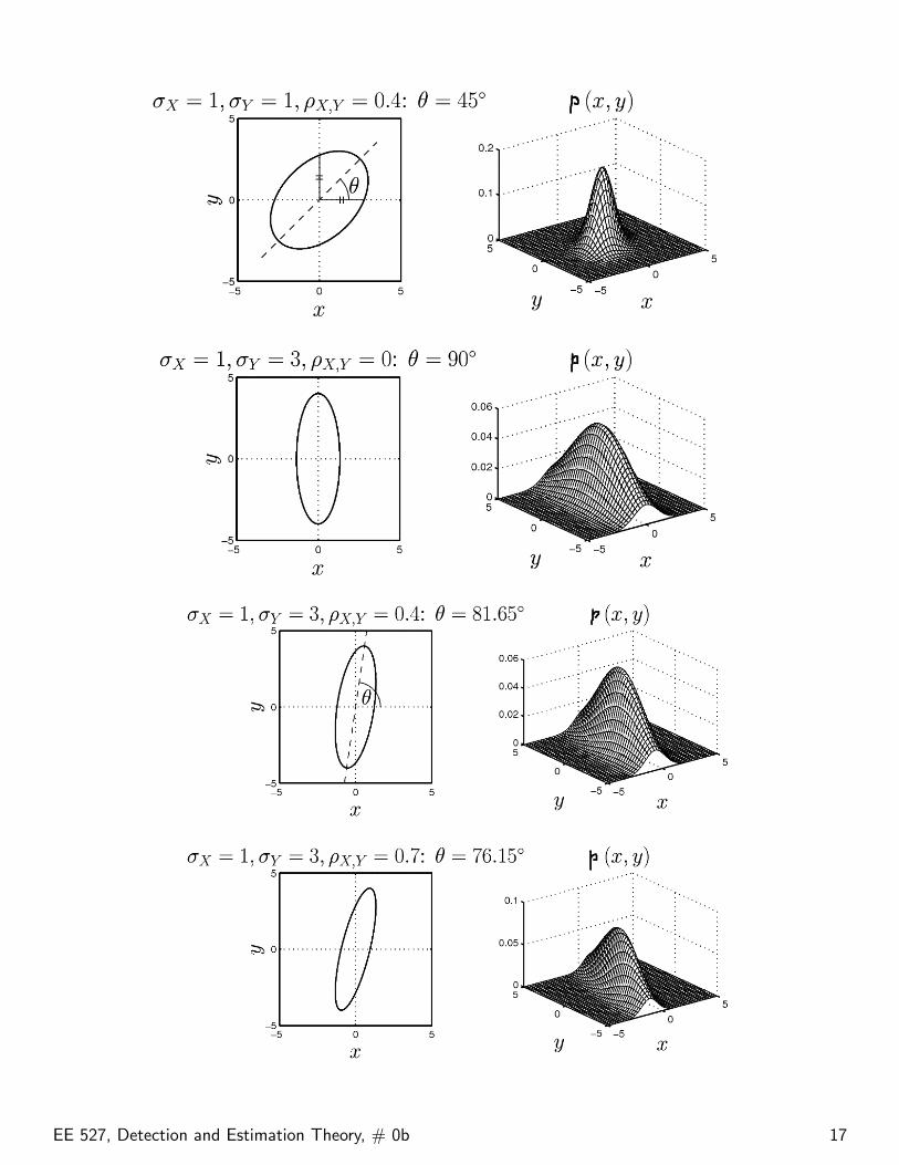
Examples: In the following examples, we plot contours of thejoint pdf fX,Y (x, y) for zero-mean jointly Gaussian RVs forvarious values of X, Y , and X,Y .

EE 527, Detection and Estimation Theory, # 0b 16

EE 527, Detection and Estimation Theory, # 0b 17

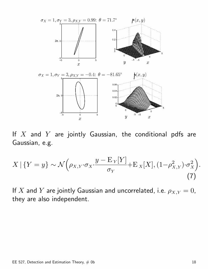
If X and Y are jointly Gaussian, the conditional pdfs areGaussian, e.g.

X | {Y = y} N(X,Y X

y E Y [Y ]Y

+E X[X], (12X,Y )2X).

(7)

If X and Y are jointly Gaussian and uncorrelated, i.e. X,Y = 0,they are also independent.

EE 527, Detection and Estimation Theory, # 0b 18

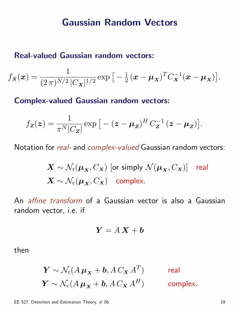
Gaussian Random Vectors

Real-valued Gaussian random vectors:

fX(x) =1

(2 )N/2 |CX|1/2exp

[ 12 (x X)

TC1X (x X)].

Complex-valued Gaussian random vectors:

fZ(z) =1

N |CZ|exp

[ (z Z)H C1Z (z Z)

].

Notation for real- and complex-valued Gaussian random vectors:

X Nr(X, CX) [or simply N (X, CX)] realX Nc(X, CX) complex.

An affine transform of a Gaussian vector is also a Gaussianrandom vector, i.e. if

Y = A X + b

then

Y Nr(A X + b, A CX AT ) realY Nc(A X + b, A CX AH) complex.

EE 527, Detection and Estimation Theory, # 0b 19

The Gaussian random vector W Nr(0, 2 In) (where Indenotes the identity matrix of size n) is called white; pdfcontours of a white Gaussian random vector are spherescentered at the origin. Suppose that W [n], n = 0, 1, . . . , N 1 are independent, identically distributed (i.i.d.) zero-mean univariate Gaussian N (0, 2). Then, for W =[W [0],W [1], . . . ,W [N 1]]T ,

fW (w) = N (w |0, 2 I).

Suppose now that, for these W [n],

Y [n] = + W [n]

where is a constant. What is the joint pdf of Y [0], Y [1], . . .,and Y [N 1]? This pdf is the pdf of the vector Y =[Y [0], Y [1], . . . , Y [N 1]]T :

Y = 1 + W

where 1 is an N 1 vector of ones. Now,

fY (y) = N (y |1 , 2 I).

Since is a constant,

fY (y) = fY | (y | ).

EE 527, Detection and Estimation Theory, # 0b 20

Gaussian Random Vectors

A real-valued random vector X = [X1, X2, . . . , Xn]T with

mean and covariance matrix with determinant | | > 0 (i.e. is

positive definite)

is a Gaussian random vector (or X1, X2, . . . , Xn are jointlyGaussian RVs) if and only if its joint pdf is

fX(x) =1

|2 |1/2exp[12 (x )

T1(x )]. (8)

Verify that, for n = 2, this joint pdf reduces to the two-dimensional pdf in (6).

Notation: We use X N (, ) to denote a Gaussian randomvector. Since is positive definite, 1 is also positive definiteand, for x 6= ,

(x )T1(x ) > 0

which means that the contours of the multivariate Gaussianpdf in (8) are ellipsoids.

The Gaussian random vector X N (0, 2In) (where Indenotes the identity matrix of size n) is called white contours of the pdf of a white Gaussian random vector arespheres centered at the origin.

EE 527, Detection and Estimation Theory, # 0b 21

Properties of Real-valued Gaussian RandomVectors

Property 1: For a Gaussian random vector, uncorrelationimplies independence.

This is easy to verify by setting i,j = 0 for all i 6= j inthe joint pdf, then becomes diagonal and so does 1;then, the joint pdf reduces to the product of marginal pdfsfXi(xi) = N (i,i,i) = N (i, 2Xi). Clearly, this propertyholds for blocks of RVs (subvectors) as well.

Property 2: A linear transform of a Gaussian random vectorX N (X,X) yields a Gaussian random vector:

Y = A X N (A X, AX AT ).

It is easy to show that E Y [Y ] = A X and covY (Y ) = Y =AX AT . So

E Y [Y ] = E X[A X] = A E X[X] = A X

and

Y = E Y [(Y E Y [Y ]) (Y E Y [Y ])T ]= E X[(A X A X) (A X A X)T ]= A E X[(X X) (X X)T ]AT = AX AT .

EE 527, Detection and Estimation Theory, # 0b 22

Of course, if we use the definition of a Gaussian random vectorin (8), we cannot yet claim that Y is a Gaussian randomvector. (For a different definition of a Gaussian random vector,we would be done right here.)

Proof. We need to verify that the joint pdf of Y indeed hasthe right form. Here, we decide to take the equivalent (easier)task and verify that the characteristic function of Y has theright form.

Definition. Suppose X fX(X). Then the characteristicfunction of X is given by

X() = E X[exp(j T X)]

where is an n-dimensional real-valued vector and j =1.

Thus

X() = +

+

fX(x) exp(j T x) dx

proportional to the inverse multi-dimensional Fourier transformof fX(x); therefore, we can find fX(x) by taking the Fouriertransform (with the appropriate proportionality factor):

fX(x) =1

(2)n

+

+

X() exp(j T x) dx

EE 527, Detection and Estimation Theory, # 0b 23

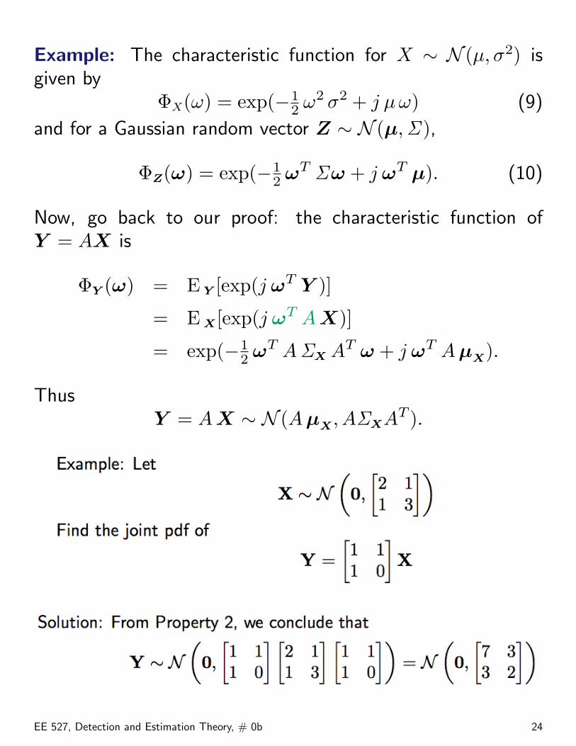
Example: The characteristic function for X N (, 2) isgiven by

X() = exp(12 2 2 + j ) (9)

and for a Gaussian random vector Z N (, ),

Z() = exp(12 T + j T ). (10)

Now, go back to our proof: the characteristic function ofY = AX is

Y () = E Y [exp(j T Y )]

= E X[exp(j T A X)]

= exp(12 T AX AT + j T A X).

ThusY = A X N (A X, AXAT ).

EE 527, Detection and Estimation Theory, # 0b 24

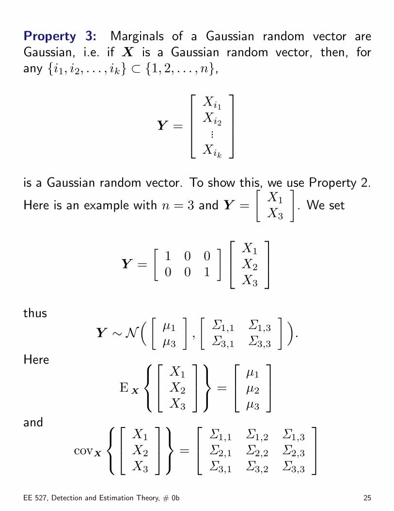
Property 3: Marginals of a Gaussian random vector areGaussian, i.e. if X is a Gaussian random vector, then, forany {i1, i2, . . . , ik} {1, 2, . . . , n},

Y =

Xi1Xi2...

Xik

is a Gaussian random vector. To show this, we use Property 2.

Here is an example with n = 3 and Y =[

X1X3

]. We set

Y =[

1 0 00 0 1

] X1X2X3

thus

Y N( [

13

],

[1,1 1,33,1 3,3

]).

Here

E X

X1X2

X3

= 12

3

and

covX

X1X2

X3

= 1,1 1,2 1,32,1 2,2 2,3

3,1 3,2 3,3

EE 527, Detection and Estimation Theory, # 0b 25

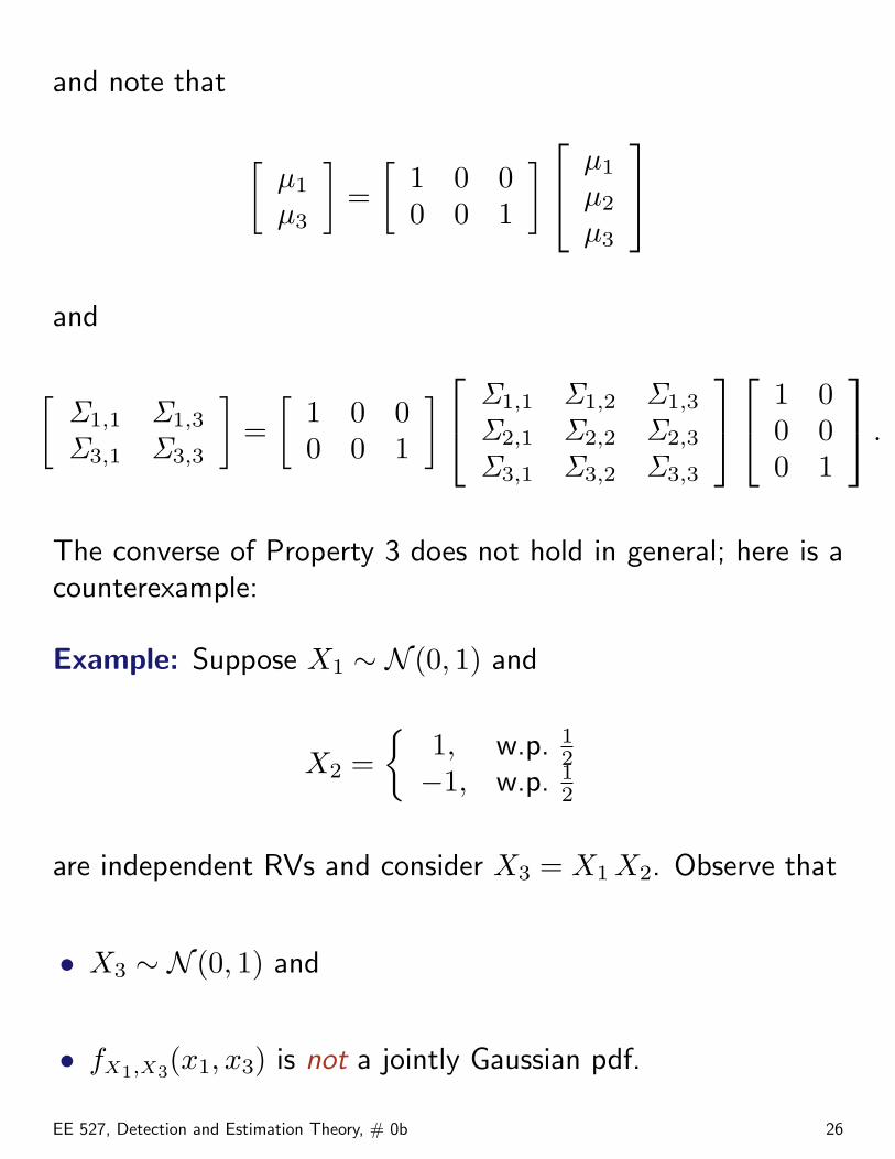
and note that

[13

]=

[1 0 00 0 1

] 123

and

[1,1 1,33,1 3,3

]=

[1 0 00 0 1

] 1,1 1,2 1,32,1 2,2 2,33,1 3,2 3,3

1 00 00 1

.The converse of Property 3 does not hold in general; here is acounterexample:

Example: Suppose X1 N (0, 1) and

X2 ={

1, w.p. 121, w.p. 12

are independent RVs and consider X3 = X1 X2. Observe that

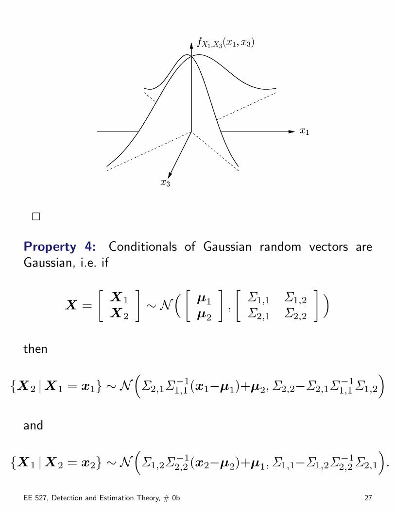
X3 N (0, 1) and

fX1,X3(x1, x3) is not a jointly Gaussian pdf.

EE 527, Detection and Estimation Theory, # 0b 26

2

Property 4: Conditionals of Gaussian random vectors areGaussian, i.e. if

X =[

X1X2

] N

( [12

],

[1,1 1,22,1 2,2

])then

{X2 |X1 = x1} N(2,111,1 (x11)+2,2,22,1

11,11,2

)and

{X1 |X2 = x2} N(1,212,2 (x22)+1,1,11,2

12,22,1

).

EE 527, Detection and Estimation Theory, # 0b 27

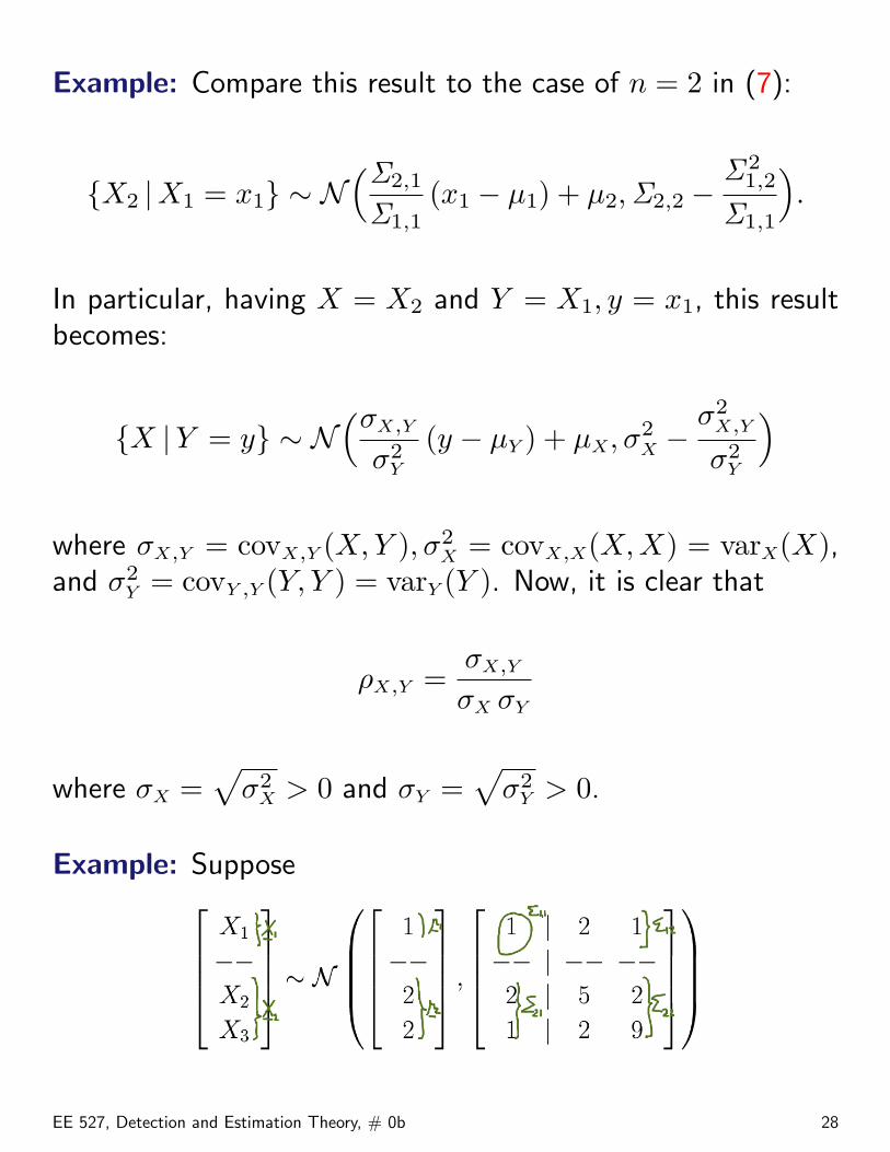
Example: Compare this result to the case of n = 2 in (7):

{X2 |X1 = x1} N(2,11,1

(x1 1) + 2,2,2 21,21,1

).

In particular, having X = X2 and Y = X1, y = x1, this resultbecomes:

{X |Y = y} N(X,Y

2Y(y Y ) + X, 2X

2X,Y2Y

)

where X,Y = covX,Y (X, Y ), 2X = covX,X(X, X) = varX(X),and 2Y = covY ,Y (Y, Y ) = varY (Y ). Now, it is clear that

X,Y =X,YX Y

where X =

2X > 0 and Y =

2Y > 0.

Example: Suppose

EE 527, Detection and Estimation Theory, # 0b 28

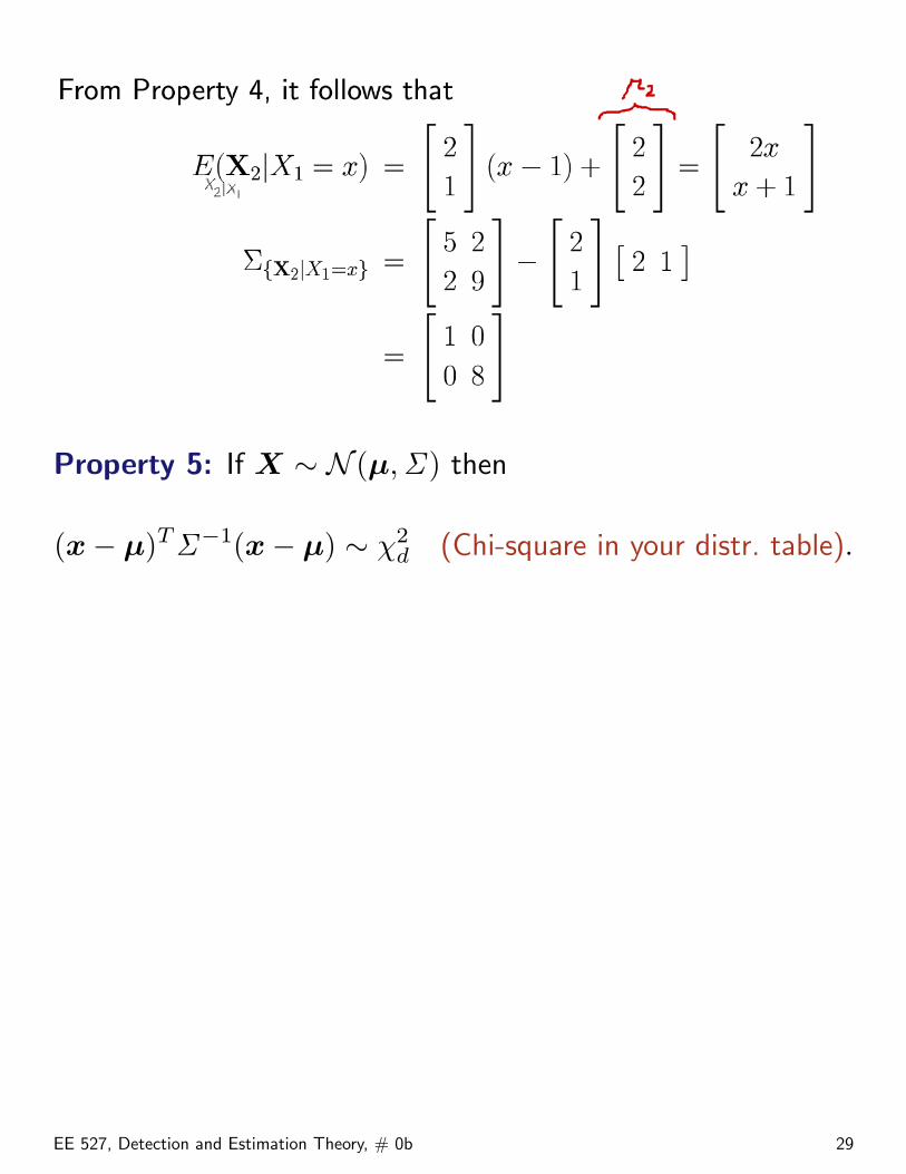
Property 5: If X N (, ) then

(x )T1(x ) 2d (Chi-square in your distr. table).

EE 527, Detection and Estimation Theory, # 0b 29

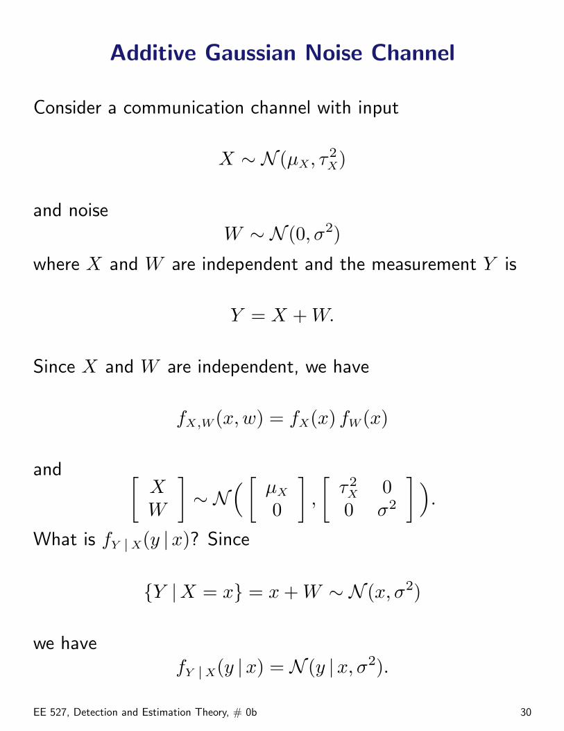
Additive Gaussian Noise Channel

Consider a communication channel with input

X N (X, 2X)

and noiseW N (0, 2)

where X and W are independent and the measurement Y is

Y = X + W.

Since X and W are independent, we have

fX,W(x,w) = fX(x) fW(x)

and [XW

] N

( [X0

],

[2X 00 2

]).

What is fY |X(y |x)? Since

{Y |X = x} = x + W N (x, 2)

we havefY |X(y |x) = N (y |x, 2).

EE 527, Detection and Estimation Theory, # 0b 30

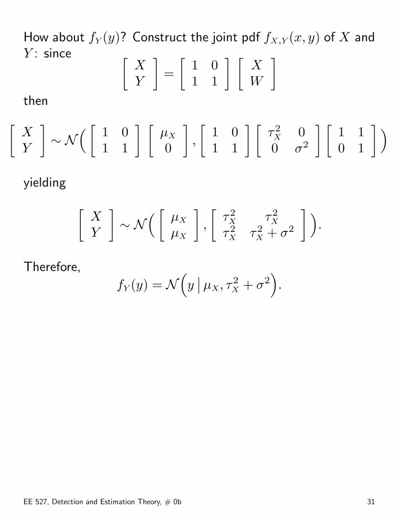
How about fY (y)? Construct the joint pdf fX,Y (x, y) of X andY : since [

XY

]=

[1 01 1

] [XW

]then[XY

] N

( [ 1 01 1

] [X0

],

[1 01 1

] [2X 00 2

] [1 10 1

])yielding [

XY

] N

( [XX

],

[2X

2X

2X 2X +

2

]).

Therefore,

fY (y) = N(y

X, 2X + 2).

EE 527, Detection and Estimation Theory, # 0b 31

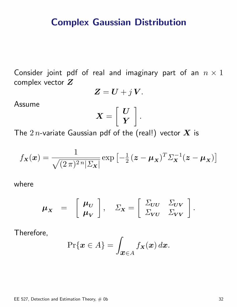
Complex Gaussian Distribution

Consider joint pdf of real and imaginary part of an n 1complex vector Z

Z = U + j V .

Assume

X =[

UY

].

The 2 n-variate Gaussian pdf of the (real!) vector X is

fX(x) =1

(2 )2 n|X|exp

[12 (z X)

T1X (z X)]

where

X =[

UV

], X =

[UU UVV U V V

].

Therefore,

Pr{x A} =xA

fX(x) dx.

EE 527, Detection and Estimation Theory, # 0b 32

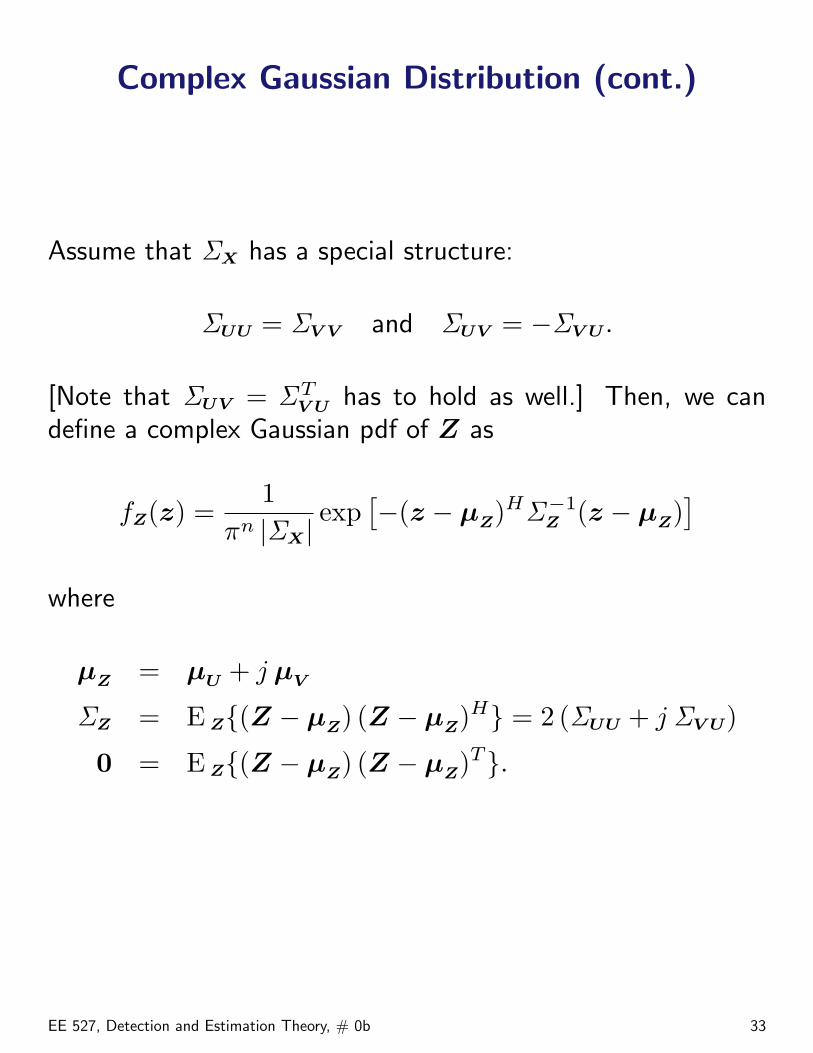
Complex Gaussian Distribution (cont.)

Assume that X has a special structure:

UU = V V and UV = V U .

[Note that UV = TV U has to hold as well.] Then, we candefine a complex Gaussian pdf of Z as

fZ(z) =1

n |X|exp

[(z Z)H1Z (z Z)

]where

Z = U + j VZ = E Z{(Z Z) (Z Z)H} = 2 (UU + j V U)0 = E Z{(Z Z) (Z Z)T}.

EE 527, Detection and Estimation Theory, # 0b 33