Oscillating particles in fluids: Theory, experiment and ... · Landau and Lifshitz, "Physical...
87
Oscillating particles in fluids: Theory, experiment and numerics Oscillating particles in fluids: Theory, experiment and numerics Victor Yakhot Boston University, Boston, MA May, 2012, Vienna
Transcript of Oscillating particles in fluids: Theory, experiment and ... · Landau and Lifshitz, "Physical...
Oscillating particles in fluids: Theory, experiment and numerics
Oscillating particles in fluids: Theory, experimentand numerics
Victor YakhotBoston University, Boston, MA
May, 2012, Vienna

Oscillating particles in fluids: Theory, experiment and numerics
Boltzmann-BGK Equation in the range 0 ≤ ωτ <∞
Experimental data. Universality.

Oscillating particles in fluids: Theory, experiment and numerics
My collaborators:
Kamil Ekinci (BU);Carlos Colosqui (BU→ Princeton);Devrez Karabacak (BU→Delft).
Hudong Chen, Xiaowen Shan, Ilya Staroselsky (EXA Corp.)

Oscillating particles in fluids: Theory, experiment and numerics
Landau and Lifshitz, ”Physical kinetics”. After presentingderivation of Boltzmann equation they mention in passing:
C ≈ − f − f eq
τ
with τ = const”... is a rough estimate of collision integral”This expression, which is at the foundation of BGK-LBM, hasnever been derived as a consistent approximation
Oscillating particles in fluids: Theory, experiment and numerics
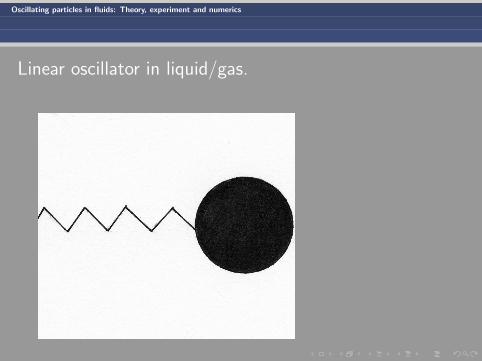
Linear oscillator in liquid/gas.

Oscillating particles in fluids: Theory, experiment and numerics
m0d2x
dt2+ γm0
dx
dt+ κx = R(t) (1)
d2x
dt2+ γ
dx
dt+ ω2
0x =R0
m0cosωt (2)
ω0 =√κ/m0
I (ω − ω0) =R20
8m0
γ
(ω − ω0)2 + γ2
4
The mass m0 = mR + mf where mR is the resonator mass invacuum and the added mass mf is that of the fluid ‘pushed’ by theresonator.The damping γ = γR + γf where γf is FLUIDIC DISSIPATION
Oscillating particles in fluids: Theory, experiment and numerics
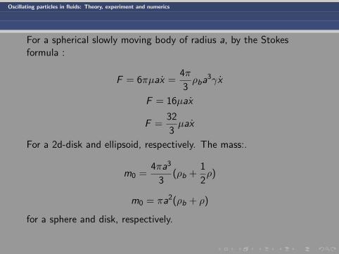
For a spherical slowly moving body of radius a, by the Stokesformula :
F = 6πµax =4π
3ρba3γx
F = 16µax
F =32
3µax
For a 2d-disk and ellipsoid, respectively. The mass:.
m0 =4πa3
3(ρb +
1
2ρ)
m0 = πa2(ρb + ρ)
for a sphere and disk, respectively.
Oscillating particles in fluids: Theory, experiment and numerics
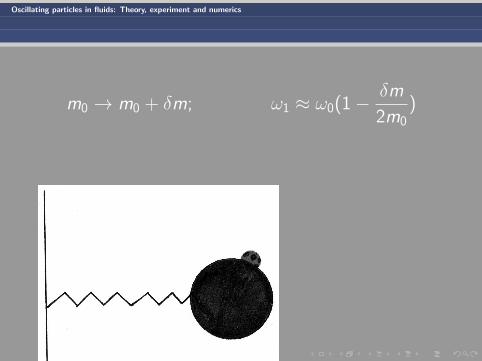
m0 → m0 + δm; ω1 ≈ ω0(1− δm
2m0)

Oscillating particles in fluids: Theory, experiment and numerics
Double-Clamped Beam. Schematic.
diagram.pdf
hw
lz(t)
!
~
hw
lz(t)
!
~
h ≈ 0.1µm, w ≈ 0.5µm, l ≈ 10µm .

Oscillating particles in fluids: Theory, experiment and numerics
Array of Nanobeams. Microscope. Dimensions → ω0

Oscillating particles in fluids: Theory, experiment and numerics
Nanobeams as Sensors.
FrequencyAm
plitu
de o
f Mot
ionBiomolecule
NEMS in Fluidic Enviroment

Oscillating particles in fluids: Theory, experiment and numerics
Nanobeams. Biodetection

Oscillating particles in fluids: Theory, experiment and numerics
Nanocantilevers. Biodetection
Oscillating particles in fluids: Theory, experiment and numerics
The modern devices:
m0 ≈ 10−13 − 10−12gr
ω0 ≈ 109Hz
One can work with higher harmonics and achieve higherfrequencies.
Now, detection of the mass of a proton is a reality.
Oscillating particles in fluids: Theory, experiment and numerics
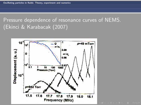
Pressure dependence of resonance curves of NEMS.(Ekinci & Karabacak (2007)

Oscillating particles in fluids: Theory, experiment and numerics
FDT.
(a)(b) (c)
.

Oscillating particles in fluids: Theory, experiment and numerics
FDT
.

Oscillating particles in fluids: Theory, experiment and numerics
In equilibrium if resonator is thermally excited, variance thedisplacement : ∫ ∞
−∞h2P(h)dh =
4kBT
κ
In a confined system this relation is not clear.
Experimental test of FDT
Oscillating particles in fluids: Theory, experiment and numerics
TO DETECT A MASS δm:
ω0δm
2m0 γ
THE MAIN STUMBLING BLOCK IN BIODETECTION ISFLUIDIC DISSIPATION IN WATER (FLUIDS).
FIRST WE HAVE TO UNDERSTAND IT.

Oscillating particles in fluids: Theory, experiment and numerics
This is not so simple. In air
p ≈ 800torr ; τmol−mol ≈ 0.2× 10⁻⁹sec
,
τmol−si ≈ 10−9sec
.
p = 100torr ; τmol−mol ≈ 10−9 − 10−8
.
0 ≤ ωτ ≤ 10− 100
Oscillating particles in fluids: Theory, experiment and numerics
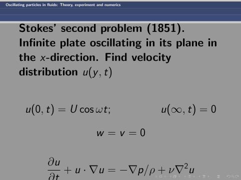
Stokes’ second problem (1851).Infinite plate oscillating in its plane inthe x-direction. Find velocitydistribution u(y , t)
u(0, t) = U cosωt; u(∞, t) = 0
w = v = 0
∂u
∂t+ u · ∇u = −∇p/ρ + ν∇2u

Oscillating particles in fluids: Theory, experiment and numerics
∂u
∂t= ν
∂2u
∂y 2
u(y , t) = Ue−yδ cos(ωt +
y
δ)
δ =
√2ν
ωOverdamped surface wave. No transverse
propagating shear waves. (Definition of fluid)

Oscillating particles in fluids: Theory, experiment and numerics
Force per unit area (viscous stress)
σ = ρν∂u
∂y|y=0 = −U
√ωρµ cos(ωt +
π
4)
Mean dissipation per unit time
−σu =U2
2
√ωµρ
2
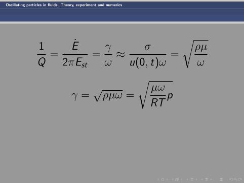
Quality factor Q
Oscillating particles in fluids: Theory, experiment and numerics
1
Q=
E
2πEst=γ
ω≈ σ
u(0, t)ω=
√ρµ
ω
γ =√ρµω =
√µω
RTp

Oscillating particles in fluids: Theory, experiment and numerics
Dissipation. x = ωτ
0 20 40 60 80 100x
0.51
510
delta
1 2 5 10 20 50 100x1
1.52
3
5
7
10gamma

Oscillating particles in fluids: Theory, experiment and numerics
Breakdown of Newtonian Hydrodynamics.
∂ui∂t
+ u·∇ui =1
ρ∇jρσij
σij = u′iu′j
Kinetic Theory. Boltzmann Equation.
σij = σ(1)ij + σ
(2)ij + ....
σ(1)ij ≈
ν
2(∂iuj + ∂jui) ≡ νSij

Oscillating particles in fluids: Theory, experiment and numerics
Different geometries. Different scales.
Oscillating particles in fluids: Theory, experiment and numerics
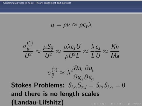
µ = ρν ≈ ρcsλ
σ(1)ij
U2≈ µSij
U2≈ ρλcsU
ρU2L≈ λ
L
csU≈ Kn
Ma
σ(2)ij ≈ λ2 ∂ui
∂xα
∂uj∂xα
Stokes Problems: Si ,αSα,j = SiαSj ,α = 0
and there is no length scales(Landau-Lifshitz)

Oscillating particles in fluids: Theory, experiment and numerics
σ(2)ij ≈ λ2Sij∇ · u
One has to solve dynamic kineticequation.

Oscillating particles in fluids: Theory, experiment and numerics
Stokes’ Second Problem, Revisited. KineticBoltzmann-BGK equation.
VY, Colosqui (2007).
∂f
∂t+ v · ∇f = −f − f eq
τ
f eq =ρ
(2πθ)32
exp(−(v −U(x, t))2
2θ)

Oscillating particles in fluids: Theory, experiment and numerics
Boltzmann’s collision integral:
C =
∫vrel(f ′f ′1 − ff1)dσdp1 ≈
− f
τ (f )+
∫vrel f
′f ′1dσdp1
τ (f ) =
∫vreldσf1dp1 ≈ τ = const???

Oscillating particles in fluids: Theory, experiment and numerics
Relaxation time τ ≈ const.
τ ≈ λ/v ≈ λ/cs
cs-speed of sound. In the air attemperature θ ≈ 300K and pressure
p = 1atm ≈ 1000torr
τ ≈ 200/p × 10−9sec ≈ 0.2× 10⁻⁹sec
At this point this relation does notaccount for solid walls, strong shear
etc.

Oscillating particles in fluids: Theory, experiment and numerics
∫C(f )dv =
∫C(f )vdv = 0
ρ =
∫f (v)dv
∂ρ
∂t+∇ · ρU(x) = 0
∂ρUj(x)
∂t+ ∂iρUj(x)Ui(x) + ∂iσij = 0

Oscillating particles in fluids: Theory, experiment and numerics
σij = ρ(vi − Ui(x))(vj − Uj(x))
The goal is to derive the expression forthe stress σij in terms of observables.
This can be done using theChapman-Enskog expansion.Hudong Chen et al (2004).

Oscillating particles in fluids: Theory, experiment and numerics
f = f (0) + εf (1) + ε2f (2) + · · ·
∂t = ε∂t0 + ε2∂t1 + · · ·∇ = ε∇1

Oscillating particles in fluids: Theory, experiment and numerics
In the zeroth order
f = f eq
σij |eq = ρθδij
(ideal gas):

Oscillating particles in fluids: Theory, experiment and numerics
f 1 = −τθ
f 0Sij [(vi − ui)(vj − uj)−(u− v)2
dδij
f (2) = −2τ 2f (0)[(vi−vj)∂j(Sij−∇·uδij .....)+++

Oscillating particles in fluids: Theory, experiment and numerics
∂Uj(x)
∂t+ Ui(x)∂iUj(x) +
1
ρ∇p(x) = 0
Oscillating particles in fluids: Theory, experiment and numerics
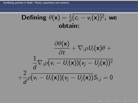
Defining θ(x) = 1d (ci − vi(x))2, we
obtain:
∂θ(x)
∂t+∇iρUi(x)θ +
1
d∇iρ(vi − Ui(x))(vj − Uj(x))2
+2
dρ(vi − Ui(x))(vj − Uj(x))Si ,j = 0

Oscillating particles in fluids: Theory, experiment and numerics
In the next order we derive Newtonianapproximation and NS Equations:
σ1 ≈ −2ρν(Sij −1
dδij∇ · u)
ν = θτ
Sij =1
2(∂ui∂xj
+∂uj∂ui
)

Oscillating particles in fluids: Theory, experiment and numerics
σ(2)ij = 2ρν ˙(τSij) +
4ρν2
θ(SikSkj − δijSklSkl/d)−
−2ρν2
θ(SikΩkj + SjkΩki)
A = (∂t + U · ∇)A
Ωij =1
2(U j
i − U ij )

Oscillating particles in fluids: Theory, experiment and numerics
σ(1)ij + σ
(2)ij = −2ρν(1− τ∂t)Sij
∂u
∂t+ u · ∇u = 2ρν(1− τ∂t)
∂2u
∂y 2
Oscillating particles in fluids: Theory, experiment and numerics
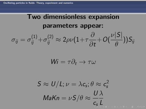
Two dimensionless expansionparameters appear:
σij = σ(1)ij +σ
(2)ij ≈ 2ρν(1+τ
∂
∂t+O(
ν|S |θ
))Sij
Wi = τ∂t → τω
S ≈ U/L; ν = λcs ; θ ≈ c2s
MaKn = νS/θ ≈ U
cs
λ
L
Oscillating particles in fluids: Theory, experiment and numerics
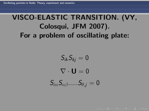
VISCO-ELASTIC TRANSITION. (VY,Colosqui, JFM 2007).
For a problem of oscillating plate:
SikSkj = 0
∇ ·U = 0
SiαSαβ.....Sθ,j = 0
Oscillating particles in fluids: Theory, experiment and numerics
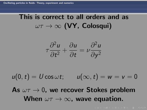
This is correct to all orders and asωτ →∞ (VY, Colosqui)
τ∂2u
∂t2+∂u
∂t= ν
∂2u
∂y 2
u(0, t) = U cosωt; u(∞, t) = w = v = 0
As ωτ → 0, we recover Stokes problemWhen ωτ →∞, wave equation.

Oscillating particles in fluids: Theory, experiment and numerics
All this can be exactly derived in anon-perturbative way (Chen,
Staroselsky, Orszag, Shan, VY...).
∂f
∂t+ v · ∇f = −f − f eq
τ
Interested in a unidirectional flow,which is incompressible, we, withoutloss of generality, set ρ = const = 1.
Oscillating particles in fluids: Theory, experiment and numerics
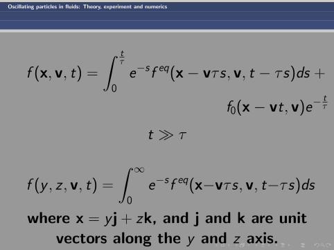
f (x, v, t) =
∫ tτ
0
e−sf eq(x− vτ s, v, t − τ s)ds +
f0(x− vt, v)e−tτ
t τ
f (y , z , v, t) =
∫ ∞0
e−sf eq(x−vτ s, v, t−τ s)ds
where x = y j + zk, and j and k are unitvectors along the y and z axis.

Oscillating particles in fluids: Theory, experiment and numerics
Spatial shift operator:F (x + a) = ea∂x F (x)
f (x, v, t) =
∫ ∞0
e−se−τsv·∇f eq(x, v, t−τ s)ds
Unidirectional flow: ρ = const = 1:
u(x, t) =
∫vdv
∫ ∞0
e−se−τsv·∇f eq(x, v, t−τ s)ds
(3)
Oscillating particles in fluids: Theory, experiment and numerics
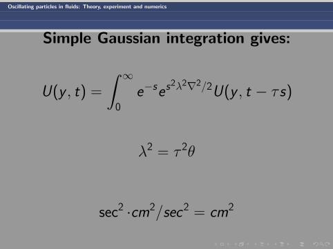
Simple Gaussian integration gives:
U(y , t) =
∫ ∞0
e−ses2λ2∇2/2U(y , t − τ s)
λ2 = τ 2θ
sec2 ·cm2/sec2 = cm2
Oscillating particles in fluids: Theory, experiment and numerics
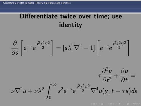
Differentiate twice over time; useidentity
∂
∂s
[e−se
s2λ2∇2
2
]= [sλ2∇2 − 1]
[e−se
s2λ2∇2
2
]
τ∂2u
∂t2+∂u
∂t=
ν∇2u + νλ2
∫ ∞0
s2e−ses2λ2∇2
2 ∇4u(y , t − τ s)ds

Oscillating particles in fluids: Theory, experiment and numerics
This hydrodynamic equation is exact.
τ∂2u
∂t2+∂u
∂t= ν(1 + φ)∇2u (4)
φ = λ2
∫ ∞0
dss2e−ses2λ2∇2
2 e−sτ∂t∇2 (5)
φ = −Wi
2
∫ ∞0
dss2e−s(1−iWi)− s2Wi2
2

Oscillating particles in fluids: Theory, experiment and numerics
Wi = ωτ → 0
ν = θτ ;∇2 ≈ 1/δ2 = ω/2ν =ω
2θτ
φ ≈ ωτ
2
∫ ∞0
dss2e−se−s2ωτ
4 e isωτ = ωτ → 0
∇2 = 1/δ2 = ω/2ν

Oscillating particles in fluids: Theory, experiment and numerics
Diffusion equation; Stokes’ problem;

Oscillating particles in fluids: Theory, experiment and numerics
Large-Weissenberg Limit Wi = ωτ 1:
φ ∼ −Wi
∫ 1√Wi
0
s2ds ∼ −Wi−1/2 → 0
∂2u
∂t2+
1
τ
∂u
∂t− c2∂
2u
∂y 2≡ Θu = 0 (6)
The TE derived from the CEexpansion before (VY, Colosqui. JFM
(2007).

Oscillating particles in fluids: Theory, experiment and numerics
Solution:
u = Ueyδ− cos(ωt − y
δ+)
δ
δ±=
(1 + ω2τ 2)14 [cos(
tan−1 ωτ
2)± sin(
tan−1 ωτ
2)]

Oscillating particles in fluids: Theory, experiment and numerics
We have three scales and three Knudsen
numbers:
δ; δ−; δ+
Kn =λ
δKn− =
λ
δ−; Kn+ =
λ
δ+
Oscillating particles in fluids: Theory, experiment and numerics
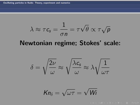
λ ≈ τcs =1
σn= τ√θ ∝ τ
√p
Newtonian regime; Stokes’ scale:
δ =
√2ν
ω≈√λcsω≈ λ
√1
ωτ
Knδ =√ωτ =
√Wi
Oscillating particles in fluids: Theory, experiment and numerics
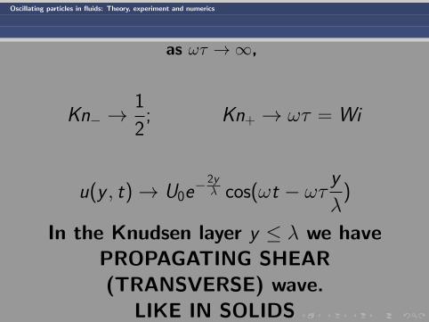
as ωτ →∞,
Kn− →1
2; Kn+ → ωτ = Wi
u(y , t)→ U0e−2yλ cos(ωt − ωτ y
λ)
In the Knudsen layer y ≤ λ we havePROPAGATING SHEAR(TRANSVERSE) wave.
LIKE IN SOLIDS

Oscillating particles in fluids: Theory, experiment and numerics
Boltzmann-BGK Equation in the range 0 ≤ ωτ <∞
Velocity distribution vs τω. Colosqui, VY. LBM-BGKequation.
widthwidth
Oscillating particles in fluids: Theory, experiment and numerics
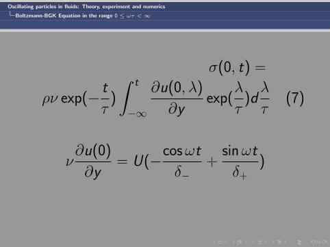
Boltzmann-BGK Equation in the range 0 ≤ ωτ <∞
σ(0, t) =
ρν exp(− t
τ)
∫ t
−∞
∂u(0, λ)
∂yexp(
λ
τ)dλ
τ(7)
ν∂u(0)
∂y= U(−cosωt
δ−+
sinωt
δ+)

Oscillating particles in fluids: Theory, experiment and numerics
Boltzmann-BGK Equation in the range 0 ≤ ωτ <∞
Ddissipation rate per unit time perunit area of the plate:
W = −u(0, t)σ(0, t)
W (τ, ω) =1
2
µU2
1 + ω2τ 2(
1
δ−+ωτ
δ+) (8)
(instead of√
p in Newtonian regime.

Oscillating particles in fluids: Theory, experiment and numerics
Boltzmann-BGK Equation in the range 0 ≤ ωτ <∞
Dissipation rate per cycle vs τω.
2 4 6 8 10
0.2
0.4
0.6
0.8
1
1.2
1.4

Oscillating particles in fluids: Theory, experiment and numerics
Experimental data. Universality.
Plane oscillator.
M∂ttx + Sγ∂tx + ω20x = MR(t)
∂ttx +γ
ρphp∂tx + ω2
0x = R(t)

Oscillating particles in fluids: Theory, experiment and numerics
Experimental data. Universality.
γxt = γu(0, t) = 2ρσ(0, t)/ms
ms = ρph
γ = gρ√ωpν
ρph(1 + ω2τ 2p )
34
×
[(1 + ωτp) cos(1
2tan−1ωτp)−
(1− ωτp) sin(1
2tan−1ωτp)]

Oscillating particles in fluids: Theory, experiment and numerics
Experimental data. Universality.
In general:
E ≡ W =SU2
2
√ωρµ
2f (ωτ )

Oscillating particles in fluids: Theory, experiment and numerics
Experimental data. Universality.
f (ωτ ) =1
(1 + ω2τ 2)34
[(1+ωτ ) cos(tan−1 ωτ
2)−
(1− ωτ ) sin(tan−1 ωτ
2)]

Oscillating particles in fluids: Theory, experiment and numerics
Experimental data. Universality.
We predict:
γ ∝√ω;
1
Q=γ
ω∝ 1/
√ω; γ ∝ √p
γ = const;1
Q∝ ω−1; γ ∝ p

Oscillating particles in fluids: Theory, experiment and numerics
Experimental data. Universality.
Dissipation. VY, Colosqui (2007); Ekinci, Karabacak(2007).

Oscillating particles in fluids: Theory, experiment and numerics
Experimental data. Universality.
EXPERIMENTAL DATA.KARABACAK, VY, EKINCI (PRL,
2007).

Oscillating particles in fluids: Theory, experiment and numerics
Experimental data. Universality.
Normalized fluidic dissipation γn vs pressure. a. Cantilever(53× 2× 460µm); b. beams (230nm × 200nm × 9.6µm);c. (240nm × 200nm × 3.6µm); d. relaxation time τ vs p.

Oscillating particles in fluids: Theory, experiment and numerics
Experimental data. Universality.
Quality factor Q vs pressure and frequency.
Oscillating particles in fluids: Theory, experiment and numerics
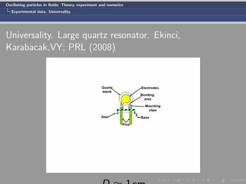
Experimental data. Universality.
Universality. Large quartz resonator. Ekinci,Karabacak,VY; PRL (2008)
Base
Mountingclips
Bondingarea
ElectrodesQuartzblank
Seal
Pins
D ≈ 1cm

Oscillating particles in fluids: Theory, experiment and numerics
Experimental data. Universality.
1/Q vs pressure for different ω
Oscillating particles in fluids: Theory, experiment and numerics
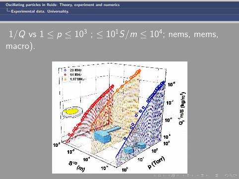
Experimental data. Universality.
1/Q vs 1 ≤ p ≤ 103 ; ≤ 101S/m ≤ 104; nems, mems,macro).

Oscillating particles in fluids: Theory, experiment and numerics
Experimental data. Universality.
1/Q vs 10 ≤ p ≤ 103 ; ≤ 101S/m ≤ 104;NEMS, MEMS, Quartz (macro).
Oscillating particles in fluids: Theory, experiment and numerics
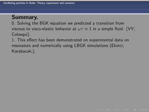
Summary.0. Solving the BGK equation we predicted a transition fromviscous to visco-elastic behavior at ωτ ≈ 1 in a simple fluid. (VY;Colosqui).1. This effect has been demonstrated on experimental data onresonators and numerically using LBGK simulations (Ekinci;Karabacak;).
Oscillating particles in fluids: Theory, experiment and numerics
2. Size of the device in a vast range 10−4 ≤ L ≤ 1cm does notenter the results represented as a function of x = ωτ . This pointsto the universality which is a much broader class than thewell-known SIMILARITY.3. The transition is due to formation of propagating shear wave inthe Knudsen layer. Is it a new physics emerged from LBM?(Mandelshtam/ Leontovich (chem reactions), Boon (relaxation dueto polymers etc)...
I do not know any work showing thisphenomenon in simple flows. Are you?

Oscillating particles in fluids: Theory, experiment and numerics
3. We have found a UNIVERSALITY in the entire range0 ≤ ωτ ≤ ∞
u = Uφ(r
L,λ
L, ωτ,Re)
with the scaling function f (x) derived from kinetic equation.

Oscillating particles in fluids: Theory, experiment and numerics
4. LBGK simulations agree with experimental results. (non-trivialoutcome).
5. The transition is general U(x , 0) = U sin(ky). (Colosqui et alPhys. Pluids. (January))

Oscillating particles in fluids: Theory, experiment and numerics
6. Bodies of finite size (Colosqui)7. Boundary conditions; slip -no-slip.

Oscillating particles in fluids: Theory, experiment and numerics
Different geometries. Different scales.
Oscillating particles in fluids: Theory, experiment and numerics
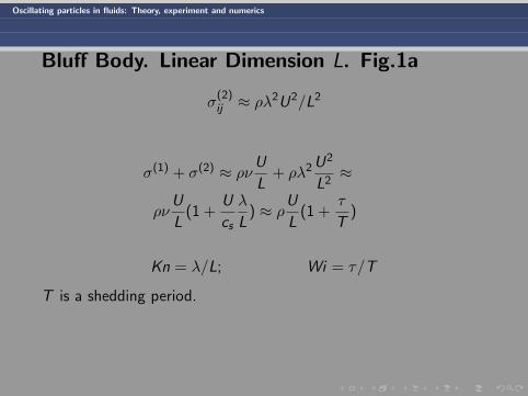
Bluff Body. Linear Dimension L. Fig.1a
σ(2)ij ≈ ρλ
2U2/L2
σ(1) + σ(2) ≈ ρνU
L+ ρλ2
U2
L2≈
ρνU
L(1 +
U
cs
λ
L) ≈ ρU
L(1 +
τ
T)
Kn = λ/L; Wi = τ/T
T is a shedding period.

Oscillating particles in fluids: Theory, experiment and numerics
Boundary Layer.
σ(1) ≈ ρν ∂u
∂y≈ ρcsλ
U
δ(x)
σ(2) ∝ ∂ui
∂xα
∂uj
∂xα= 0
σ(2) ≈ ρλ2∂uu∇ · u ≈ ρλ2 U2
xδ
σ(1) + σ(2) ≈ ρcsλU
δ(1 +
λ2
δ2)

Oscillating particles in fluids: Theory, experiment and numerics
In the Stokes problem

Oscillating particles in fluids: Theory, experiment and numerics
Future: 1. This may be a huge area with applications in chemicalengineering, combustion, bio/medical engineering etc. Based onwhat we know LBM may become the most important tool......
Oscillating particles in fluids: Theory, experiment and numerics
TIME The parameter τ i: s a time scale characterizing return of aninitially perturbed system to thermodynamic equilibrium. If, forexample, at time t = 0, a small volume fraction of a gas is locallyperturbed from thermodynamic equilibrium by an excess energy∆E (local heat release, for example), due to intermolecularcollisions or collisions with the walls of the vessel, this localperturbation (inhomogeneity) must disappear on a time-scale τ .The first-principle derivation of this parameter, requiring fulldescription of all microscopic details of interactions is very difficultand, in general, is impossible. It is especially hard if relaxationprocess involves interactions with the solid bodies and excitationsof phonons and other internal degrees of freedom by a gasmolecule impacting the surface. It is clear that in the case of aflow generated by an oscillating solid surface, it is the gas -surfaceinteraction which is responsible for the dissipation process. Forideal gas of the number density n colliding with the wall:

Oscillating particles in fluids: Theory, experiment and numerics
τ ≈ λcs ∝csσn∝ kBθ
32
σp≡ I
p
where the cross-section σ includes all microscopic information. It iseasy to estimate the relaxation time in a bulk of a gas of hardspheres of diameter d where σ ∝ d2. For a nitrogen gas it givesτ ≈ 180× 10−9sec . The relaxation time can experimentally beestablished from the relation ωτ ≈ 1 marking the bending in adissipation curve γ(τω (See Fig. [XX]. The observed dependenceτ ∝ 1/p is shown on Fig. [XX]. Our experimental data giveI ≈ 1850− 1500 for nanocantilevers and nanobeams andI ≈ 400− 500 for the quartz resonators with aluminum - coveredsurface. The fact that all silicon -based nanodevices can becharcterized by the same magnitude of coefficientI ≈ I = 1850× 10−9sec points to the microscopic details ofgas-surface interaction as an important factor.