Optimization - Purdue University - Department of ...vishy/introml/notes/Optimization.pdf · 5...
52
5 Optimization Optimization plays an increasingly important role in machine learning. For instance, many machine learning algorithms minimize a regularized risk functional: min f J (f ) := λΩ(f )+ R emp (f )� (5.1) with the empirical risk R emp (f ) := 1 m m � i=1 l(f (x i )�y i ). (5.2) Here x i are the training instances and y i are the corresponding labels. l the loss function measures the discrepancy between y and the predictions f (x i ). Finding the optimal f involves solving an optimization problem. This chapter provides a self-contained overview of some basic concepts and tools from optimization, especially geared towards solving machine learning problems. In terms of concepts, we will cover topics related to convexity, duality, and Lagrange multipliers. In terms of tools, we will cover a variety of optimization algorithms including gradient descent, stochastic gradient descent, Newton’s method, and Quasi-Newton methods. We will also look at some specialized algorithms tailored towards solving Linear Programming and Quadratic Programming problems which often arise in machine learning problems. 5.1 Preliminaries Minimizing an arbitrary function is, in general, very difficult, but if the ob- jective function to be minimized is convex then things become considerably simpler. As we will see shortly, the key advantage of dealing with convex functions is that a local optima is also the global optima. Therefore, well developed tools exist to find the global minima of a convex function. Conse- quently, many machine learning algorithms are now formulated in terms of convex optimization problems. We briefly review the concept of convex sets and functions in this section. 129
Transcript of Optimization - Purdue University - Department of ...vishy/introml/notes/Optimization.pdf · 5...
5
Optimization
Optimization plays an increasingly important role in machine learning. For
instance, many machine learning algorithms minimize a regularized risk
functional:
minf
J(f) := λΩ(f) +Remp(f)� (5.1)
with the empirical risk
Remp(f) :=1
m
m�
i=1
l(f(xi)� yi). (5.2)
Here xi are the training instances and yi are the corresponding labels. l the
loss function measures the discrepancy between y and the predictions f(xi).
Finding the optimal f involves solving an optimization problem.
This chapter provides a self-contained overview of some basic concepts and
tools from optimization, especially geared towards solving machine learning
problems. In terms of concepts, we will cover topics related to convexity,
duality, and Lagrange multipliers. In terms of tools, we will cover a variety
of optimization algorithms including gradient descent, stochastic gradient
descent, Newton’s method, and Quasi-Newton methods. We will also look
at some specialized algorithms tailored towards solving Linear Programming
and Quadratic Programming problems which often arise in machine learning
problems.
5.1 Preliminaries
Minimizing an arbitrary function is, in general, very difficult, but if the ob-
jective function to be minimized is convex then things become considerably
simpler. As we will see shortly, the key advantage of dealing with convex
functions is that a local optima is also the global optima. Therefore, well
developed tools exist to find the global minima of a convex function. Conse-
quently, many machine learning algorithms are now formulated in terms of
convex optimization problems. We briefly review the concept of convex sets
and functions in this section.
129
130 5 Optimization
5.1.1 Convex Sets
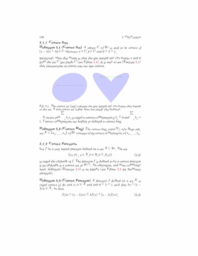
Definition 5.1 �Convex Set) A subset C of Rn is said to be convex if
(1− λ)x+ λy ∈ C whenever x ∈ C� y ∈ C and 0 < λ < 1.
Intuitively, what this means is that the line joining any two points x and y
from the set C lies inside C (see Figure 5.1). It is easy to see (Exercise 5.1)
that intersections of convex sets are also convex.
Fig. 5.1. The convex set (left) contains the line joining any two points that belongto the set. A non-convex set (right) does not satisfy this property.
A vector sum�
i λixi is called a convex combination if λi ≥ 0 and�
i λi =
1. Convex combinations are helpful in defining a convex hull:
Definition 5.2 �Convex Hull) The convex hull, conv(X), of a finite sub-
set X = {x1� . . . � xn} of Rn consists of all convex combinations of x1� . . . � xn.
5.1.2 Convex Functions
Let f be a real valued function defined on a set X ⊂ Rn. The set
{(x� µ) : x ∈ X�µ ∈ R� µ ≥ f(x)} (5.3)
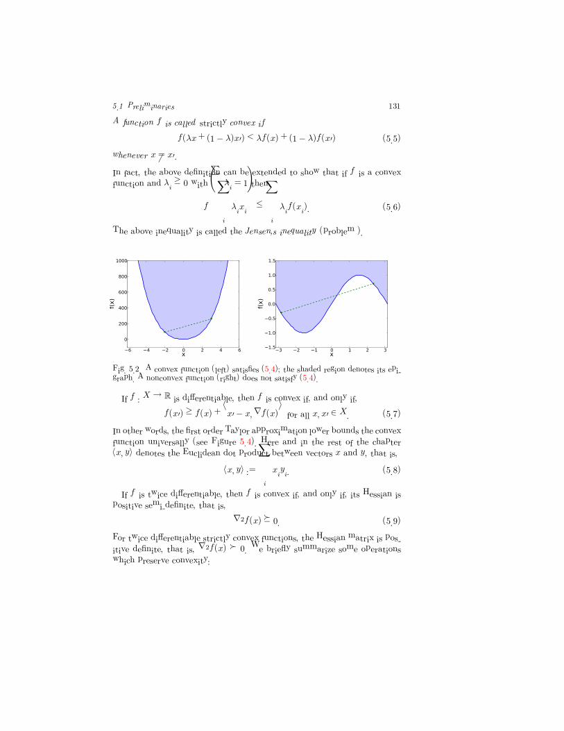
is called the epigraph of f . The function f is defined to be a convex function
if its epigraph is a convex set in Rn+1. An equivalent, and more commonly
used, definition (Exercise 5.5) is as follows (see Figure 5.2 for geometric
intuition):
Definition 5.3 �Convex Function) A function f defined on a set X is
called convex if, for any x� x� ∈ X and any 0 < λ < 1 such that λx + (1 −
λ)x� ∈ X, we have
f(λx+ (1− λ)x�) ≤ λf(x) + (1− λ)f(x�). (5.4)
5.1 Preliminaries 131
A function f is called strictly convex if
f(λx+ (1− λ)x�) < λf(x) + (1− λ)f(x�) (5.5)
whenever x �= x�.
In fact, the above definition can be extended to show that if f is a convex
function and λi ≥ 0 with�
i λi = 1 then
f
��
i
λixi
�
≤�
i
λif(xi). (5.6)
The above inequality is called the Jensen’s inequality (problem ).
� � � � � � �
�
�
���
���
���
���
����
����
� � � � � � �
�
���
���
���
���
���
���
�������
Fig. 5.2. A convex function (left) satisfies (5.4); the shaded region denotes its epi-graph. A nonconvex function (right) does not satisfy (5.4).
If f : X → R is differentiable, then f is convex if, and only if,
f(x�) ≥ f(x) +�x� − x�∇f(x)
�for all x� x� ∈ X. (5.7)
In other words, the first order Taylor approximation lower bounds the convex
function universally (see Figure 5.4). Here and in the rest of the chapter
�x� y� denotes the Euclidean dot product between vectors x and y, that is,
�x� y� :=�
i
xiyi. (5.8)
If f is twice differentiable, then f is convex if, and only if, its Hessian is
positive semi-definite, that is,
∇2f(x) � 0. (5.9)
For twice differentiable strictly convex functions, the Hessian matrix is pos-
itive definite, that is, ∇2f(x) � 0. We briefly summarize some operations
which preserve convexity:
132 5 Optimization
Addition If f1 and f2 are convex, then f1 + f2 is also convex.Scaling If f is convex, then αf is convex for α > 0.
Affine Transform If f is convex, then g(x) = f(Ax+ b) for some matrixA and vector b is also convex.
Adding a Linear Function If f is convex, then g(x) = f(x)+�a� x� for some vectora is also convex.
Subtracting a Linear Function If f is convex, then g(x) = f(x)−�a� x� for some vectora is also convex.
Pointwise Maximum If fi are convex, then g(x) = maxi fi(x) is also convex.Scalar Composition If f(x) = h(g(x)), then f is convex if a) g is convex,
and h is convex, non-decreasing or b) g is concave, andh is convex, non-increasing.
-3-2
-1 0
1 2
3-3
-2
-1
0
1
2
3
0 2 4 6 8
10 12 14 16 18
-3-2-1 0 1 2 3-3
-2
-1
0
1
2
3
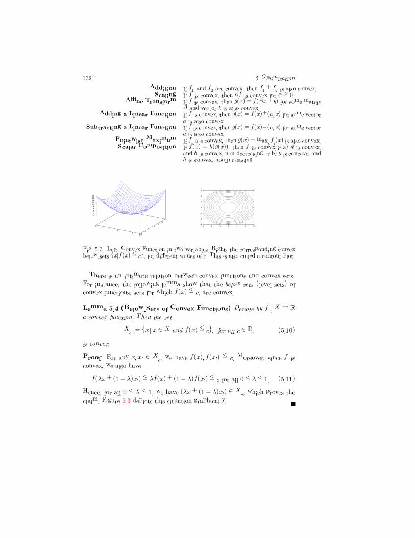
Fig. 5.3. Left: Convex Function in two variables. Right: the corresponding convexbelow-sets {x|f(x) ≤ c}, for different values of c. This is also called a contour plot.
There is an intimate relation between convex functions and convex sets.
For instance, the following lemma show that the below sets (level sets) of
convex functions, sets for which f(x) ≤ c, are convex.
Lemma 5.4 �Below-Sets of Convex Functions) Denote by f : X → R
a convex function. Then the set
Xc := {x |x ∈ X and f(x) ≤ c}� for all c ∈ R� (5.10)
is convex.
Proof For any x� x� ∈ Xc, we have f(x)� f(x�) ≤ c. Moreover, since f is
convex, we also have
f(λx+ (1− λ)x�) ≤ λf(x) + (1− λ)f(x�) ≤ c for all 0 < λ < 1. (5.11)
Hence, for all 0 < λ < 1, we have (λx + (1 − λ)x�) ∈ Xc, which proves the
claim. Figure 5.3 depicts this situation graphically.
5.1 Preliminaries 133
As we hinted in the introduction of this chapter, minimizing an arbitrary
function on a (possibly not even compact) set of arguments can be a difficult
task, and will most likely exhibit many local minima. In contrast, minimiza-
tion of a convex objective function on a convex set exhibits exactly one global
minimum. We now prove this property.
Theorem 5.5 �Minima on Convex Sets) If the convex function f : X →
R attains its minimum, then the set of x ∈ X, for which the minimum value
is attained, is a convex set. Moreover, if f is strictly convex, then this set
contains a single element.
Proof Denote by c the minimum of f on X. Then the set Xc := {x|x ∈
X and f(x) ≤ c} is clearly convex.
If f is strictly convex, then for any two distinct x� x� ∈ Xc and any 0 <
λ < 1 we have
f(λx+ (1− λ)x�) < λf(x) + (1− λ)f(x�) = λc+ (1− λ)c = c�
which contradicts the assumption that f attains its minimum on Xc. There-
fore Xc must contain only a single element.
As the following lemma shows, the minimum point can be characterized
precisely.
Lemma 5.6 Let f : X → R be a differentiable convex function. Then x is
a minimizer of f , if, and only if,�x� − x�∇f(x)
�≥ 0 for all x�. (5.12)
Proof To show the forward implication, suppose that x is the optimum
but (5.12) does not hold, that is, there exists an x� for which�x� − x�∇f(x)
�< 0.
Consider the line segment z(λ) = (1 − λ)x + λx�, with 0 < λ < 1. Since X
is convex, z(λ) lies in X. On the other hand,
d
dλf(z(λ))
����λ=0
=�x� − x�∇f(x)
�< 0�
which shows that for small values of λ we have f(z(λ)) < f(x), thus showing
that x is not optimal.
The reverse implication follows from (5.7) by noting that f(x�) ≥ f(x),
whenever (5.12) holds.
134 5 Optimization
One way to ensure that (5.12) holds is to set ∇f(x) = 0. In other words,
minimizing a convex function is equivalent to finding a x such that ∇f(x) =
0. Therefore, the first order conditions are both necessary and sufficient
when minimizing a convex function.
5.1.3 Subgradients
So far, we worked with differentiable convex functions. The subgradient is a
generalization of gradients appropriate for convex functions, including those
which are not necessarily smooth.
Definition 5.7 �Subgradient) Suppose x is a point where a convex func-
tion f is finite. Then a subgradient is the normal vector of any tangential
supporting hyperplane of f at x. Formally µ is called a subgradient of f at
x if, and only if,
f(x�) ≥ f(x) +�x� − x� µ
�for all x�. (5.13)
The set of all subgradients at a point is called the subdifferential, and is de-
noted by ∂xf(x). If this set is not empty then f is said to be subdifferentiable
at x. On the other hand, if this set is a singleton then, the function is said
to be differentiable at x. In this case we use ∇f(x) to denote the gradient
of f . Convex functions are subdifferentiable everywhere in their domain. We
now state some simple rules of subgradient calculus:
Addition ∂x(f1(x) + f2(x)) = ∂xf1(x) + ∂xf2(x)Scaling ∂xαf(x) = α∂xf(x), for α > 0
Affine Transform If g(x) = f(Ax + b) for some matrix A and vector b,then ∂xg(x) = A�∂yf(y).
Pointwise Maximum If g(x) = maxi fi(x) then ∂g(x) = conv(∂xfi�) wherei� ∈ argmaxi fi(x).
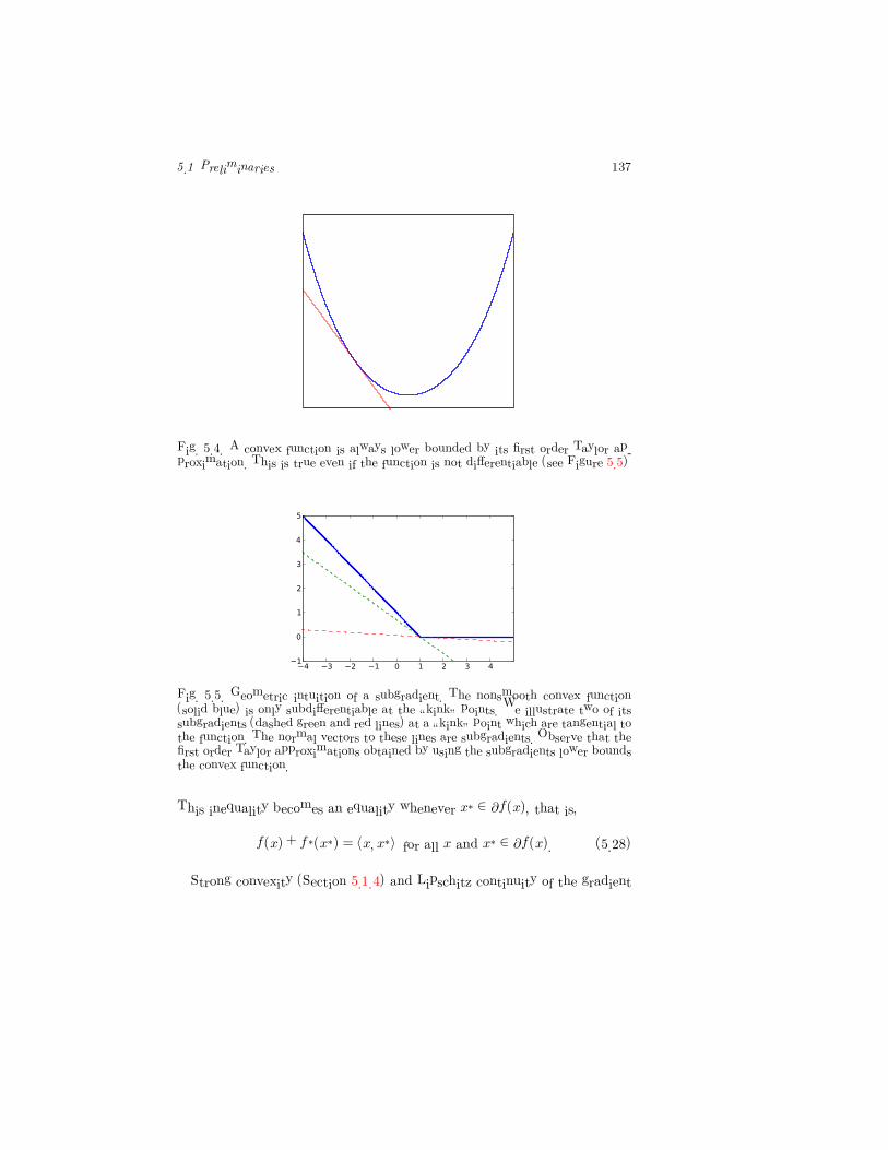
The definition of a subgradient can also be understood geometrically. As
illustrated by Figure 5.4, a differentiable convex function is always lower
bounded by its first order Taylor approximation. This concept can be ex-
tended to non-smooth functions via subgradients, as Figure 5.5 shows.
By using more involved concepts, the proof of Lemma 5.6 can be extended
to subgradients. In this case, minimizing a convex nonsmooth function en-
tails finding a x such that 0 ∈ ∂f(x).
5.1 Preliminaries 135
5.1.4 Strongly Convex Functions
When analyzing optimization algorithms, it is sometimes easier to work with
strongly convex functions, which generalize the definition of convexity.
Definition 5.8 �Strongly Convex Function) A convex function f is σ-
strongly convex if, and only if, there exists a constant σ > 0 such that the
function f(x)− σ2 �x�
2 is convex.
The constant σ is called the modulus of strong convexity of f . If f is twice
differentiable, then there is an equivalent, and perhaps easier, definition of
strong convexity: f is strongly convex if there exists a σ such that
∇2f(x) � σI. (5.14)
In other words, the smallest eigenvalue of the Hessian of f is uniformly
lower bounded by σ everywhere. Some important examples of strongly con-
vex functions include:
Example 5.1 �Squared Euclidean Norm) The function f(x) = λ2 �x�
2
is λ-strongly convex.
Example 5.2 �Negative Entropy) Let Δn = {x s.t.�
i xi = 1 and xi ≥ 0}
be the n dimensional simplex, and f : Δn → R be the negative entropy:
f(x) =�
i
xi log xi. (5.15)
Then f is 1-strongly convex with respect to the �·�1 norm on the simplex
(see Problem 5.7).
If f is a σ-strongly convex function then one can show the following prop-
erties (Exercise 5.8). Here x� x� are arbitrary and µ ∈ ∂f(x) and µ� ∈ ∂f(x�).
f(x�) ≥ f(x) +�x� − x� µ
�+
σ
2
��x� − x
��2 (5.16)
f(x�) ≤ f(x) +�x� − x� µ
�+
1
2σ
��µ� − µ
��2 (5.17)
�x− x�� µ− µ�
�≥ σ
��x− x�
��2 (5.18)
�x− x�� µ− µ�
�≤
1
σ
��µ− µ�
��2 . (5.19)
136 5 Optimization
5.1.5 Convex Functions with Lipschitz Continous Gradient
A somewhat symmetric concept to strong convexity is the Lipschitz conti-
nuity of the gradient. As we will see later they are connected by Fenchel
duality.
Definition 5.9 �Lipschitz Continuous Gradient) A differentiable con-
vex function f is said to have a Lipschitz continuous gradient, if there exists
a constant L > 0, such that��∇f(x)−∇f(x�)
�� ≤ L
��x− x�
�� ∀x� x�. (5.20)
As before, if f is twice differentiable, then there is an equivalent, and perhaps
easier, definition of Lipschitz continuity of the gradient: f has a Lipschitz
continuous gradient strongly convex if there exists a L such that
LI � ∇2f(x). (5.21)
In other words, the largest eigenvalue of the Hessian of f is uniformly upper
bounded by L everywhere. If f has a Lipschitz continuous gradient with
modulus L, then one can show the following properties (Exercise 5.9).
f(x�) ≤ f(x) +�x� − x�∇f(x)
�+
L
2
��x− x�
��2 (5.22)
f(x�) ≥ f(x) +�x� − x�∇f(x)
�+
1
2L
��∇f(x)−∇f(x�)
��2 (5.23)
�x− x��∇f(x)−∇f(x�)
�≤ L
��x− x�
��2 (5.24)
�x− x��∇f(x)−∇f(x�)
�≥
1
L
��∇f(x)−∇f(x�)
��2 . (5.25)
5.1.6 Fenchel Duality
The Fenchel conjugate of a function f is given by
f∗(x∗) = supx{�x� x∗� − f(x)} . (5.26)
Even if f is not convex, the Fechel conjugate which is written as a supremum
over linear functions is always convex. Some rules for computing Fenchel
duals are summarized in Table 5.1.6. If f is convex and its epigraph (5.3) is
a closed convex set, then f∗∗ = f . If f and f∗ are convex, then they satisfy
the so-called Fenchel-Young inequality
f(x) + f∗(x∗) ≥ �x� x∗� for all x� x∗. (5.27)
5.1 Preliminaries 137
Fig. 5.4. A convex function is always lower bounded by its first order Taylor ap-proximation. This is true even if the function is not differentiable (see Figure 5.5)
� � � � � � � � ��
�
�
�
�
�
�
Fig. 5.5. Geometric intuition of a subgradient. The nonsmooth convex function(solid blue) is only subdifferentiable at the “kink” points. We illustrate two of itssubgradients (dashed green and red lines) at a “kink” point which are tangential tothe function. The normal vectors to these lines are subgradients. Observe that thefirst order Taylor approximations obtained by using the subgradients lower boundsthe convex function.
This inequality becomes an equality whenever x∗ ∈ ∂f(x), that is,
f(x) + f∗(x∗) = �x� x∗� for all x and x∗ ∈ ∂f(x). (5.28)
Strong convexity (Section 5.1.4) and Lipschitz continuity of the gradient
138 5 Optimization
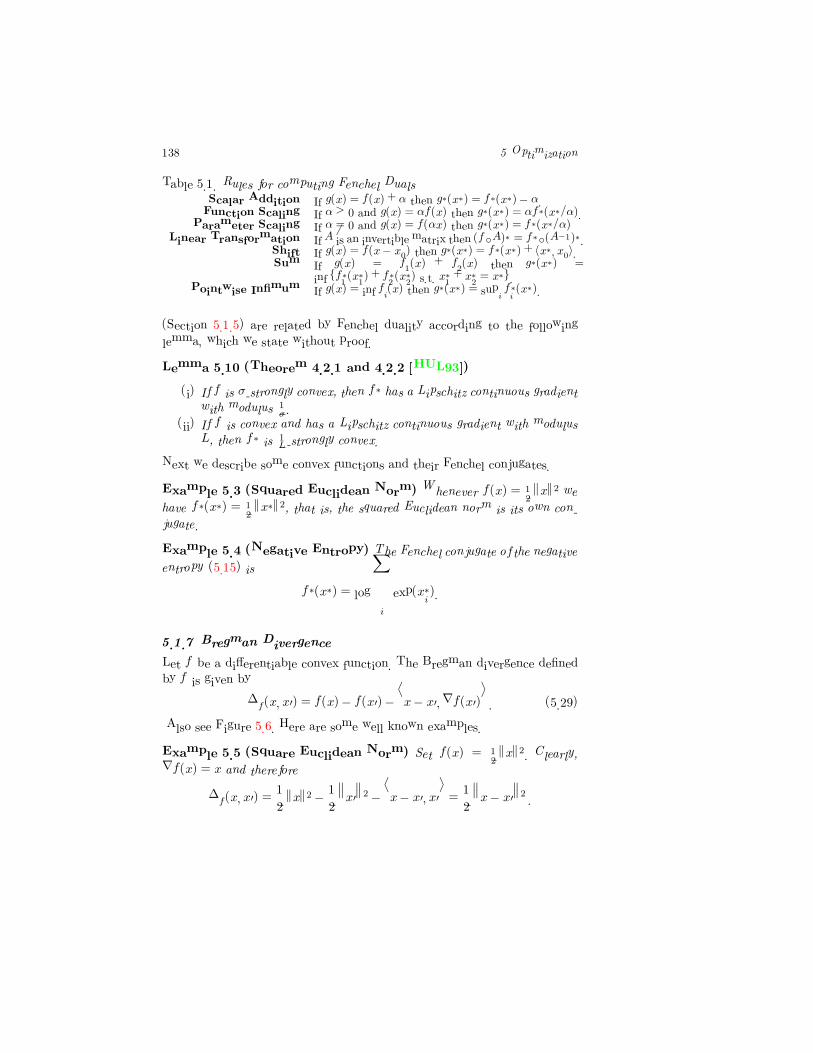
Table 5.1. Rules for computing Fenchel DualsScalar Addition If g(x) = f(x) + α then g∗(x∗) = f∗(x∗)− α.Function Scaling If α > 0 and g(x) = αf(x) then g∗(x∗) = αf∗(x∗/α).Parameter Scaling If α �= 0 and g(x) = f(αx) then g∗(x∗) = f∗(x∗/α)
Linear Transformation If A is an invertible matrix then (f ◦A)∗ = f∗◦(A�1)∗.Shift If g(x) = f(x− x0) then g∗(x∗) = f∗(x∗) + �x∗� x0�.Sum If g(x) = f1(x) + f2(x) then g∗(x∗) =
inf {f∗1 (x∗
1) + f∗2 (x∗
2) s.t. x∗
1 + x∗2 = x∗}.Pointwise Infimum If g(x) = inf fi(x) then g∗(x∗) = supi f
∗
i (x∗).
(Section 5.1.5) are related by Fenchel duality according to the following
lemma, which we state without proof.
Lemma 5.10 �Theorem 4.2.1 and 4.2.2 [HUL93])
(i) If f is σ-strongly convex, then f∗ has a Lipschitz continuous gradient
with modulus 1σ .
(ii) If f is convex and has a Lipschitz continuous gradient with modulus
L, then f∗ is 1L -strongly convex.
Next we describe some convex functions and their Fenchel conjugates.
Example 5.3 �Squared Euclidean Norm) Whenever f(x) = 12 �x�
2 we
have f∗(x∗) = 12 �x
∗�2, that is, the squared Euclidean norm is its own con-
jugate.
Example 5.4 �Negative Entropy) The Fenchel conjugate of the negative
entropy (5.15) is
f∗(x∗) = log�
i
exp(x∗i ).
5.1.7 Bregman Divergence
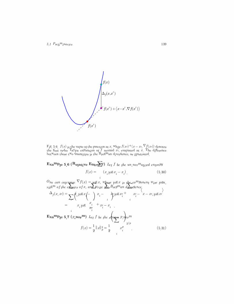
Let f be a differentiable convex function. The Bregman divergence defined
by f is given by
Δf (x� x�) = f(x)− f(x�)−
�x− x��∇f(x�)
�. (5.29)
Also see Figure 5.6. Here are some well known examples.
Example 5.5 �Square Euclidean Norm) Set f(x) = 12 �x�
2. Clearly,
∇f(x) = x and therefore
Δf (x� x�) =
1
2�x�2 −
1
2
��x�
��2 −
�x− x�� x�
�=
1
2
��x− x�
��2 .
5.1 Preliminaries 139
���� �
����
���� � ������ ������ �
�
������� �
Fig. 5.6. f(x) is the value of the function at x, while f(x�)+�x− x��∇f(x�)� denotesthe first order Taylor expansion of f around x�, evaluated at x. The differencebetween these two quantities is the Bregman divergence, as illustrated.
Example 5.6 �Relative Entropy) Let f be the un-normalized entropy
f(x) =�
i
(xi log xi − xi) . (5.30)
One can calculate ∇f(x) = log x, where log x is the component wise loga-
rithm of the entries of x, and write the Bregman divergence
Δf (x� x�) =
�
i
xi log xi −�
i
xi −�
i
x�i log x�i +
�
i
x�i −�x− x�� log x�
�
=�
i
�
xi log
�xix�i
�
+ x�i − xi
�
.
Example 5.7 �p-norm) Let f be the square p-norm
f(x) =1
2�x�2p =
1
2
��
i
xpi
�2/p
. (5.31)
140 5 Optimization
We say that the q-norm is dual to the p-norm whenever 1p +
1q = 1. One can
verify (Problem 5.12) that the i-th component of the gradient ∇f(x) is
∇xif(x) =
sign(xi) |xi|p−1
�x�p−2p
. (5.32)
The corresponding Bregman divergence is
Δf (x� x�) =
1
2�x�2p −
1
2
��x�
��2p−
�
i
(xi − x�i)sign(x�i) |x
�i|p−1
�x��p−2p
.
The following properties of the Bregman divergence immediately follow:
• Δf (x� x�) is convex in x.
• Δf (x� x�) ≥ 0.
• Δf may not be symmetric, that is, in general Δf (x� x�) �= Δf (x
�� x).
• ∇xΔf (x� x�) = ∇f(x)−∇f(x�).
The next lemma establishes another important property.
Lemma 5.11 The Bregman divergence (5.29) defined by a differentiable
convex function f satisfies
Δf (x� y) + Δf (y� z)−Δf (x� z) = �∇f(z)−∇f(y)� x− y� . (5.33)
Proof
Δf (x� y) + Δf (y� z) = f(x)− f(y)− �x− y�∇f(y)�+ f(y)− f(z)− �y − z�∇f(z)�
= f(x)− f(z)− �x− y�∇f(y)� − �y − z�∇f(z)�
= Δf (x� z) + �∇f(z)−∇f(y)� x− y� .
5.2 Unconstrained Smooth Convex Minimization
In this section we will describe various methods to minimize a smooth convex
objective function.
5.2.1 Minimizing a One-Dimensional Convex Function
As a warm up let us consider the problem of minimizing a smooth one di-
mensional convex function J : R → R in the interval [L�U ]. This seemingly
5.2 Unconstrained Smooth Convex Minimization 141
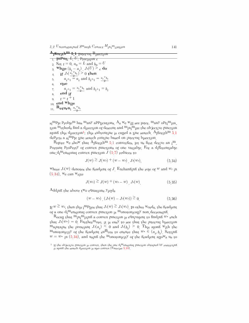
Algorithm 5.1 Interval Bisection
1: Input: L, U , precision �
2: Set t = 0, a0 = L and b0 = U
3: while (bt − at) · J�(U) > � do
4: if J �(at+bt
2 ) > 0 then
5: at+1 = at and bt+1 =at+bt
2
6: else
7: at+1 =at+bt
2 and bt+1 = bt8: end if
9: t = t+ 1
10: end while
11: Return: at+bt
2
simple problem has many applications. As we will see later, many optimiza-
tion methods find a direction of descent and minimize the objective function
along this direction1; this subroutine is called a line search. Algorithm 5.1
depicts a simple line search routine based on interval bisection.
Before we show that Algorithm 5.1 converges, let us first derive an im-
portant property of convex functions of one variable. For a differentiable
one-dimensional convex function J (5.7) reduces to
J(w) ≥ J(w�) + (w − w�) · J �(w�)� (5.34)
where J �(w) denotes the gradient of J . Exchanging the role of w and w� in
(5.34), we can write
J(w�) ≥ J(w) + (w� − w) · J �(w). (5.35)
Adding the above two equations yields
(w − w�) · (J �(w)− J �(w�)) ≥ 0. (5.36)
If w ≥ w�, then this implies that J �(w) ≥ J �(w�). In other words, the gradient
of a one dimensional convex function is monotonically non-decreasing.
Recall that minimizing a convex function is equivalent to finding w∗ such
that J �(w∗) = 0. Furthermore, it is easy to see that the interval bisection
maintains the invariant J �(at) < 0 and J �(bt) > 0. This along with the
monotonicity of the gradient suffices to ensure that w∗ ∈ (at� bt). Setting
w = w∗ in (5.34), and using the monotonicity of the gradient allows us to
1 If the objective function is convex, then the one dimensional function obtained by restrictingit along the search direction is also convex (Exercise 5.10).
142 5 Optimization
write for any w� ∈ (at� bt)
J(w�)− J(w∗) ≤ (w� − w∗) · J �(w�) ≤ (bt − at) · J�(U). (5.37)
Since we halve the interval (at� bt) at every iteration, it follows that (bt−at) =
(U − L)/2t. Therefore
J(w�)− J(w∗) ≤(U − L) · J �(U)
2t� (5.38)
for all w� ∈ (at� bt). In other words, to find an �-accurate solution, that is,
J(w�)− J(w∗) ≤ � we only need log(U −L) + log J �(U) + log(1/�) < t itera-
tions. An algorithm which converges to an � accurate solution in O(log(1/�))
iterations is said to be linearly convergent.
For multi-dimensional objective functions, one cannot rely on the mono-
tonicity property of the gradient. Therefore, one needs more sophisticated
optimization algorithms, some of which we now describe.
5.2.2 Coordinate Descent
Coordinate descent is conceptually the simplest algorithm for minimizing a
multidimensional smooth convex function J : Rn → R. At every iteration
select a coordinate, say i, and update
wt+1 = wt − ηtei. (5.39)
Here ei denotes the i-th basis vector, that is, a vector with one at the i-th co-
ordinate and zeros everywhere else, while ηt ∈ R is a non-negative scalar step
size. One could, for instance, minimize the one dimensional convex function
J(wt− ηei) to obtain the stepsize ηt. The coordinates can either be selected
cyclically, that is, 1� 2� . . . � n� 1� 2� . . . or greedily, that is, the coordinate which
yields the maximum reduction in function value.
Even though coordinate descent can be shown to converge if J has a Lip-
schitz continuous gradient [LT92], in practice it can be quite slow. However,
if a high precision solution is not required, as is the case in some machine
learning applications, coordinate descent is often used because a) the cost
per iteration is very low and b) the speed of convergence may be acceptable
especially if the variables are loosely coupled.
5.2.3 Gradient Descent
Gradient descent (also widely known as steepest descent) is an optimization
technique for minimizing multidimensional smooth convex objective func-
tions of the form J : Rn → R. The basic idea is as follows: Given a location
5.2 Unconstrained Smooth Convex Minimization 143
wt at iteration t, compute the gradient ∇J(wt), and update
wt+1 = wt − ηt∇J(wt)� (5.40)
where ηt is a scalar stepsize. See Algorithm 5.2 for details. Different variants
of gradient descent depend on how ηt is chosen:
Exact Line Search: Since J(wt − η∇J(wt)) is a one dimensional convex
function in η, one can use the Algorithm 5.1 to compute:
ηt = argminη
J(wt − η∇J(wt)). (5.41)
Instead of the simple bisecting line search more sophisticated line searches
such as the More-Thuente line search or the golden bisection rule can also
be used to speed up convergence (see [NW99] Chapter 3 for an extensive
discussion).
Inexact Line Search: Instead of minimizing J(wt − η∇J(wt)) we could
simply look for a stepsize which results in sufficient decrease in the objective
function value. One popular set of sufficient decrease conditions is the Wolfe
conditions
J(wt+1) ≤ J(wt) + c1ηt �∇J(wt)� wt+1 − wt� (sufficient decrease) (5.42)
�∇J(wt+1)� wt+1 − wt� ≥ c2 �∇J(wt)� wt+1 − wt� (curvature) (5.43)
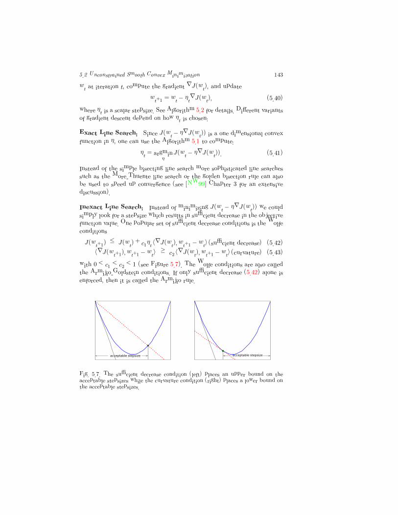
with 0 < c1 < c2 < 1 (see Figure 5.7). The Wolfe conditions are also called
the Armijio-Goldstein conditions. If only sufficient decrease (5.42) alone is
enforced, then it is called the Armijio rule.
������������������� �������������������
Fig. 5.7. The sufficient decrease condition (left) places an upper bound on theacceptable stepsizes while the curvature condition (right) places a lower bound onthe acceptable stepsizes.
144 5 Optimization
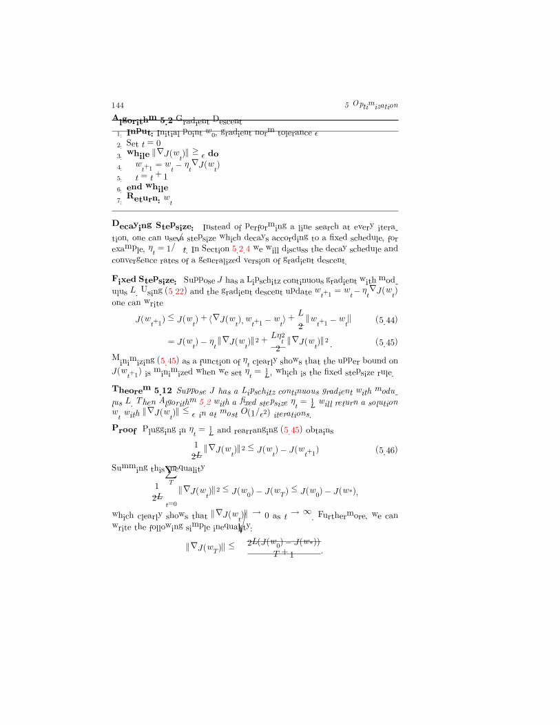
Algorithm 5.2 Gradient Descent
1: Input: Initial point w0, gradient norm tolerance �
2: Set t = 0
3: while �∇J(wt)� ≥ � do
4: wt+1 = wt − ηt∇J(wt)
5: t = t+ 1
6: end while
7: Return: wt
Decaying Stepsize: Instead of performing a line search at every itera-
tion, one can use a stepsize which decays according to a fixed schedule, for
example, ηt = 1/√t. In Section 5.2.4 we will discuss the decay schedule and
convergence rates of a generalized version of gradient descent.
Fixed Stepsize: Suppose J has a Lipschitz continuous gradient with mod-
ulus L. Using (5.22) and the gradient descent update wt+1 = wt− ηt∇J(wt)
one can write
J(wt+1) ≤ J(wt) + �∇J(wt)� wt+1 − wt�+L
2�wt+1 − wt� (5.44)
= J(wt)− ηt �∇J(wt)�2 +
Lη2t2
�∇J(wt)�2 . (5.45)
Minimizing (5.45) as a function of ηt clearly shows that the upper bound on
J(wt+1) is minimized when we set ηt =1L , which is the fixed stepsize rule.
Theorem 5.12 Suppose J has a Lipschitz continuous gradient with modu-
lus L. Then Algorithm 5.2 with a fixed stepsize ηt =1L will return a solution
wt with �∇J(wt)� ≤ � in at most O(1/�2) iterations.
Proof Plugging in ηt =1L and rearranging (5.45) obtains
1
2L�∇J(wt)�
2 ≤ J(wt)− J(wt+1) (5.46)
Summing this inequality
1
2L
T�
t=0
�∇J(wt)�2 ≤ J(w0)− J(wT ) ≤ J(w0)− J(w∗)�
which clearly shows that �∇J(wt)� → 0 as t → ∞. Furthermore, we can
write the following simple inequality:
�∇J(wT )� ≤
�2L(J(w0)− J(w∗))
T + 1.
5.2 Unconstrained Smooth Convex Minimization 145
Solving for�
2L(J(w0)− J(w∗))
T + 1= �
shows that T is O(1/�2) as claimed.
If in addition to having a Lipschitz continuous gradient, if J is σ-strongly
convex, then more can be said. First, one can translate convergence in
�∇J(wt)� to convergence in function values. Towards this end, use (5.17) to
write
J(wt) ≤ J(w∗) +1
2σ�∇J(wt)�
2 .
Therefore, it follows that whenever �∇J(wt)� < � we have J(wt)− J(w∗) <
�2/2σ. Furthermore, we can strengthen the rates of convergence.
Theorem 5.13 Assume everything as in Theorem 5.12. Moreover assume
that J is σ-strongly convex, and let c := 1 − σL . Then J(wt) − J(w∗) ≤ �
after at most
log((J(w0)− J(w∗))/�)
log(1/c)(5.47)
iterations.
Proof Combining (5.46) with �∇J(wt)�2 ≥ 2σ(J(wt)− J(w∗)), and using
the definition of c one can write
c(J(wt)− J(w∗)) ≥ J(wt+1)− J(w∗).
Applying the above equation recursively
cT (J(w0)− J(w∗)) ≥ J(wT )− J(w∗).
Solving for
� = cT (J(w0)− J(w∗))
and rearranging yields (5.47).
When applied to practical problems which are not strongly convex gra-
dient descent yields a low accuracy solution within a few iterations. How-
ever, as the iterations progress the method “stalls” and no further increase
in accuracy is obtained because of the O(1/�2) rates of convergence. On
the other hand, if the function is strongly convex, then gradient descent
converges linearly, that is, in O(log(1/�)) iterations. However, the number
146 5 Optimization
of iterations depends inversely on log(1/c). If we approximate log(1/c) =
− log(1− σ/L) ≈ σ/L, then it shows that convergence depends on the ratio
L/σ. This ratio is called the condition number of a problem. If the problem
is well conditioned, i.e., σ ≈ L then gradient descent converges extremely
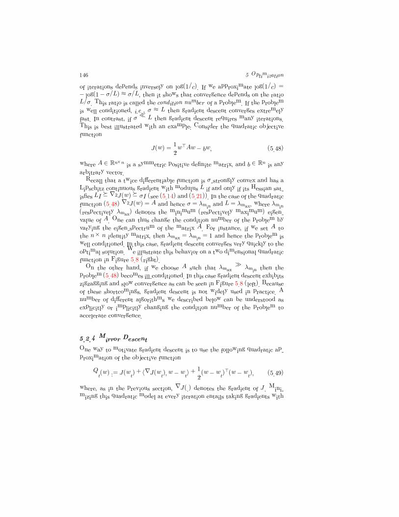
fast. In contrast, if σ � L then gradient descent requires many iterations.
This is best illustrated with an example: Consider the quadratic objective
function
J(w) =1
2w�Aw − bw� (5.48)
where A ∈ Rn×n is a symmetric positive definite matrix, and b ∈ R
n is any
arbitrary vector.
Recall that a twice differentiable function is σ-strongly convex and has a
Lipschitz continuous gradient with modulus L if and only if its Hessian sat-
isfies LI � ∇2J(w) � σI (see (5.14) and (5.21)). In the case of the quadratic
function (5.48) ∇2J(w) = A and hence σ = λmin and L = λmax, where λmin(respectively λmax) denotes the minimum (respectively maximum) eigen-
value of A. One can thus change the condition number of the problem by
varying the eigen-spectrum of the matrix A. For instance, if we set A to
the n × n identity matrix, then λmax = λmin = 1 and hence the problem is
well conditioned. In this case, gradient descent converges very quickly to the
optimal solution. We illustrate this behavior on a two dimensional quadratic
function in Figure 5.8 (right).
On the other hand, if we choose A such that λmax � λmin then the
problem (5.48) becomes ill-conditioned. In this case gradient descent exhibits
zigzagging and slow convergence as can be seen in Figure 5.8 (left). Because
of these shortcomings, gradient descent is not widely used in practice. A
number of different algorithms we described below can be understood as
explicitly or implicitly changing the condition number of the problem to
accelerate convergence.
5.2.4 Mirror Descent
One way to motivate gradient descent is to use the following quadratic ap-
proximation of the objective function
Qt(w) := J(wt) + �∇J(wt)� w − wt�+1
2(w − wt)
�(w − wt)� (5.49)
where, as in the previous section, ∇J(·) denotes the gradient of J . Mini-
mizing this quadratic model at every iteration entails taking gradients with
5.2 Unconstrained Smooth Convex Minimization 147
Fig. 5.8. Convergence of gradient descent with exact line search on two quadraticproblems (5.48). The problem on the left is ill-conditioned, whereas the problemon the right is well-conditioned. We plot the contours of the objective function,and the steps taken by gradient descent. As can be seen gradient descent convergesfast on the well conditioned problem, while it zigzags and takes many iterations toconverge on the ill-conditioned problem.
respect to w and setting it to zero, which gives
w − wt := −∇J(wt). (5.50)
Performing a line search along the direction −∇J(wt) recovers the familiar
gradient descent update
wt+1 = wt − ηt∇J(wt). (5.51)
The closely related mirror descent method replaces the quadratic penalty
in (5.49) by a Bregman divergence defined by some convex function f to
yield
Qt(w) := J(wt) + �∇J(wt)� w − wt�+Δf (w�wt). (5.52)
Computing the gradient, setting it to zero, and using∇wΔf (w�wt) = ∇f(w)−
∇f(wt), the minimizer of the above model can be written as
∇f(w)−∇f(wt) = −∇J(wt). (5.53)
As before, by using a stepsize ηt the resulting updates can be written as
wt+1 = ∇f−1(∇f(wt)− ηt∇J(wt)). (5.54)
It is easy to verify that choosing f(·) = 12 �·�
2 recovers the usual gradient
descent updates. On the other hand if we choose f to be the un-normalized
entropy (5.30) then ∇f(·) = log · and therefore (5.54) specializes to
wt+1 = exp(log(wt)− ηt∇J(wt)) = wt exp(−ηt∇J(wt))� (5.55)
which is sometimes called the Exponentiated Gradient (EG) update.
148 5 Optimization
Theorem 5.14 Let J be a convex function and J(w∗) denote its minimum
value. The mirror descent updates (5.54) with a σ-strongly convex function
f satisfy
Δf (w∗� w1) +
12σ
�t η
2t �∇J(wt)�
2
�t ηt
≥ mint
J(wt)− J(w∗).
Proof Using the convexity of J (see (5.7)) and (5.54) we can write
J(w∗) ≥ J(wt) + �w∗ − wt�∇J(wt)�
≥ J(wt)−1
ηt�w∗ − wt� f(wt+1)− f(wt)� .
Now applying Lemma 5.11 and rearranging
Δf (w∗� wt)−Δf (w
∗� wt+1) + Δf (wt� wt+1) ≥ ηt(J(wt)− J(w∗)).
Summing over t = 1� . . . � T
Δf (w∗� w1)−Δf (w
∗� wT+1) +�
t
Δf (wt� wt+1) ≥�
t
ηt(J(wt)− J(w∗)).
Noting that Δf (w∗� wT+1) ≥ 0, J(wt) − J(w∗) ≥ mint J(wt) − J(w∗), and
rearranging it follows that
Δf (w∗� w1) +
�tΔf (wt� wt+1)�
t ηt≥ min
tJ(wt)− J(w∗). (5.56)
Using (5.17) and (5.54)
Δf (wt� wt+1) ≤1
2σ�∇f(wt)−∇f(wt+1)�
2 =1
2ση2t �∇J(wt)�
2 . (5.57)
The proof is completed by plugging in (5.57) into (5.56).
Corollary 5.15 If J has a Lipschitz continuous gradient with modulus L,
and the stepsizes ηt are chosen as
ηt =
�2σΔf (w∗� w1)
L
1√tthen (5.58)
min1≤t≤T
J(wt)− J(w∗) ≤ L
�2Δf (w∗� w1)
σ
1√T.
Proof Since ∇J is Lipschitz continuous
min1≤t≤T
J(wt)− J(w∗) ≤Δf (w
∗� w1) +12σ
�t η
2tL
2
�t ηt
.
5.2 Unconstrained Smooth Convex Minimization 149
Plugging in (5.58) and using Problem 5.15
min1≤t≤T
J(wt)− J(w∗) ≤ L
�Δf (w∗� w1)
2σ
(1 +�
t1t )�
t1√t
≤ L
�Δf (w∗� w1)
2σ
1√T.
5.2.5 Conjugate Gradient
Let us revisit the problem of minimizing the quadratic objective function
(5.48). Since ∇J(w) = Aw− b, at the optimum ∇J(w) = 0 (see Lemma 5.6)
and hence
Aw = b. (5.59)
In fact, the Conjugate Gradient (CG) algorithm was first developed as a
method to solve the above linear system.
As we already saw, updating w along the negative gradient direction may
lead to zigzagging. Therefore CG uses the so-called conjugate directions.
Definition 5.16 �Conjugate Directions) Non zero vectors pt and pt� are
said to be conjugate with respect to a symmetric positive definite matrix A
if p�t�Apt = 0 if t �= t�.
Conjugate directions {p0� . . . � pn−1} are linearly independent and form a
basis. To see this, suppose the pt’s are not linearly independent. Then there
exists non-zero coefficients σt such that�
t σtpt = 0. The pt’s are conjugate
directions, therefore p�t�A(�
t σtpt) =�
t σtp�t�Apt = σt�p
�t�Apt� = 0 for all t�.
Since A is positive definite this implies that σt� = 0 for all t�, a contradiction.
As it turns out, the conjugate directions can be generated iteratively as
follows: Starting with any w0 ∈ Rn define p0 = −g0 = b−Aw0, and set
αt = −g�t pt
p�t Apt(5.60a)
wt+1 = wt + αtpt (5.60b)
gt+1 = Awt+1 − b (5.60c)
βt+1 =g�t+1Apt
p�t Apt(5.60d)
pt+1 = −gt+1 + βt+1pt (5.60e)
150 5 Optimization
The following theorem asserts that the pt generated by the above procedure
are indeed conjugate directions.
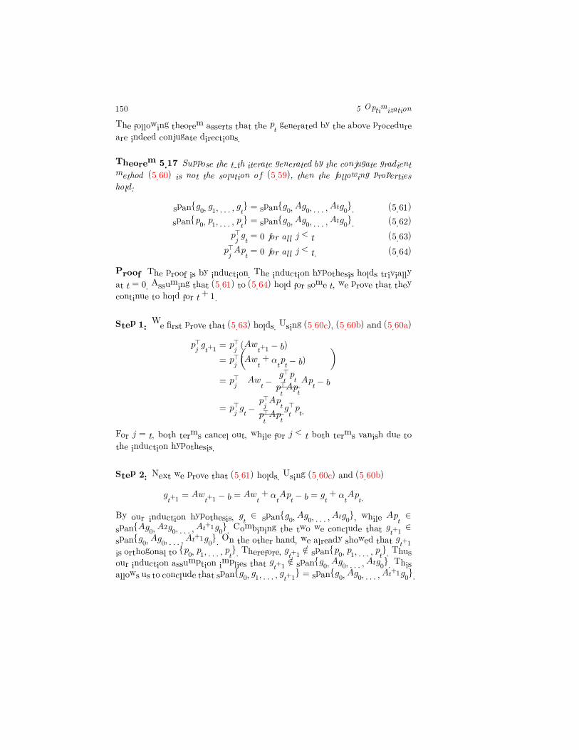
Theorem 5.17 Suppose the t-th iterate generated by the conjugate gradient
method (5.60) is not the solution of (5.59), then the following properties
hold:
span{g0� g1� . . . � gt} = span{g0� Ag0� . . . � Atg0}. (5.61)
span{p0� p1� . . . � pt} = span{g0� Ag0� . . . � Atg0}. (5.62)
p�j gt = 0 for all j < t (5.63)
p�j Apt = 0 for all j < t. (5.64)
Proof The proof is by induction. The induction hypothesis holds trivially
at t = 0. Assuming that (5.61) to (5.64) hold for some t, we prove that they
continue to hold for t+ 1.
Step 1: We first prove that (5.63) holds. Using (5.60c), (5.60b) and (5.60a)
p�j gt+1 = p�j (Awt+1 − b)
= p�j (Awt + αtpt − b)
= p�j
�
Awt −g�t pt
p�t AptApt − b
�
= p�j gt −p�j Apt
p�t Aptg�t pt.
For j = t, both terms cancel out, while for j < t both terms vanish due to
the induction hypothesis.
Step 2: Next we prove that (5.61) holds. Using (5.60c) and (5.60b)
gt+1 = Awt+1 − b = Awt + αtApt − b = gt + αtApt.
By our induction hypothesis, gt ∈ span{g0� Ag0� . . . � Atg0}, while Apt ∈
span{Ag0� A2g0� . . . � A
t+1g0}. Combining the two we conclude that gt+1 ∈
span{g0� Ag0� . . . � At+1g0}. On the other hand, we already showed that gt+1
is orthogonal to {p0� p1� . . . � pt}. Therefore, gt+1 /∈ span{p0� p1� . . . � pt}. Thus
our induction assumption implies that gt+1 /∈ span{g0� Ag0� . . . � Atg0}. This
allows us to conclude that span{g0� g1� . . . � gt+1} = span{g0� Ag0� . . . � At+1g0}.
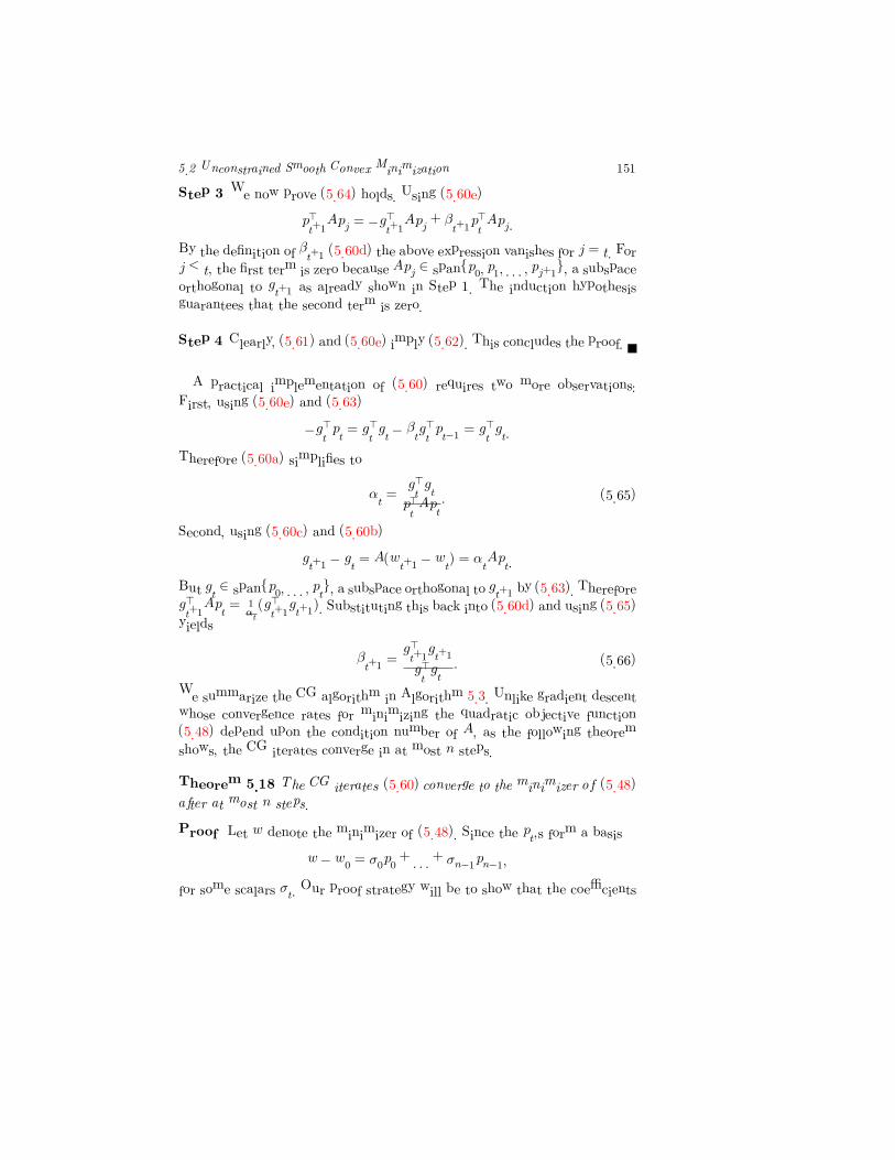
5.2 Unconstrained Smooth Convex Minimization 151
Step 3 We now prove (5.64) holds. Using (5.60e)
p�t+1Apj = −g�t+1Apj + βt+1p�t Apj .
By the definition of βt+1 (5.60d) the above expression vanishes for j = t. For
j < t, the first term is zero because Apj ∈ span{p0� p1� . . . � pj+1}, a subspace
orthogonal to gt+1 as already shown in Step 1. The induction hypothesis
guarantees that the second term is zero.
Step 4 Clearly, (5.61) and (5.60e) imply (5.62). This concludes the proof.
A practical implementation of (5.60) requires two more observations:
First, using (5.60e) and (5.63)
−g�t pt = g�t gt − βtg�t pt−1 = g�t gt.
Therefore (5.60a) simplifies to
αt =g�t gt
p�t Apt. (5.65)
Second, using (5.60c) and (5.60b)
gt+1 − gt = A(wt+1 − wt) = αtApt.
But gt ∈ span{p0� . . . � pt}, a subspace orthogonal to gt+1 by (5.63). Therefore
g�t+1Apt =1αt(g�t+1gt+1). Substituting this back into (5.60d) and using (5.65)
yields
βt+1 =g�t+1gt+1
g�t gt. (5.66)
We summarize the CG algorithm in Algorithm 5.3. Unlike gradient descent
whose convergence rates for minimizing the quadratic objective function
(5.48) depend upon the condition number of A, as the following theorem
shows, the CG iterates converge in at most n steps.
Theorem 5.18 The CG iterates (5.60) converge to the minimizer of (5.48)
after at most n steps.
Proof Let w denote the minimizer of (5.48). Since the pt’s form a basis
w − w0 = σ0p0 + . . .+ σn−1pn−1�
for some scalars σt. Our proof strategy will be to show that the coefficients
152 5 Optimization
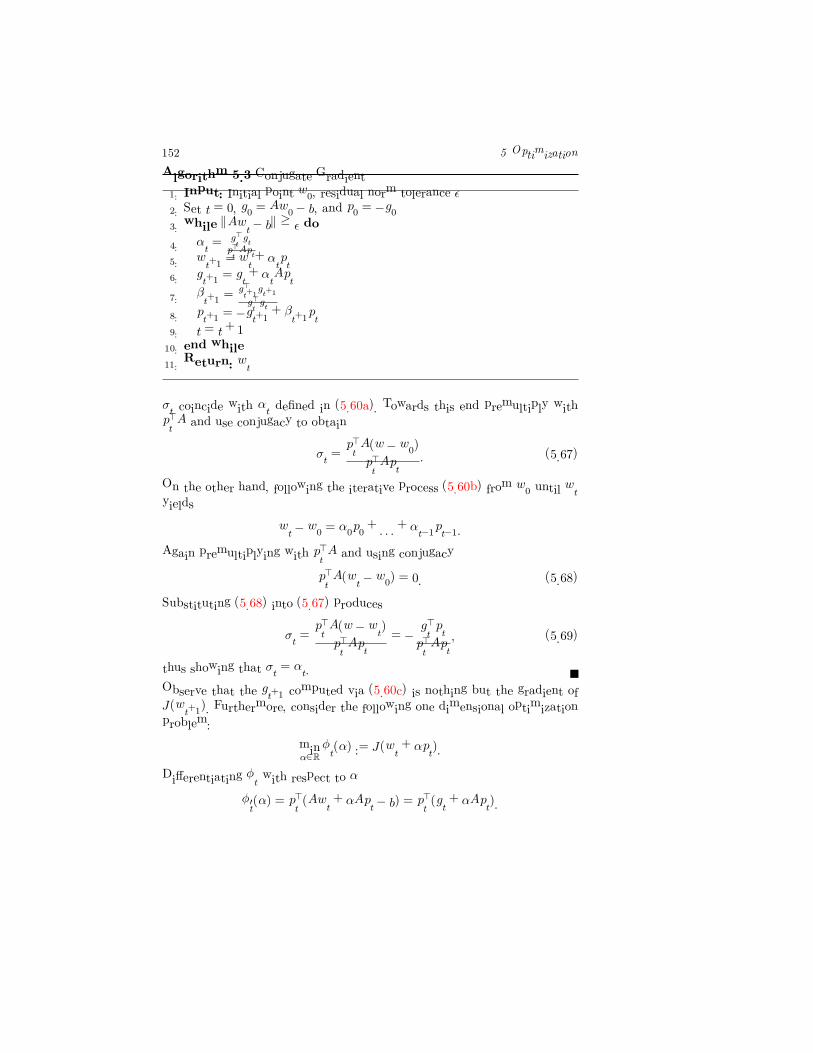
Algorithm 5.3 Conjugate Gradient
1: Input: Initial point w0, residual norm tolerance �
2: Set t = 0, g0 = Aw0 − b, and p0 = −g03: while �Awt − b� ≥ � do
4: αt =g�
tgt
p�tApt
5: wt+1 = wt + αtpt6: gt+1 = gt + αtApt
7: βt+1 =g�
t�1gt�1
g�tgt
8: pt+1 = −gt+1 + βt+1pt9: t = t+ 1
10: end while
11: Return: wt
σt coincide with αt defined in (5.60a). Towards this end premultiply with
p�t A and use conjugacy to obtain
σt =p�t A(w − w0)
p�t Apt. (5.67)
On the other hand, following the iterative process (5.60b) from w0 until wt
yields
wt − w0 = α0p0 + . . .+ αt−1pt−1.
Again premultiplying with p�t A and using conjugacy
p�t A(wt − w0) = 0. (5.68)
Substituting (5.68) into (5.67) produces
σt =p�t A(w − wt)
p�t Apt= −
g�t pt
p�t Apt� (5.69)
thus showing that σt = αt.
Observe that the gt+1 computed via (5.60c) is nothing but the gradient of
J(wt+1). Furthermore, consider the following one dimensional optimization
problem:
minα∈�
φt(α) := J(wt + αpt).
Differentiating φt with respect to α
φ�t(α) = p�t (Awt + αApt − b) = p�t (gt + αApt).
5.2 Unconstrained Smooth Convex Minimization 153
The gradient vanishes if we set α = −g�
tpt
p�tApt
, which recovers (5.60a). In other
words, every iteration of CG minimizes J(w) along a conjugate direction pt.
Contrast this with gradient descent which minimizes J(w) along the negative
gradient direction gt at every iteration.
It is natural to ask if this idea of generating conjugate directions and
minimizing the objective function along these directions can be applied to
general convex functions. The main difficulty here is that Theorems 5.17 and
5.18 do not hold. In spite of this, extensions of CG are effective even in this
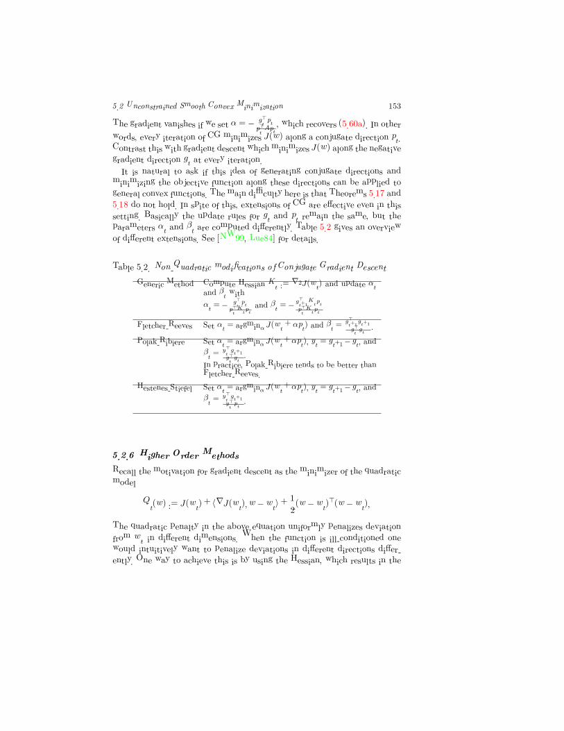
setting. Basically the update rules for gt and pt remain the same, but the
parameters αt and βt are computed differently. Table 5.2 gives an overview
of different extensions. See [NW99, Lue84] for details.
Table 5.2. Non-Quadratic modifications of Conjugate Gradient Descent
Generic Method Compute Hessian Kt := ∇2J(wt) and update αt
and βt with
αt = −g�
tpt
p�t
Ktpt
and βt = −g�
t�1Ktpt
p�t
Ktpt
Fletcher-Reeves Set αt = argminα J(wt + αpt) and βt =g�
t�1gt�1
g�t
gt
.
Polak-Ribiere Set αt = argminα J(wt +αpt), yt = gt�1− gt, and
βt =y�
tgt�1
g�t
gt
.
In practice, Polak-Ribiere tends to be better thanFletcher-Reeves.
Hestenes-Stiefel Set αt = argminα J(wt +αpt), yt = gt�1− gt, and
βt =y�
tgt�1
y�t
pt
.
5.2.6 Higher Order Methods
Recall the motivation for gradient descent as the minimizer of the quadratic
model
Qt(w) := J(wt) + �∇J(wt)� w − wt�+1
2(w − wt)
�(w − wt)�
The quadratic penalty in the above equation uniformly penalizes deviation
from wt in different dimensions. When the function is ill-conditioned one
would intuitively want to penalize deviations in different directions differ-
ently. One way to achieve this is by using the Hessian, which results in the
154 5 Optimization
Algorithm 5.4 Newton’s Method
1: Input: Initial point w0, gradient norm tolerance �
2: Set t = 0
3: while �∇J(wt)� > � do
4: Compute pt := −∇2J(wt)−1∇J(wt)
5: Compute ηt = argminη J(wt + ηpt) e.g., via Algorithm 5.1.
6: wt+1 = wt + ηtpt7: t = t+ 1
8: end while
9: Return: wt
following second order Taylor approximation:
Qt(w) := J(wt) + �∇J(wt)� w − wt�+1
2(w − wt)
�∇2J(wt)(w − wt).
(5.70)
Of course, this requires that J be twice differentiable. We will also assume
that J is strictly convex and hence its Hessian is positive definite and in-
vertible. Minimizing Qt by taking gradients with respect to w and setting it
zero obtains
w − wt := −∇2J(wt)−1∇J(wt)� (5.71)
Since we are only minimizing a model of the objective function, we perform
a line search along the descent direction (5.71) to compute the stepsize ηt,
which yields the next iterate:
wt+1 = wt − ηt∇2J(wt)
−1∇J(wt). (5.72)
Details can be found in Algorithm 5.4.
Suppose w∗ denotes the minimum of J(w). We say that an algorithm
exhibits quadratic convergence if the sequences of iterates {wk} generated
by the algorithm satisfies:
�wk+1 − w∗� ≤ C �wk − w∗�2 (5.73)
for some constant C > 0. We now show that Newton’s method exhibits
quadratic convergence close to the optimum.
Theorem 5.19 �Quadratic convergence of Newton’s Method) Suppose
J is twice differentiable, strongly convex, and the Hessian of J is bounded
and Lipschitz continuous with modulus M in a neighborhood of the so-
lution w∗. Furthermore, assume that��∇2J(w)−1
�� ≤ N . The iterations
5.2 Unconstrained Smooth Convex Minimization 155
wt+1 = wt−∇2J(wt)
−1∇J(wt) converge quadratically to w∗, the minimizer
of J .
Proof First notice that
∇J(wt)−∇J(w∗) =
� 1
0∇2J(wt + t(w∗ − wt))(wt − w∗)dt. (5.74)
Next using the fact that ∇2J(wt) is invertible and the gradient vanishes at
the optimum (∇J(w∗) = 0), write
wt+1 − w∗ = wt − w∗ −∇2J(wt)−1∇J(wt)
= ∇2J(wt)−1[∇2J(wt)(wt − w∗)− (∇J(wt)−∇J(w∗))]. (5.75)
Using (5.75), (5.74), and the Lipschitz continuity of ∇2J��∇J(wt)−∇J(w∗)−∇2J(wt)(wt − w∗)
��
=
����
� 1
0[∇2J(wt + t(wt − w∗))−∇2J(wt)](wt − w∗)dt
����
≤
� 1
0
��[∇2J(wt + t(wt − w∗))−∇2J(wt)]
�� �(wt − w∗)� dt
≤ �wt − w∗�2� 1
0Mtdt =
M
2�wt − w∗�2 . (5.76)
Finally use (5.75) and (5.76) to conclude that
�wt+1 − w∗� ≤M
2
��∇2J(wt)
−1�� �wt − w∗�2 ≤
NM
2�wt − w∗�2.
Newton’s method as we described it suffers from two major problems.
First, it applies only to twice differentiable, strictly convex functions. Sec-
ond, it involves computing and inverting of the n × n Hessian matrix at
every iteration, thus making it computationally very expensive. Although
Newton’s method can be extended to deal with positive semi-definite Hes-
sian matrices, the computational burden often makes it unsuitable for large
scale applications. In such cases one resorts to Quasi-Newton methods.
5.2.6.1 Quasi-Newton Methods
Unlike Newton’s method, which computes the Hessian of the objective func-
tion at every iteration, quasi-Newton methods never compute the Hessian;
they approximate it from past gradients. Since they do not require the ob-
jective function to be twice differentiable, quasi-Newton methods are much
156 5 Optimization
� � � � � � ����
���
�
���
���
���
���
����
����
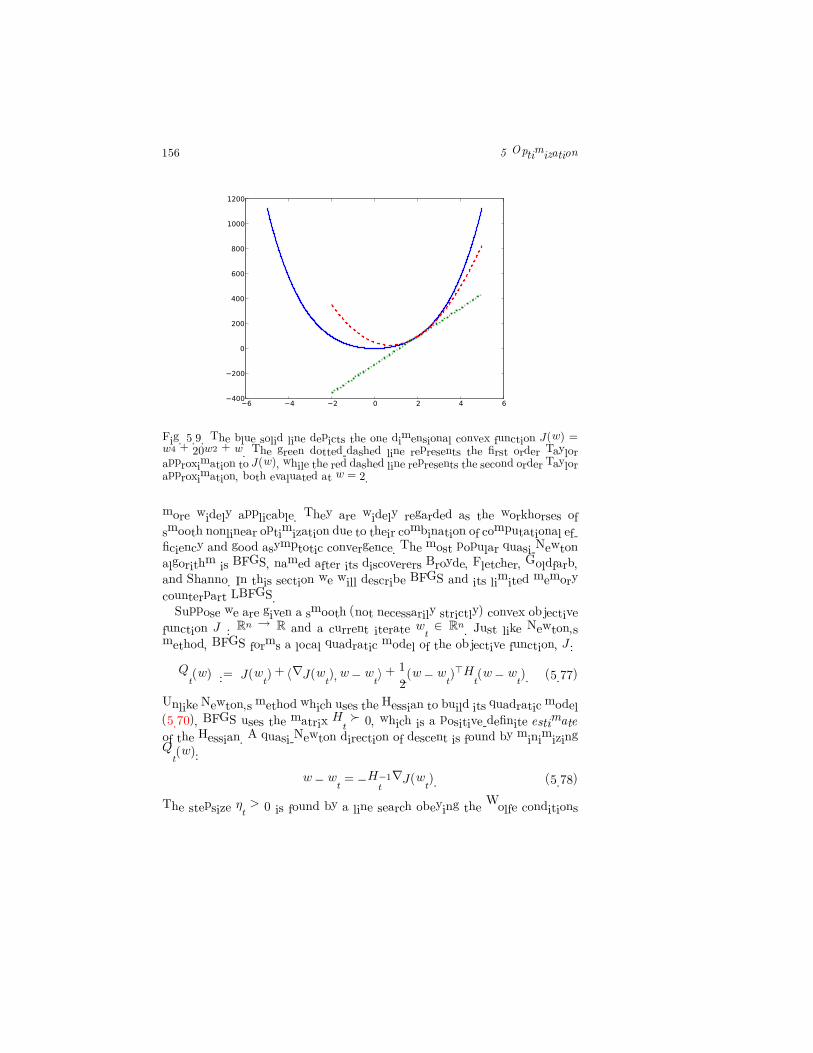
Fig. 5.9. The blue solid line depicts the one dimensional convex function J(w) =w4 + 20w2 + w. The green dotted-dashed line represents the first order Taylorapproximation to J(w), while the red dashed line represents the second order Taylorapproximation, both evaluated at w = 2.
more widely applicable. They are widely regarded as the workhorses of
smooth nonlinear optimization due to their combination of computational ef-
ficiency and good asymptotic convergence. The most popular quasi-Newton
algorithm is BFGS, named after its discoverers Broyde, Fletcher, Goldfarb,
and Shanno. In this section we will describe BFGS and its limited memory
counterpart LBFGS.
Suppose we are given a smooth (not necessarily strictly) convex objective
function J : Rn → R and a current iterate wt ∈ R
n. Just like Newton’s
method, BFGS forms a local quadratic model of the objective function, J :
Qt(w) := J(wt) + �∇J(wt)� w − wt�+1
2(w − wt)
�Ht(w − wt). (5.77)
Unlike Newton’s method which uses the Hessian to build its quadratic model
(5.70), BFGS uses the matrix Ht � 0, which is a positive-definite estimate
of the Hessian. A quasi-Newton direction of descent is found by minimizing
Qt(w):
w − wt = −H−1t ∇J(wt). (5.78)
The stepsize ηt > 0 is found by a line search obeying the Wolfe conditions
5.2 Unconstrained Smooth Convex Minimization 157
(5.42) and (5.43). The final update is given by
wt+1 = wt − ηtH−1t ∇J(wt). (5.79)
Given wt+1 we need to update our quadratic model (5.77) to
Qt+1(w) := J(wt+1) + �∇J(wt+1)� w − wt+1�+1
2(w − wt+1)
�Ht+1(w − wt+1).
(5.80)
When updating our model it is reasonable to expect that the gradient of
Qt+1 should match the gradient of J at wt and wt+1. Clearly,
∇Qt+1(w) = ∇J(wt+1) +Ht+1(w − wt+1)� (5.81)
which implies that ∇Qt+1(wt+1) = ∇J(wt+1), and hence our second con-
dition is automatically satisfied. In order to satisfy our first condition, we
require
∇Qt+1(wt) = ∇J(wt+1) +Ht+1(wt − wt+1) = ∇J(wt). (5.82)
By rearranging, we obtain the so-called secant equation:
Ht+1st = yt� (5.83)
where st := wt+1−wt and yt := ∇J(wt+1)−∇J(wt) denote the most recent
step along the optimization trajectory in parameter and gradient space,
respectively. Since Ht+1 is a positive definite matrix, pre-multiplying the
secant equation by st yields the curvature condition
s�t yt > 0. (5.84)
If the curvature condition is satisfied, then there are an infinite number
of matrices Ht+1 which satisfy the secant equation (the secant equation
represents n linear equations, but the symmetric matrix Ht+1 has n(n+1)/2
degrees of freedom). To resolve this issue we choose the closest matrix to
Ht which satisfies the secant equation. The key insight of the BFGS comes
from the observation that the descent direction computation (5.78) involves
the inverse matrix Bt := H−1t . Therefore, we choose a matrix Bt+1 := H−1
t+1
such that it is close to Bt and also satisfies the secant equation:
minB�B −Bt� (5.85)
s. t. B = B� and Byt = st. (5.86)
If the matrix norm �·� is appropriately chosen [NW99], then it can be shown
that
Bt+1 = (1−ρtsty�t )Bt(1−ρtyts
�t ) + ρtsts
�t � (5.87)
158 5 Optimization
Algorithm 5.5 LBFGS
1: Input: Initial point w0, gradient norm tolerance � > 0
2: Set t = 0 and B0 = I
3: while �∇J(wt)� > � do
4: pt = −Bt∇J(wt)
5: Find ηt that obeys (5.42) and (5.43)
6: st = ηtpt7: wt+1 = wt + st8: yt := ∇J(wt+1)−∇J(wt)
9: if t = 0 : Bt :=s�tyt
y�tyt
I
10: ρt = (s�t yt)−1
11: Bt+1 = (I − ρtsty�t )Bt(I − ρtyts
�t ) + ρtsts
�t
12: t = t+ 1
13: end while
14: Return: wt
where ρt := (y�t st)−1. In other words, the matrix Bt is modified via an
incremental rank-two update, which is very efficient to compute, to obtain
Bt+1.
There exists an interesting connection between the BFGS update (5.87)
and the Hestenes-Stiefel variant of Conjugate gradient. To see this assume
that an exact line search was used to compute wt+1, and therefore s�t ∇J(wt+1) =
0. Furthermore, assume that Bt = 1, and use (5.87) to write
pt+1 = −Bt+1∇J(wt+1) = −∇J(wt+1) +y�t ∇J(wt+1)
y�t stst� (5.88)
which recovers the Hestenes-Stiefel update (see (5.60e) and Table 5.2).
Limited-memory BFGS (LBFGS) is a variant of BFGS designed for solv-
ing large-scale optimization problems where the O(d2) cost of storing and
updating Bt would be prohibitively expensive. LBFGS approximates the
quasi-Newton direction (5.78) directly from the last m pairs of st and yt via
a matrix-free approach. This reduces the cost to O(md) space and time per
iteration, with m freely chosen. Details can be found in Algorithm 5.5.
5.2.6.2 Spectral Gradient Methods
Although spectral gradient methods do not use the Hessian explicitly, they
are motivated by arguments very reminiscent of the Quasi-Newton methods.
Recall the update rule (5.79) and secant equation (5.83). Suppose we want
5.2 Unconstrained Smooth Convex Minimization 159
a very simple matrix which approximates the Hessian. Specifically, we want
Ht+1 = αt+1I (5.89)
where αt+1 is a scalar and I denotes the identity matrix. Then the secant
equation (5.83) becomes
αt+1st = yt. (5.90)
In general, the above equation cannot be solved. Therefore we use the αt+1
which minimizes �αt+1st − yt�2 which yields the Barzilai-Borwein (BB) step-
size
αt+1 =s�t yt
s�t st. (5.91)
As it turns out, αt+1 lies between the minimum and maximum eigenvalue of
the average Hessian in the direction st, hence the name Spectral Gradient
method. The parameter update (5.79) is now given by
wt+1 = wt −1
αt∇J(wt). (5.92)
A practical implementation uses safeguards to ensure that the stepsize αt+1
is neither too small nor too large. Given 0 < αmin < αmax <∞ we compute
αt+1 = min
�
αmax�max
�
αmin�s�t yt
s�t st
��
. (5.93)
One of the peculiar features of spectral gradient methods is their use
of a non-monotone line search. In all the algorithms we have seen so far,
the stepsize is chosen such that the objective function J decreases at every
iteration. In contrast, non-monotone line searches employ a parameter M ≥
1 and ensure that the objective function decreases in every M iterations. Of
course, setting M = 1 results in the usual monotone line search. Details can
be found in Algorithm 5.6.
5.2.7 Bundle Methods
The methods we discussed above are applicable for minimizing smooth, con-
vex objective functions. Some regularized risk minimization problems involve
a non-smooth objective function. In such cases, one needs to use bundle
methods. In order to lay the ground for bundle methods we first describe
their precursor the cutting plane method [Kel60]. Cutting plane method is
based on a simple observation: A convex function is bounded from below by
160 5 Optimization
Algorithm 5.6 Spectral Gradient Method
1: Input: w0, M ≥ 1, αmax > αmin > 0, γ ∈ (0� 1), 1 > σ2 > σ1 > 0,
α0 ∈ [αmin� αmax], and � > 0
2: Initialize: t = 0
3: while �∇J(wt)� > � do
4: λ = 1
5: while TRUE do
6: dt = − 1αt∇J(wt)
7: w+ = wt + λdt8: δ = �dt�∇J(wt)�
9: if J(w+) ≤ min0≤j≤min(t�M−1) J(xt−j) + γλδ then
10: wt+1 = w+
11: st = wt+1 − wt
12: yt = ∇J(wt+1)−∇J(wt)
13: break
14: else
15: λtmp = −12λ
2δ/(J(w+ − J(wt)− λδ)
16: if λtmp > σ1 and λtmp < σ2λ then
17: λ = λtmp
18: else
19: λ = λ/2
20: end if
21: end if
22: end while
23: αt+1 = min(αmax�max(αmin�s�tyt
s�tst
))
24: t = t+ 1
25: end while
26: Return: wt
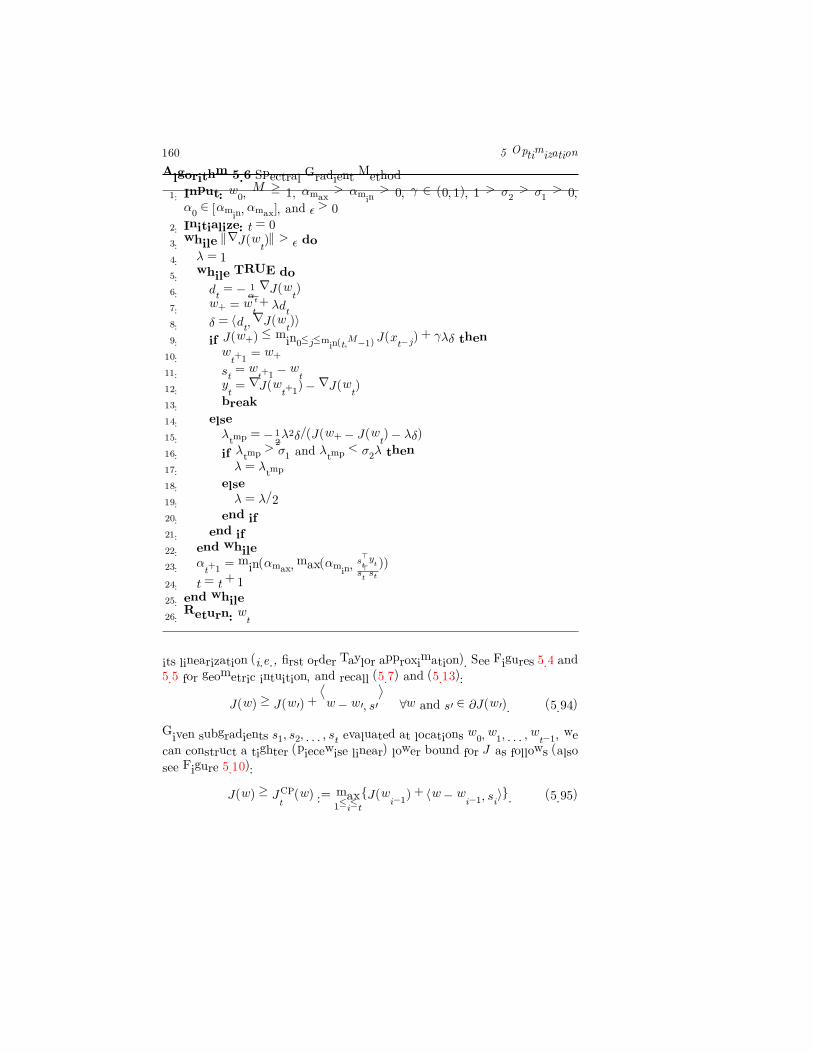
its linearization (i.e., first order Taylor approximation). See Figures 5.4 and
5.5 for geometric intuition, and recall (5.7) and (5.13):
J(w) ≥ J(w�) +�w − w�� s�
�∀w and s� ∈ ∂J(w�). (5.94)
Given subgradients s1� s2� . . . � st evaluated at locations w0� w1� . . . � wt−1, we
can construct a tighter (piecewise linear) lower bound for J as follows (also
see Figure 5.10):
J(w) ≥ JCPt (w) := max1≤i≤t
{J(wi−1) + �w − wi−1� si�}. (5.95)
5.2 Unconstrained Smooth Convex Minimization 161
Given iterates {wi}t−1i=0, the cutting plane method minimizes JCPt to obtain
the next iterate wt:
wt := argminw
JCPt (w). (5.96)
This iteratively refines the piecewise linear lower bound JCP and allows us
to get close to the minimum of J (see Figure 5.10 for an illustration).
If w∗ denotes the minimizer of J , then clearly each J(wi) ≥ J(w∗) and
hence min0≤i≤t J(wi) ≥ J(w∗). On the other hand, since J ≥ JCPt it fol-
lows that J(w∗) ≥ JCPt (wt). In other words, J(w∗) is sandwiched between
min0≤i≤t J(wi) and JCPt (wt) (see Figure 5.11 for an illustration). The cutting
plane method monitors the monotonically decreasing quantity
�t := min0≤i≤t
J(wi)− JCPt (wt)� (5.97)
and terminates whenever �t falls below a predefined threshold �. This ensures
that the solution J(wt) is � optimum, that is, J(wt) ≤ J(w∗) + �.
Fig. 5.10. A convex function (blue solid curve) is bounded from below by its lin-earizations (dashed lines). The gray area indicates the piecewise linear lower boundobtained by using the linearizations. We depict a few iterations of the cutting planemethod. At each iteration the piecewise linear lower bound is minimized and a newlinearization is added at the minimizer (red rectangle). As can be seen, adding morelinearizations improves the lower bound.
Although cutting plane method was shown to be convergent [Kel60], it is
162 5 Optimization
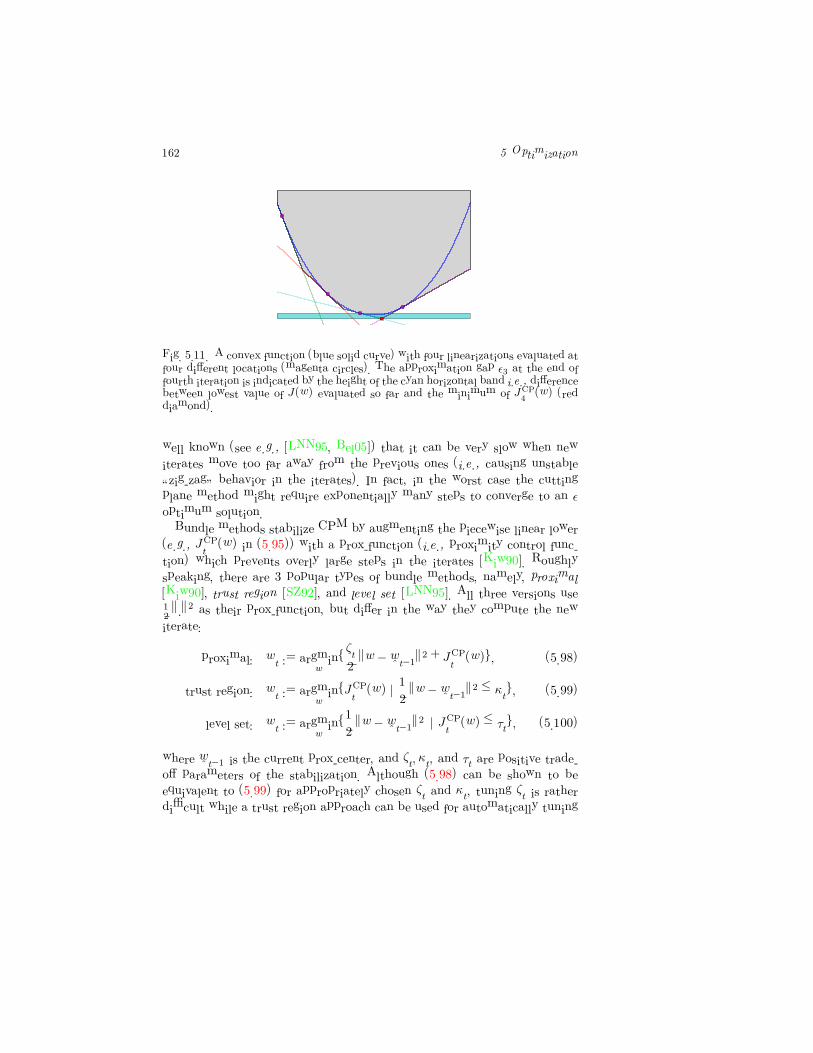
Fig. 5.11. A convex function (blue solid curve) with four linearizations evaluated atfour different locations (magenta circles). The approximation gap �3 at the end offourth iteration is indicated by the height of the cyan horizontal band i.e., differencebetween lowest value of J(w) evaluated so far and the minimum of JCP
4 (w) (reddiamond).
well known (see e.g., [LNN95, Bel05]) that it can be very slow when new
iterates move too far away from the previous ones (i.e., causing unstable
“zig-zag” behavior in the iterates). In fact, in the worst case the cutting
plane method might require exponentially many steps to converge to an �
optimum solution.
Bundle methods stabilize CPM by augmenting the piecewise linear lower
(e.g., JCPt (w) in (5.95)) with a prox-function (i.e., proximity control func-
tion) which prevents overly large steps in the iterates [Kiw90]. Roughly
speaking, there are 3 popular types of bundle methods, namely, proximal
[Kiw90], trust region [SZ92], and level set [LNN95]. All three versions use12 �·�
2 as their prox-function, but differ in the way they compute the new
iterate:
proximal: wt := argminw
{ζt2�w − wt−1�
2 + JCPt (w)}� (5.98)
trust region: wt := argminw
{JCPt (w) |1
2�w − wt−1�
2 ≤ κt}� (5.99)
level set: wt := argminw
{1
2�w − wt−1�
2 | JCPt (w) ≤ τt}� (5.100)
where wt−1 is the current prox-center, and ζt� κt� and τt are positive trade-
off parameters of the stabilization. Although (5.98) can be shown to be
equivalent to (5.99) for appropriately chosen ζt and κt, tuning ζt is rather
difficult while a trust region approach can be used for automatically tuning
5.3 Constrained Optimization 163
κt. Consequently the trust region algorithm BT of [SZ92] is widely used in
practice.
5.3 Constrained Optimization
So far our focus was on unconstrained optimization problems. Many ma-
chine learning problems involve constraints, and can often be written in the
following canonical form:
minw
J(w) (5.101a)
s. t. ci(w) ≤ 0 for i ∈ I (5.101b)
ei(w) = 0 for i ∈ E (5.101c)
where both ci and ei are convex functions. We say that w is feasible if and
only if it satisfies the constraints, that is, ci(w) ≤ 0 for i ∈ I and ei(w) = 0
for i ∈ E.
Recall that w is the minimizer of an unconstrained problem if and only if
�∇J(w)� = 0 (see Lemma 5.6). Unfortunately, when constraints are present
one cannot use this simple characterization of the solution. For instance, the
w at which �∇J(w)� = 0 may not be a feasible point. To illustrate, consider
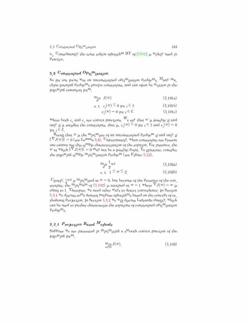
the following simple minimization problem (see Figure 5.12):
minw
1
2w2 (5.102a)
s. t. 1 ≤ w ≤ 2. (5.102b)
Clearly, 12w
2 is minimized at w = 0, but because of the presence of the con-
straints, the minimum of (5.102) is attained at w = 1 where ∇J(w) = w is
equal to 1. Therefore, we need other ways to detect convergence. In Section
5.3.1 we discuss some general purpose algorithms based on the concept of or-
thogonal projection. In Section 5.3.2 we will discuss Lagrange duality, which
can be used to further characterize the solutions of constrained optimization
problems.
5.3.1 Projection Based Methods
Suppose we are interested in minimizing a smooth convex function of the
following form:
minw∈Ω
J(w)� (5.103)
164 5 Optimization
� � � � � � ��
�
�
�
�
�
��
��
��
����
Fig. 5.12. The unconstrained minimum of the quadratic function 1
2w2 is attained
at w = 0 (red circle). But, if we enforce the constraints 1 ≤ w ≤ 2 (illustrated bythe shaded area) then the minimizer is attained at w = 1 (green diamond).
where Ω is a convex feasible region. For instance, Ω may be described by
convex functions ci and ei as in (5.101). The algorithms we describe in this
section are applicable when Ω is a relatively simple set onto which we can
compute an orthogonal projection. Given a point w� and a feasible region
Ω, the orthogonal projection PΩ(w�) of w� on Ω is defined as
PΩ(w�) := argmin
w∈Ω
��w� − w
��2 . (5.104)
Geometrically speaking, PΩ(w�) is the closest point to w� in Ω. Of course, if
w� ∈ Ω then PΩ(w�) = w�.
We are interested in finding an approximate solution of (5.103), that is,
a w ∈ Ω such that
J(w)−minw∈Ω
J(w) = J(w)− J∗ ≤ �� (5.105)
for some pre-defined tolerance � > 0. Of course, J∗ is unknown and hence the
gap J(w)− J∗ cannot be computed in practice. Furthermore, as we showed
in Section 5.3, for constrained optimization problems �∇J(w)� does not
vanish at the optimal solution. Therefore, we will use the following stopping
5.3 Constrained Optimization 165
Algorithm 5.7 Basic Projection Based Method
1: Input: Initial point w0 ∈ Ω, and projected gradient norm tolerance
� > 0
2: Initialize: t = 0
3: while �PΩ(wt −∇J(wt))− wt� > � do
4: Find direction of descent dt5: wt+1 = PΩ(wt + ηtdt)
6: t = t+ 1
7: end while
8: Return: wt
criterion in our algorithms
�PΩ(wt −∇J(wt))− wt� ≤ �. (5.106)
The intuition here is as follows: If wt − ∇J(wt) ∈ Ω then PΩ(wt −
∇J(wt)) = wt if, and only if, ∇J(wt) = 0, that is, wt is the global minimizer
of J(w). On the other hand, if wt−∇J(wt) /∈ Ω but PΩ(wt−∇J(wt)) = wt,
then the constraints are preventing us from making any further progress
along the descent direction −∇J(wt) and hence we should stop.
The basic projection based method is described in Algorithm 5.7. Any
unconstrained optimization algorithm can be used to generate the direction
of descent dt. A line search is used to find the stepsize ηt. The updated
parameter wt − ηtdt is projected onto Ω to obtain wt+1. If dt is chosen to
be the negative gradient direction −∇J(wt), then the resulting algorithm
is called the projected gradient method. One can show that the rates of
convergence of gradient descent with various line search schemes is also
preserved by projected gradient descent.
5.3.2 Lagrange Duality
Lagrange duality plays a central role in constrained convex optimization.
The basic idea here is to augment the objective function (5.101) with a
weighted sum of the constraint functions by defining the Lagrangian:
L(w�α� β) = J(w) +�
i∈I
αici(w) +�
i∈E
βiei(w) (5.107)
for αi ≥ 0 and βi ∈ R. In the sequel, we will refer to α (respectively β) as the
Lagrange multipliers associated with the inequality (respectively equality)
constraints. Furthermore, we will call α and β dual feasible if and only if
166 5 Optimization
αi ≥ 0 and βi ∈ R. The Lagrangian satisfies the following fundamental
property, which makes it extremely useful for constrained optimization.
Theorem 5.20 The Lagrangian (5.107) of (5.101) satisfies
maxα≥0�β
L(w�α� β) =
�J(w) if w is feasible
∞ otherwise.
In particular, if J∗ denotes the optimal value of (5.101), then
J∗ = minw
maxα≥0�β
L(w�α� β).
Proof First assume that w is feasible, that is, ci(w) ≤ 0 for i ∈ I and
ei(w) = 0 for i ∈ E. Since αi ≥ 0 we have
�
i∈I
αici(w) +�
i∈E
βiei(w) ≤ 0� (5.108)
with equality being attained by setting αi = 0 whenever ci(w) < 0. Conse-
quently,
maxα≥0�β
L(w�α� β) = maxα≥0�β
J(w) +�
i∈I
αici(w) +�
i∈E
βiei(w) = J(w)
whenever w is feasible. On the other hand, if w is not feasible then either
ci�(w) > 0 or ei�(w) �= 0 for some i�. In the first case simply let αi� →∞ to
see that maxα≥0�β L(w�α� β) → ∞. Similarly, when ei�(w) �= 0 let βi� → ∞
if ei�(w) > 0 or βi� → −∞ if ei�(w) < 0 to arrive at the same conclusion.
If define the Lagrange dual function
D(α� β) = minw
L(w�α� β)� (5.109)
for α ≥ 0 and β, then one can prove the following property, which is often
called as weak duality.
Theorem 5.21 �Weak Duality) The Lagrange dual function (5.109) sat-
isfies
D(α� β) ≤ J(w)
for all feasible w and α ≥ 0 and β. In particular
D∗ := maxα≥0�β
minw
L(w�α� β) ≤ minw
maxα≥0�β
L(w�α� β) = J∗. (5.110)
5.3 Constrained Optimization 167
Proof As before, observe that whenever w is feasible�
i∈I
αici(w) +�
i∈E
βiei(w) ≤ 0.
Therefore
D(α� β) = minw
L(w�α� β) = minw
J(w) +�
i∈I
αici(w) +�
i∈E
βiei(w) ≤ J(w)
for all feasible w and α ≥ 0 and β. In particular, one can choose w to be
the minimizer of (5.101) and α ≥ 0 and β to be maximizers of D(α� β) to
obtain (5.110).
Weak duality holds for any arbitrary function, not-necessarily convex. When
the objective function and constraints are convex, and certain technical con-
ditions, also known as Slater’s conditions hold, then we can say more.
Theorem 5.22 �Strong Duality) Supposed the objective function f and
constraints ci for i ∈ I and ei for i ∈ E in (5.101) are convex and the
following constraint qualification holds:
There exists a w such that ci(w) < 0 for all i ∈ I.
Then the Lagrange dual function (5.109) satisfies
D∗ := maxα≥0�β
minw
L(w�α� β) = minw
maxα≥0�β
L(w�α� β) = J∗. (5.111)
The proof of the above theorem is quite technical and can be found in
any standard reference (e.g., [BV04]). Therefore we will omit the proof and
proceed to discuss various implications of strong duality. First note that
minw
maxα≥0�β
L(w�α� β) = maxα≥0�β
minw
L(w�α� β). (5.112)
In other words, one can switch the order of minimization over w with max-
imization over α and β. This is called the saddle point property of convex
functions.
Suppose strong duality holds. Given any α ≥ 0 and β such that D(α� β) >
−∞ and a feasible w we can immediately write the duality gap
J(w)− J∗ = J(w)−D∗ ≤ J(w)−D(α� β)�
where J∗ and D∗ were defined in (5.111). Below we show that if w∗ is primal
optimal and (α∗� β∗) are dual optimal then J(w∗) − D(α∗� β∗) = 0. This
provides a non-heuristic stopping criterion for constrained optimization: stop
when J(w)−D(α� β) ≤ �, where � is a pre-specified tolerance.
168 5 Optimization
Suppose the primal and dual optimal values are attained at w∗ and
(α∗� β∗) respectively, and consider the following line of argument:
J(w∗) = D(α∗� β∗) (5.113a)
= minw
J(w) +�
i∈I
α∗i ci(w) +�
i∈E
β∗i ej(w) (5.113b)
≤ J(w∗) +�
i∈I
α∗i ci(w∗) +
�
i∈E
β∗i ei(w∗) (5.113c)
≤ J(w∗). (5.113d)
To write (5.113a) we used strong duality, while (5.113c) obtains by setting
w = w∗ in (5.113c). Finally, to obtain (5.113d) we used the fact that w∗ is
feasible and hence (5.108) holds. Since (5.113) holds with equality, one can
conclude that the following complementary slackness condition:
�
i∈I
α∗i ci(w∗) +
�
i∈E
β∗i ei(w∗) = 0.
In other words, α∗i ci(w∗) = 0 or equivalently α∗i = 0 whenever ci(w) < 0.
Furthermore, since w∗ minimizes L(w�α∗� β∗) over w, it follows that its
gradient must vanish at w∗, that is,
∇J(w∗) +�
i∈I
α∗i∇ci(w∗) +
�
i∈E
β∗i∇ei(w∗) = 0.
Putting everything together, we obtain
ci(w∗) ≤ 0 ∀i ∈ I (5.114a)
ej(w∗) = 0 ∀i ∈ E (5.114b)
α∗i ≥ 0 (5.114c)
α∗i ci(w∗) = 0 (5.114d)
∇J(w∗) +�
i∈I
α∗i∇ci(w∗) +
�
i∈E
β∗i∇ei(w∗) = 0. (5.114e)
The above conditions are called the KKT conditions. If the primal problem is
convex, then the KKT conditions are both necessary and sufficient. In other
words, if w and (α� β) satisfy (5.114) then w and (α� β) are primal and dual
optimal with zero duality gap. To see this note that the first two conditions
show that w is feasible. Since αi ≥ 0, L(w�α� β) is convex in w. Finally the
last condition states that w minimizes L(w� α� β). Since αici(w) = 0 and
5.3 Constrained Optimization 169
ej(w) = 0, we have
D(α� β) = minw
L(w� α� β)
= J(w) +n�
i=1
αici(w) +m�
j=1
βjej(w)
= J(w).
5.3.3 Linear and Quadratic Programs
So far we discussed general constrained optimization problems. Many ma-
chine learning problems have special structure which can be exploited fur-
ther. We discuss the implication of duality for two such problems.
5.3.3.1 Linear Programming
An optimization problem with a linear objective function and (both equality
and inequality) linear constraints is said to be a linear program (LP). A
canonical linear program is of the following form:
minw
c�w (5.115a)
s. t. Aw = b� w ≥ 0. (5.115b)
Here w and c are n dimensional vectors, while b is a m dimensional vector,
and A is a m× n matrix with m < n.
Suppose we are given a LP of the form:
minw
c�w (5.116a)
s. t. Aw ≥ b� (5.116b)
we can transform it into a canonical LP by introducing non-negative slack
variables
minw�ξ
c�w (5.117a)
s. t. Aw − ξ = b� ξ ≥ 0. (5.117b)
Next, we split w into its positive and negative parts w+ and w− respec-
tively by setting w+i = max(0� wi) and w−i = max(0�−wi). Using these new
170 5 Optimization
variables we rewrite (5.117) as
minw��w�� ξ
c
−c
0
�
w+
w−
ξ
(5.118a)
s. t.�A −A −I
�
w+
w−
ξ
= b�
w+
w−
ξ
≥ 0� (5.118b)
thus yielding a canonical LP (5.115) in the variables w+, w− and ξ.
By introducing non-negative Lagrange multipliers α and β one can write
the Lagrangian of (5.115) as
L(w� β� s) = c�w + β�(Aw − b)− α�w. (5.119)
Taking gradients with respect to the primal and dual variables and setting
them to zero obtains
A�β − α = c (5.120a)
Aw = b (5.120b)
α�w = 0 (5.120c)
w ≥ 0 (5.120d)
α ≥ 0. (5.120e)
Condition (5.120c) can be simplified by noting that both w and α are con-
strained to be non-negative, therefore α�w = 0 if, and only if, αiwi = 0 for
i = 1� . . . � n.
Using (5.120a), (5.120c), and (5.120b) we can write
c�w = (A�β − α)�w = β�Aw = β�b.
Substituting this into (5.115) and eliminating the primal variable w yields
the following dual LP
maxα�β
b�β (5.121a)
s.t. A�β − α = c� α ≥ 0. (5.121b)
As before, we let β+ = max(β� 0) and β− = max(0�−β) and convert the
5.3 Constrained Optimization 171
above LP into the following canonical LP
maxα�β��β�
b
−b
0
�
β+
β−
α
(5.122a)
s.t.�A� −A� −I
�
β+
β−
α
= c�
β+
β−
α
≥ 0. (5.122b)
It can be easily verified that the primal-dual problem is symmetric; by taking
the dual of the dual we recover the primal (Problem 5.17). One important
thing to note however is that the primal (5.115) involves n variables and
n + m constraints, while the dual (5.122) involves 2m + n variables and
4m+ 2n constraints.
5.3.3.2 Quadratic Programming
An optimization problem with a convex quadratic objective function and lin-
ear constraints is said to be a convex quadratic program (QP). The canonical
convex QP can be written as follows:
minw
1
2w�Gx+ w�d (5.123a)
s.t. a�i w = bi for i ∈ E (5.123b)
a�i w ≤ bi for i ∈ I (5.123c)
Here G � 0 is a n× n positive semi-definite matrix, E and I are finite set of
indices, while d and ai are n dimensional vectors, and bi are scalars.
As a warm up let us consider the arguably simpler equality constrained
quadratic programs. In this case, we can stack the ai into a matrix A and
the bi into a vector b to write
minw
1
2w�Gw + w�d (5.124a)
s.t. Aw = b (5.124b)
By introducing non-negative Lagrange multipliers β the Lagrangian of the
above optimization problem can be written as
L(w� β) =1
2w�Gw + w�d+ β(Aw − b). (5.125)
To find the saddle point of the Lagrangian we take gradients with respect
172 5 Optimization
to w and β and set them to zero. This obtains
Gw + d+A�β = 0
Aw = b.
Putting these two conditions together yields the following linear system of
equations�G A�
A 0
� �w
β
�
=
�−d
b
�
. (5.126)
The matrix in the above equation is called the KKT matrix, and we can use
it to characterize the conditions under which (5.124) has a unique solution.
Theorem 5.23 Let Z be a n× (n−m) matrix whose columns form a basis
for the null space of A, that is, AZ = 0. If A has full row rank, and the
reduced-Hessian matrix Z�GZ is positive definite, then there exists a unique
pair (w∗� β∗) which solves (5.126). Furthermore, w∗ also minimizes (5.124).
Proof Note that a unique (w∗� β∗) exists whenever the KKT matrix is
non-singular. Suppose this is not the case, then there exist non-zero vectors
a and b such that�G A�
A 0
� �a
b
�
= 0.
Since Aa = 0 this implies that a lies in the null space of A and hence there
exists a u such that a = Zu. Therefore
�Zu 0
��G A�
A 0
� �Zu
0
�
= u�Z�GZu = 0.
Positive definiteness of Z�GZ implies that u = 0 and hence a = 0. On the
other hand, the full row rank of A and A�b = 0 implies that b = 0. In
summary, both a and b are zero, a contradiction.
Let w �= w∗ be any other feasible point and Δw = w∗ − w. Since Aw∗ =
Aw = b we have that AΔw = 0. Hence, there exists a non-zero u such that
Δw = Zu. The objective function J(w) can be written as
J(w) =1
2(w∗ −Δw)�G(w∗ −Δw) + (w∗ −Δw)�d
= J(w∗) +1
2Δw�GΔw − (Gw∗ + d)�Δw.
First note that 12Δw�GΔw = 1
2u�Z�GZu > 0 by positive definiteness of
the reduced Hessian. Second, since w∗ solves (5.126) it follows that (Gw∗ +
5.4 Stochastic Optimization 173
d)�Δw = β�AΔw = 0. Together these two observations imply that J(w) >
J(w∗).
If the technical conditions of the above theorem are met, then solving the
equality constrained QP (5.124) is equivalent to solving the linear system
(5.126). See [NW99] for a extensive discussion of algorithms that can be
used for this task.
Next we turn our attention to the general QP (5.123) which also contains
inequality constraints. The Lagrangian in this case can be written as
L(w� β) =1
2w�Gw + w�d+
�
i∈I
αi(a�i w − bi) +
�
i∈E
βi(a�i w − bi). (5.127)
Let w∗ denote the minimizer of (5.123). If we define the active set �(w∗) as
�(w∗) =�i s.t. i ∈ I and a�i w
∗ = bi
��
then the KKT conditions (5.114) for this problem can be written as
a�i w − bi < 0 ∀i ∈ I ��(w∗) (5.128a)
a�i w − bi = 0 ∀i ∈ E ∪�(w∗) (5.128b)
α∗i ≥ 0 ∀i ∈ �(w∗) (5.128c)
Gw∗ + d+�
i∈�(w∗)
α∗i ai +�
i∈E
βiai = 0. (5.128d)
Conceptually the main difficulty in solving (5.123) is in identifying the active
set �(w∗). This is because α∗i = 0 for all i ∈ I � �(w∗). Most algorithms
for solving (5.123) can be viewed as different ways to identify the active set.
See [NW99] for a detailed discussion.
5.4 Stochastic Optimization
Recall that regularized risk minimization involves a data-driven optimization
problem in which the objective function involves the summation of loss terms
over a set of data to be modeled:
minf
J(f) := λΩ(f) +1
m
m�
i=1
l(f(xi)� yi).
Classical optimization techniques must compute this sum in its entirety for
each evaluation of the objective, respectively its gradient. As available data
sets grow ever larger, such “batch” optimizers therefore become increasingly
inefficient. They are also ill-suited for the incremental setting, where partial
data must be modeled as it arrives.
174 5 Optimization
Stochastic gradient-based methods, by contrast, work with gradient esti-
mates obtained from small subsamples (mini-batches) of training data. This
can greatly reduce computational requirements: on large, redundant data
sets, simple stochastic gradient descent routinely outperforms sophisticated
second-order batch methods by orders of magnitude.
The key idea here is that J(w) is replaced by an instantaneous estimate
Jt which is computed from a mini-batch of size k comprising of a subset of
points (xti� yti) with i = 1� . . . � k drawn from the dataset:
Jt(w) = λΩ(w) +1
k
k�
i=1
l(w� xti� yti). (5.129)
Setting k = 1 obtains an algorithm which processes data points as they
arrive.
5.4.1 Stochastic Gradient Descent
Perhaps the simplest stochastic optimization algorithm is Stochastic Gradi-
ent Descent (SGD). The parameter update of SGD takes the form:
wt+1 = wt − ηt∇Jt(wt). (5.130)
If Jt is not differentiable, then one can choose an arbitrary subgradient from
∂Jt(wt) to compute the update. It has been shown that SGD asymptotically
converges to the true minimizer of J(w) if the stepsize ηt decays as O(1/√t).
For instance, one could set
ηt =
�τ
τ + t� (5.131)
where τ > 0 is a tuning parameter. See Algorithm 5.8 for details.
5.4.1.1 Practical Considerations
One simple yet effective rule of thumb to tune τ is to select a small subset
of data, try various values of τ on this subset, and choose the τ that most
reduces the objective function.
In some cases letting ηt to decay as O(1/t) has been found to be more
effective:
ηt =τ
τ + t. (5.132)
The free parameter τ > 0 can be tuned as described above. If Ω(w) is σ-
strongly convex, then dividing the stepsize ηt by σλ yields good practical
performance.
5.5 Nonconvex Optimization 175
Algorithm 5.8 Stochastic Gradient Descent
1: Input: Maximum iterations T , batch size k, and τ
2: Set t = 0 and w0 = 0
3: while t < T do
4: Choose a subset of k data points (xti� yti) and compute ∇Jt(wt)
5: Compute stepsize ηt =�
ττ+t
6: wt+1 = wt − ηt∇Jt(wt)
7: t = t+ 1
8: end while
9: Return: wT
5.5 Nonconvex Optimization
Our focus in the previous sections was on convex objective functions. Some-
times non-convex objective functions also arise in machine learning applica-
tions. These problems are significantly harder and tools for minimizing such
objective functions are not as well developed. We briefly describe one algo-
rithm which can be applied whenever we can write the objective function as
a difference of two convex functions.
5.5.1 Concave-Convex Procedure
Any function with a bounded Hessian can be decomposed into the difference
of two (non-unique) convex functions, that is, one can write
J(w) = f(w)− g(w)� (5.133)
where f and g are convex functions. Clearly, J is not convex, but there
exists a reasonably simple algorithm namely the Concave-Convex Procedure
(CCP) for finding a local minima of J . The basic idea is simple: In the
tth iteration replace g by its first order Taylor expansion at wt, that is,
g(wt) + �w − wt�∇g(wt)� and minimize
Jt(w) = f(w)− g(wt)− �w − wt�∇g(wt)� . (5.134)
Taking gradients and setting it to zero shows that Jt is minimized by setting
∇f(wt+1) = ∇g(wt). (5.135)
The iterations of CCP on a toy minimization problem is illustrated in Figure
5.13, while the complete algorithm listing can be found in Algorithm 5.9.
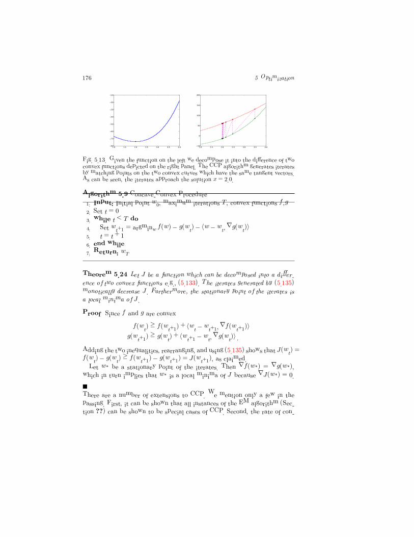
176 5 Optimization
��� ��� ��� ��� ��� ��� �����
��
��
��
��
��
��
��
��� ��� ��� ��� ��� ��� �����
�
��
���
���
���
Fig. 5.13. Given the function on the left we decompose it into the difference of twoconvex functions depicted on the right panel. The CCP algorithm generates iteratesby matching points on the two convex curves which have the same tangent vectors.As can be seen, the iterates approach the solution x = 2.0.
Algorithm 5.9 Concave-Convex Procedure
1: Input: Initial point w0, maximum iterations T , convex functions f ,g
2: Set t = 0
3: while t < T do
4: Set wt+1 = argminw f(w)− g(wt)− �w − wt�∇g(wt)�
5: t = t+ 1
6: end while
7: Return: wT
Theorem 5.24 Let J be a function which can be decomposed into a differ-
ence of two convex functions e.g., (5.133). The iterates generated by (5.135)
monotically decrease J . Furthermore, the stationary point of the iterates is
a local minima of J .
Proof Since f and g are convex
f(wt) ≥ f(wt+1) + �wt − wt+1�∇f(wt+1)�
g(wt+1) ≥ g(wt) + �wt+1 − wt�∇g(wt)� .
Adding the two inequalities, rearranging, and using (5.135) shows that J(wt) =
f(wt)− g(wt) ≥ f(wt+1)− g(wt+1) = J(wt+1), as claimed.
Let w∗ be a stationary point of the iterates. Then ∇f(w∗) = ∇g(w∗),
which in turn implies that w∗ is a local minima of J because ∇J(w∗) = 0.
There are a number of extensions to CCP. We mention only a few in the
passing. First, it can be shown that all instances of the EM algorithm (Sec-
tion ??) can be shown to be special cases of CCP. Second, the rate of con-
5.6 Some Practical Advice 177
vergence of CCP is related to the eigenvalues of the positive semi-definite
matrix ∇2(f + g). Third, CCP can also be extended to solve constrained
problems of the form:
minw
f0(w)− g0(w)
s.t. fi(w)− gi(w) ≤ ci for i = 1� . . . � n.
where, as before, fi and gi for i = 0� 1� . . . � n are assumed convex. At every
iteration, we replace gi by its first order Taylor approximation and solve the
following constrained convex problem:
minw
f0(w)− g0(wt) + �w − wt�∇g0(wt)�
s.t. fi(w)− gi(wt) + �w − wt�∇gi(wt)� ≤ ci for i = 1� . . . � n.
5.6 Some Practical Advice
The range of optimization algorithms we presented in this chapter might be
somewhat intimidating for the beginner. Some simple rules of thumb can
alleviate this anxiety
Code Reuse: Implementing an efficient optimization algorithm correctly
is both time consuming and error prone. Therefore, as far as possible use
existing libraries. A number of high class optimization libraries both com-
mercial and open source exist.
Unconstrained Problems: For unconstrained minimization of a smooth
convex function LBFGS (Section 5.2.6.1 is the algorithm of choice. In many
practical situations the spectral gradient method (Section 5.2.6.2) is also
very competitive. It also has the added advantage of being easy to imple-
ment. If the function to be minimized is non-smooth then Bundle methods
(Section 5.2.7) are to be preferred. Amongst the different formulations, the
Bundle Trust algorithm tends to be quite robust.
Constrained Problems: For constrained problems it is very important
to understand the nature of the constraints. Simple equality (Ax = b) and
box (l ≤ x ≤ u) constraints are easier to handle than general non-linear
constraints. If the objective function is smooth, the constraint set Ω is simple,
and orthogonal projections PΩ are easy to compute, then spectral projected
gradient (Section 5.3.1) is the method of choice. If the optimization problem
is a QP or an LP then specialized solvers tend to be much faster than general
purpose solvers.
178 5 Optimization
Large Scale Problems: If your parameter vector is high dimensional then
consider coordinate descent (Section 5.2.2) especially if the one dimensional
line search along a coordinate can be carried out efficiently. If the objective
function is made up of a summation of large number of terms, consider
stochastic gradient descent (Section 5.4.1). Although both these algorithms
do not guarantee a very accurate solution, practical experience shows that
for large scale machine learning problems this is rarely necessary.
Duality: Sometimes problems which are hard to optimize in the primal
may become simpler in the dual. For instance, if the objective function is
strongly convex but non-smooth, its Fenchel conjugate is smooth with a
Lipschitz continuous gradient.
Problems
Problem 5.1 �Intersection of Convex Sets �1}) If C1 and C2 are con-
vex sets, then show that C1 ∩ C2 is also convex. Extend your result to show
that�n
i=1Ci are convex if Ci are convex.
Problem 5.2 �Linear Transform of Convex Sets �1}) Given a set C ⊂
Rn and a linear transform A ∈ R
m×n, define AC := {y = Ax : x ∈ C}. If
C is convex then show that AC is also convex.
Problem 5.3 �Convex Combinations �1}) Show that a subset of Rn is
convex if and only if it contains all the convex combination of its elements.
Problem 5.4 �Convex Hull �2}) Show that the convex hull, conv(X) is
the smallest convex set which contains X.
Problem 5.5 �Epigraph of a Convex Function �2}) Show that a func-
tion satisfies Definition 5.3 if, and only if, its epigraph is convex.
Problem 5.6 Prove the Jensen’s inequality (5.6).
Problem 5.7 �Strong convexity of the negative entropy �3}) Show that
the negative entropy (5.15) is 1-strongly convex with respect to the �·�1 norm
on the simplex. Hint: First show that φ(t) := (t − 1) log t − 2 (t−1)2
t+1 ≥ 0 for
all t ≥ 0. Next substitute t = xi/yi to show that�
i
(xi − yi) logxiyi≥ �x− y�21 .
5.6 Some Practical Advice 179
Problem 5.8 �Strongly Convex Functions �2}) Prove 5.16, 5.17, 5.18
and 5.19.
Problem 5.9 �Convex Functions with Lipschitz Continuous Gradient �2})
Prove 5.22, 5.23, 5.24 and 5.25.
Problem 5.10 �One Dimensional Projection �1}) If f : Rd → R is
convex, then show that for an arbitrary x and p in Rd the one dimensional
function Φ(η) := f(x+ ηp) is also convex.
Problem 5.11 �Quasi-Convex Functions �2}) In Section 5.1 we showed
that the below-sets of a convex function Xc := {x | f(x) ≤ c} are convex. Give
a counter-example to show that the converse is not true, that is, there exist
non-convex functions whose below-sets are convex. This class of functions is
called Quasi-Convex.
Problem 5.12 �Gradient of the p-norm �1}) Show that the gradient of
the p-norm (5.31) is given by (5.32).
Problem 5.13 Derive the Fenchel conjugate of the following functions
f(x) =
�0 if x ∈ C
∞ otherwise.where C is a convex set
f(x) = ax+ b
f(x) =1
2x�Ax where A is a positive definite matrix
f(x) = − log(x)
f(x) = exp(x)
f(x) = x log(x)
Problem 5.14 �Convergence of gradient descent �2}) Suppose J has
a Lipschitz continuous gradient with modulus L. Then show that Algorithm
5.2 with an inexact line search satisfying the Wolfe conditions (5.42) and
(5.43) will return a solution wt with �∇J(wt)� ≤ � in at most O(1/�2) iter-
ations.
Problem 5.15 Show that
1 +�T
t=11t�T
t=11√t
≤1√T
180 5 Optimization
Problem 5.16 �Coordinate Descent for Quadratic Programming �2})
Derive a projection based method which uses coordinate descent to generate
directions of descent for solving the following box constrained QP:
minw∈�
n
1
2w�Qw + c�w
s.t. l ≤ w ≤ u.
You may assume that Q is positive definite and l and u are scalars.
Problem 5.17 �Dual of a LP �1}) Show that the dual of the LP (5.122)
is (5.115). In other words, we recover the primal by computing the dual of
the dual.